Differential expression between groups using pseudobulk
Sarah Williams
Last updated: 2024-05-28
Checks: 7 0
Knit directory: spatialsnippets/
This reproducible R Markdown analysis was created with workflowr (version 1.7.1). The Checks tab describes the reproducibility checks that were applied when the results were created. The Past versions tab lists the development history.
Great! Since the R Markdown file has been committed to the Git repository, you know the exact version of the code that produced these results.
Great job! The global environment was empty. Objects defined in the global environment can affect the analysis in your R Markdown file in unknown ways. For reproduciblity it’s best to always run the code in an empty environment.
The command set.seed(20231017) was run prior to running
the code in the R Markdown file. Setting a seed ensures that any results
that rely on randomness, e.g. subsampling or permutations, are
reproducible.
Great job! Recording the operating system, R version, and package versions is critical for reproducibility.
Nice! There were no cached chunks for this analysis, so you can be confident that you successfully produced the results during this run.
Great job! Using relative paths to the files within your workflowr project makes it easier to run your code on other machines.
Great! You are using Git for version control. Tracking code development and connecting the code version to the results is critical for reproducibility.
The results in this page were generated with repository version dd0f089. See the Past versions tab to see a history of the changes made to the R Markdown and HTML files.
Note that you need to be careful to ensure that all relevant files for
the analysis have been committed to Git prior to generating the results
(you can use wflow_publish or
wflow_git_commit). workflowr only checks the R Markdown
file, but you know if there are other scripts or data files that it
depends on. Below is the status of the Git repository when the results
were generated:
Ignored files:
    Ignored:    .Rhistory
    Ignored:    .Rproj.user/
    Ignored:    renv/library/
    Ignored:    renv/staging/
Note that any generated files, e.g. HTML, png, CSS, etc., are not included in this status report because it is ok for generated content to have uncommitted changes.
These are the previous versions of the repository in which changes were
made to the R Markdown (analysis/e_DEPseudobulk_insitu.Rmd)
and HTML (docs/e_DEPseudobulk_insitu.html) files. If you’ve
configured a remote Git repository (see ?wflow_git_remote),
click on the hyperlinks in the table below to view the files as they
were in that past version.
| File | Version | Author | Date | Message |
|---|---|---|---|---|
| Rmd | dd0f089 | swbioinf | 2024-05-28 | wflow_publish("analysis/e_DEPseudobulk_insitu.Rmd") |
| html | d6d841a | swbioinf | 2024-05-22 | Build site. |
| Rmd | 9c53965 | swbioinf | 2024-05-22 | wflow_publish("analysis/e_DEPseudobulk_insitu.Rmd") |
| html | 58ee2ec | swbioinf | 2024-05-22 | Build site. |
| Rmd | 36dd228 | swbioinf | 2024-05-22 | wflow_publish("analysis/e_DEPseudobulk_insitu.Rmd") |
| html | 5a9d7e9 | swbioinf | 2024-05-16 | Build site. |
| Rmd | c67ef86 | swbioinf | 2024-05-16 | wflow_publish("analysis/e_DEPseudobulk_insitu.Rmd") |
| html | c77f76c | swbioinf | 2024-05-07 | Build site. |
| Rmd | 7b0be93 | swbioinf | 2024-05-07 | wflow_publish(c("analysis/index.Rmd", "analysis/e_DEPseudobulk_insitu.Rmd", |
Overview
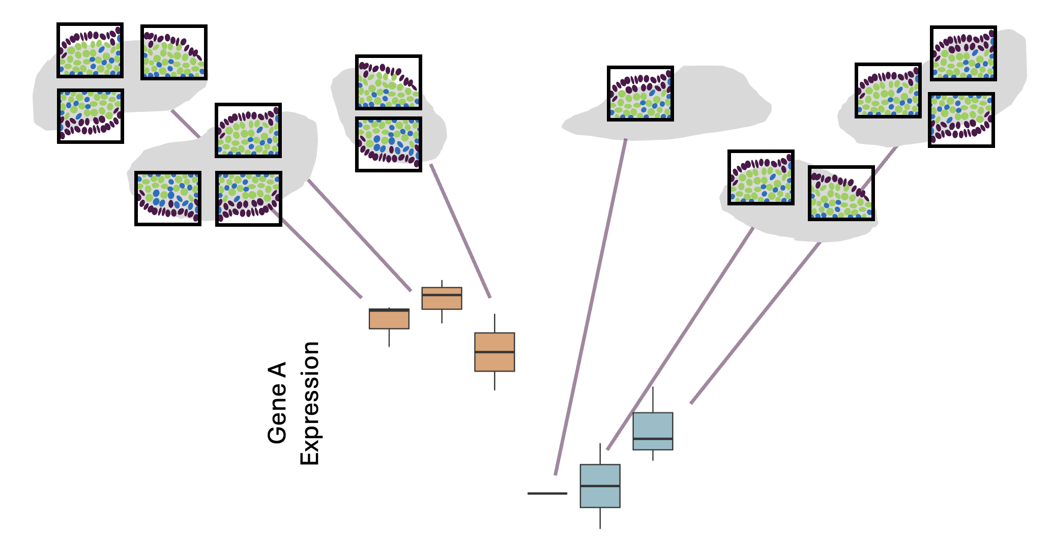
Once we have identified cell types present in the samples, its typical to test how gene expression changes between experimental conditions, within each different cell type. Some cell types may be dramatically affected by the experimental conditions, while others are not. Likewise some genes may change only in a specific cell type, whereas others show a more general difference.
This document describes how to apply a pseudobulk approach to test for differences between groups, accounting for biological replicates. This is very similar to how a non-spatial single cell experiment may be analysed.
In a pseudobulk approach counts are obtaing by pooling together groups of cells; in this case cells from the of the same type from the same fov. These pooled counts can then be analysed more like a bulk RNAseq experiment.
Note that there are other approaches to calculate differential expression in this kind of data - including those that make use of individual cells.
This requires:
- Biological replicates for each group
- Assigned cell types
- [Optionally] Multiple fovs measured per sample
For example:
- What genes are differentially expressed in epithelial cells in Crohn’s disease vs healthy individuals?
- How do genes change with treatment in each different cell type in my sample?
Steps:
- Calculate pseudobulk
- Filter to testable pseudobulk groups (enough cells to pool)
- Filter to testable genes (enough expression to see changes)
- Test for changes in gene expression
- Plot DE results and individual genes.
Worked example
How does gene expression change within each cell type between Ulcerative colitis or Crohn’s disease, and Healthy controls?
Load libraries and data
library(Seurat)
library(speckle)
library(tidyverse)
library(limma)
library(DT)
library(edgeR)
data_dir <- file.path("~/projects/spatialsnippets/datasets/GSE234713_IBDcosmx_GarridoTrigo2023/processed_data")
seurat_file_01_loaded <- file.path(data_dir, "GSE234713_CosMx_IBD_seurat_01_loaded.RDS")so <- readRDS(seurat_file_01_loaded)Experimental design
There are three individuals per condition (one tissue sample from each individual). With multiple fovs on each physical tissue sample.
sample_table <- select(as_tibble(so@meta.data), condition, individual_code, fov_name) %>%
  unique() %>%
  group_by(condition, individual_code) %>%
  summarise(n_fovs= n(), item = str_c(fov_name, collapse = ", "))

DT::datatable(sample_table)
Count how many cells of each type in your data
Using a pseudobulk approach.
- Need at least x reads in a cell to include it
- Need at least x cells of a celltype within an fov to include that
- Can only test where we have at least 2 samples on each side of a contrast.
min_reads_per_cell <- 200

ggplot(so@meta.data, aes(x=nCount_RNA)) +
  geom_density() +
  geom_vline(xintercept = min_reads_per_cell, lty=3) +
  scale_x_log10() +
  theme_bw()+
  ggtitle("How many reads per cell?")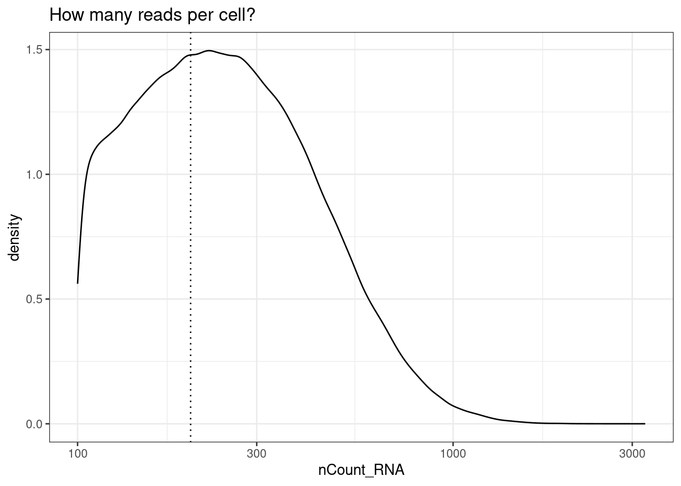
| Version | Author | Date |
|---|---|---|
| c77f76c | swbioinf | 2024-05-07 |
so<- so[,so$nCount_RNA >= min_reads_per_cell]We will pool each celltype within each fov (cluster_group). But there needs to be a certain number of cells for that to work - less than a certain number of cells and a pseudobulk pool will be excluded.
Note there are much fewer t-cells overall, but given that we have a high number of samples, there should still be enough to include. Its typical that some of the less common cell types are difficult or impossible to reliably test.
min_cells_per_fovcluster <- 20

so$fov_cluster <- paste0(so$fov_name,"_", so$celltype_subset)

celltype_summary_table <- so@meta.data %>%
  group_by(condition, group, individual_code, fov_name, celltype_subset, fov_cluster) %>%
  summarise(cells=n(), .groups = 'drop')
DT::datatable(celltype_summary_table)
ggplot(celltype_summary_table, aes(x=cells, col=celltype_subset)) +
geom_density() +
geom_vline(xintercept=min_cells_per_fovcluster, lty=3) +
geom_rug() +
scale_x_log10() +
theme_bw() +
ggtitle("How many cells per fov-cluster?")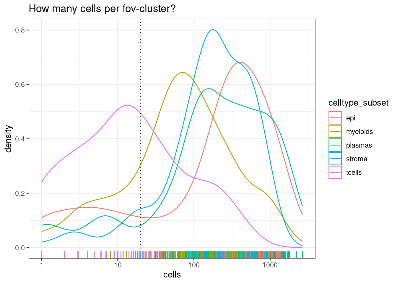
| Version | Author | Date |
|---|---|---|
| c77f76c | swbioinf | 2024-05-07 |
passed_fov_clusters <- celltype_summary_table$fov_cluster[celltype_summary_table$cells >= min_cells_per_fovcluster]Calculate pseudobulk
pseudobulk_counts <- PseudobulkExpression(so, assays = "RNA", layer="counts",  method = 'aggregate', group.by = 'fov_cluster')
pseudobulk_counts_matrix <- pseudobulk_counts[["RNA"]]

# CHange - back to _. Ideally we'd have neither, but - will cause problems later
colnames(pseudobulk_counts_matrix)<-gsub("-","_",colnames(pseudobulk_counts_matrix))
Keep only the passed fovs
pseudobulk_counts_matrix <- pseudobulk_counts_matrix[,passed_fov_clusters]

# pull in relevant annotation in a matched order
pseudobulk_anno_table <- celltype_summary_table
match_order <- match(passed_fov_clusters, pseudobulk_anno_table$fov_cluster)
pseudobulk_anno_table <- pseudobulk_anno_table[match_order,]
stopifnot(all(colnames(pseudobulk_counts_matrix) == pseudobulk_anno_table$fov_cluster  ))
Calculate Differential Expression
min_samples_to_calc <- 2 # require 2 samples on on either side of contrast

de_result_list <- list()

# celltype_subset is a matrix
for (the_celltype in levels(so$celltype_subset)) {

  anno_table.this   <- pseudobulk_anno_table[pseudobulk_anno_table$celltype_subset == the_celltype,]
  count_matrix.this <- pseudobulk_counts_matrix[,anno_table.this$fov_cluster]

  print(the_celltype)

  # skip clusters with nothing
  if( nrow(anno_table.this) < 1 ) {next}

  # Setup objects for limma
  dge <- DGEList(count_matrix.this)
  dge <- calcNormFactors(dge)

  # Build model
  group           <- anno_table.this$group
  individual_code <- anno_table.this$individual_code

  # To do any calculations, we need at least 2 pseudobulk groups per contrast.
  # there are plenty in this experiemnt, but with less replicates and rare cell types
  # it may be neccesary to check and skip certain contrasts

  # Model design
  design    <- model.matrix( ~0 + group)

  vm  <- voom(dge, design = design, plot = FALSE)

  # Adding dupliate correlation to use individual fovs, rather than pooled per biosample
  corrfit <- duplicateCorrelation(vm, design, block=individual_code)
  fit     <- lmFit(vm, design, correlation = corrfit$consensus, block=individual_code)

  # Then fit contrasts and run ebayes
  contrasts <- makeContrasts(UCvHC  = groupUC - groupHC,
                             CDvHC  = groupCD - groupHC,
                           levels=coef(fit))

  fit <- contrasts.fit(fit, contrasts)
  fit <- eBayes(fit)


  for ( the_coef in colnames(contrasts) ) {
    de_result.this <- topTable(fit, n = Inf, adjust.method = "BH", coef = the_coef) %>%
      rownames_to_column("target") %>%
      mutate(contrast=the_coef,
             celltype=the_celltype) %>%
      select(celltype,contrast,target,everything()) %>%
      arrange(P.Value)


      de_result_list[[paste(the_celltype, the_coef, sep="_")]] <- de_result.this

  }


}
[1] "epi"
[1] "myeloids"
[1] "plasmas"
[1] "stroma"
[1] "tcells"de_results_all <- bind_rows(de_result_list)
de_results_sig <- filter(de_results_all, adj.P.Val < 0.01)Table of significant results.
DT::datatable(de_results_sig)DE plots
library(ggrepel) # gg_repel, For non-overlapping gene labels
make_ma_style_plot <- function(res_table, pval_threshold = 0.01, n_genes_to_label = 10) {
p <- ggplot(res_table, aes(x=AveExpr, y=logFC, col=adj.P.Val < pval_threshold) ) +
geom_hline(yintercept = c(0), col='grey80') +
geom_point(pch=3) +
geom_text_repel(data = head(arrange(filter(res_table , adj.P.Val < pval_threshold ), P.Value), n=5),
mapping = aes(label=target), col="red" ) +
theme_bw() +
geom_hline(yintercept = c(-1,1), lty=3) +
scale_colour_manual(values = c('FALSE'="black", 'TRUE'="red")) +
theme(legend.position = 'none')
return(p)
}#res_table.UCvHC.epi <- filter(de_results_all, contrast == "UCvHC", celltype=="epi")
make_ma_style_plot(res_table = filter(de_results_all, contrast == "UCvHC", celltype=="epi"))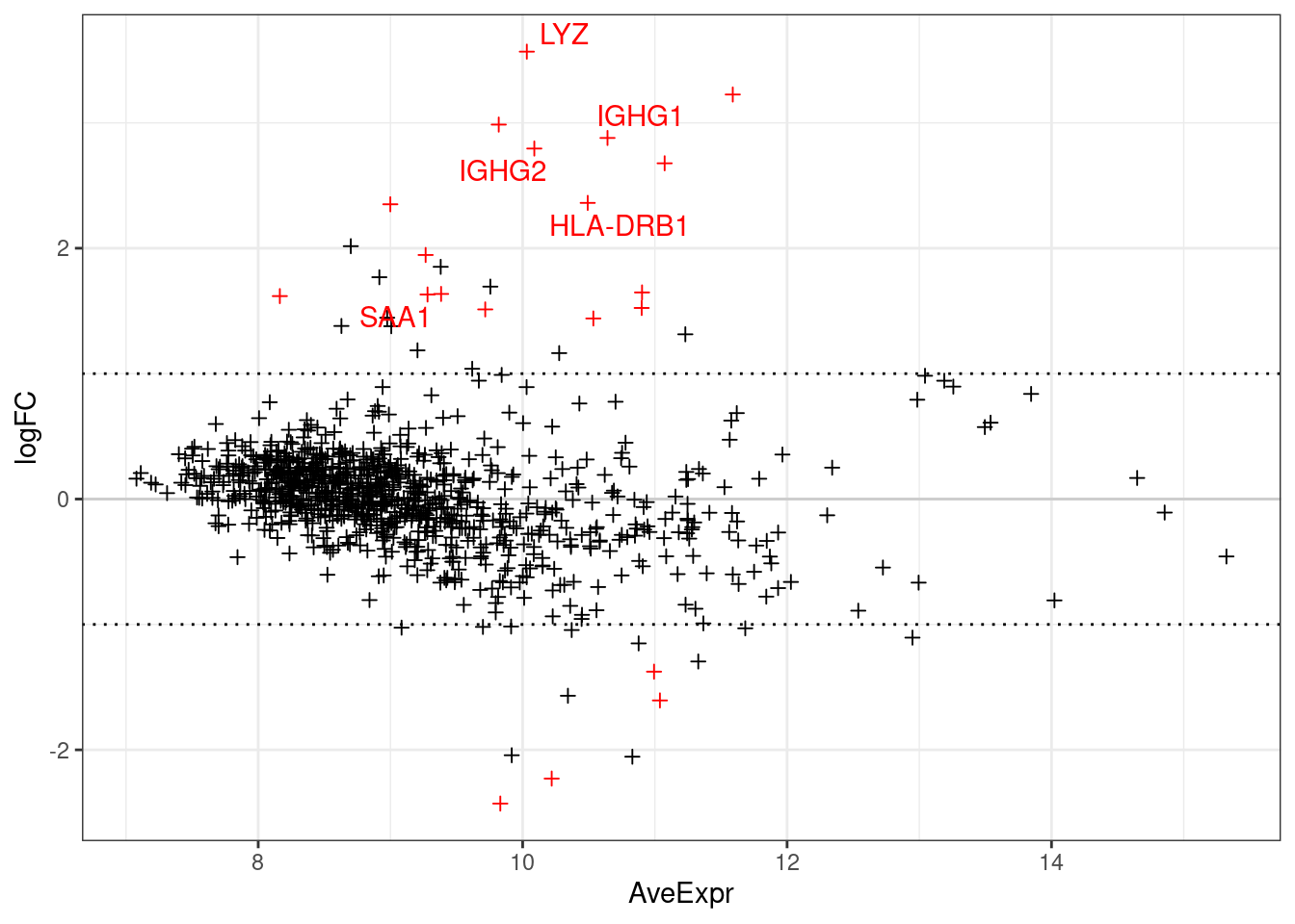
| Version | Author | Date |
|---|---|---|
| 5a9d7e9 | swbioinf | 2024-05-16 |
make_ma_style_plot(res_table = filter(de_results_all, contrast == "UCvHC", celltype=="tcells"))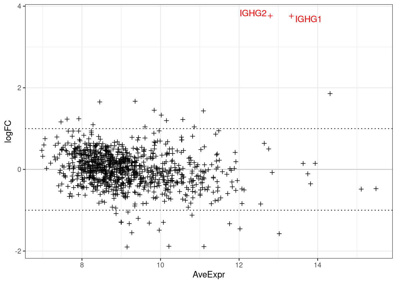
| Version | Author | Date |
|---|---|---|
| 5a9d7e9 | swbioinf | 2024-05-16 |
make_ma_style_plot(res_table = filter(de_results_all, contrast == "UCvHC", celltype=="stroma"))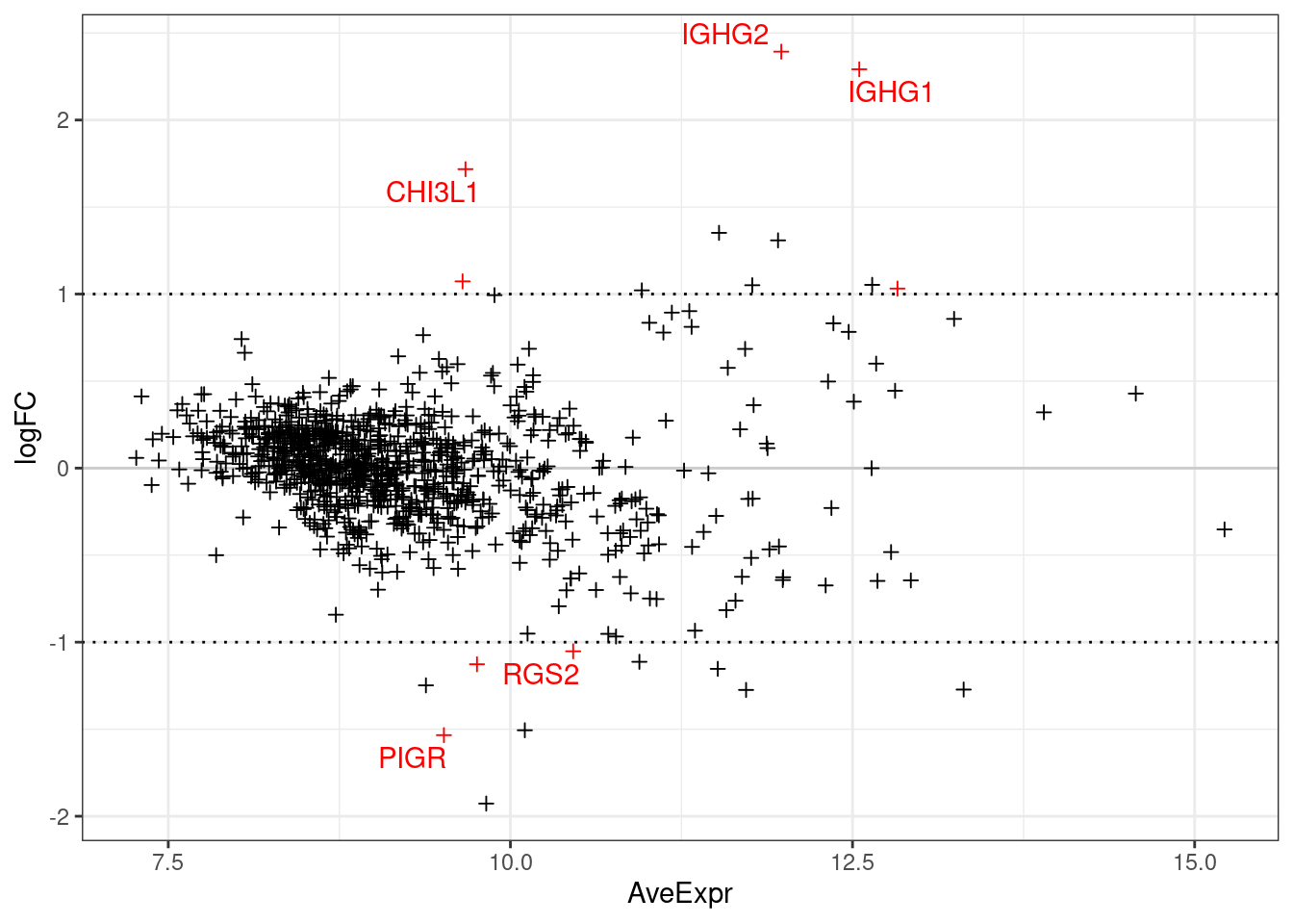
| Version | Author | Date |
|---|---|---|
| 5a9d7e9 | swbioinf | 2024-05-16 |
Check some examples
Its always worth visualising how the expression of your differentially expressed genes really looks, with respect to your experimental design. How best to do this depends on your experiment.
The results suggests that TNFRSF18 was significantly DE between individuals with Ulcerative Colitis and Healthy Controls in plasma cells. There’s some very convenient seurat plots below;
VlnPlot(subset(so, celltype_subset == "plasmas"), features = "TNFRSF18", group.by = 'group', alpha = 0.1)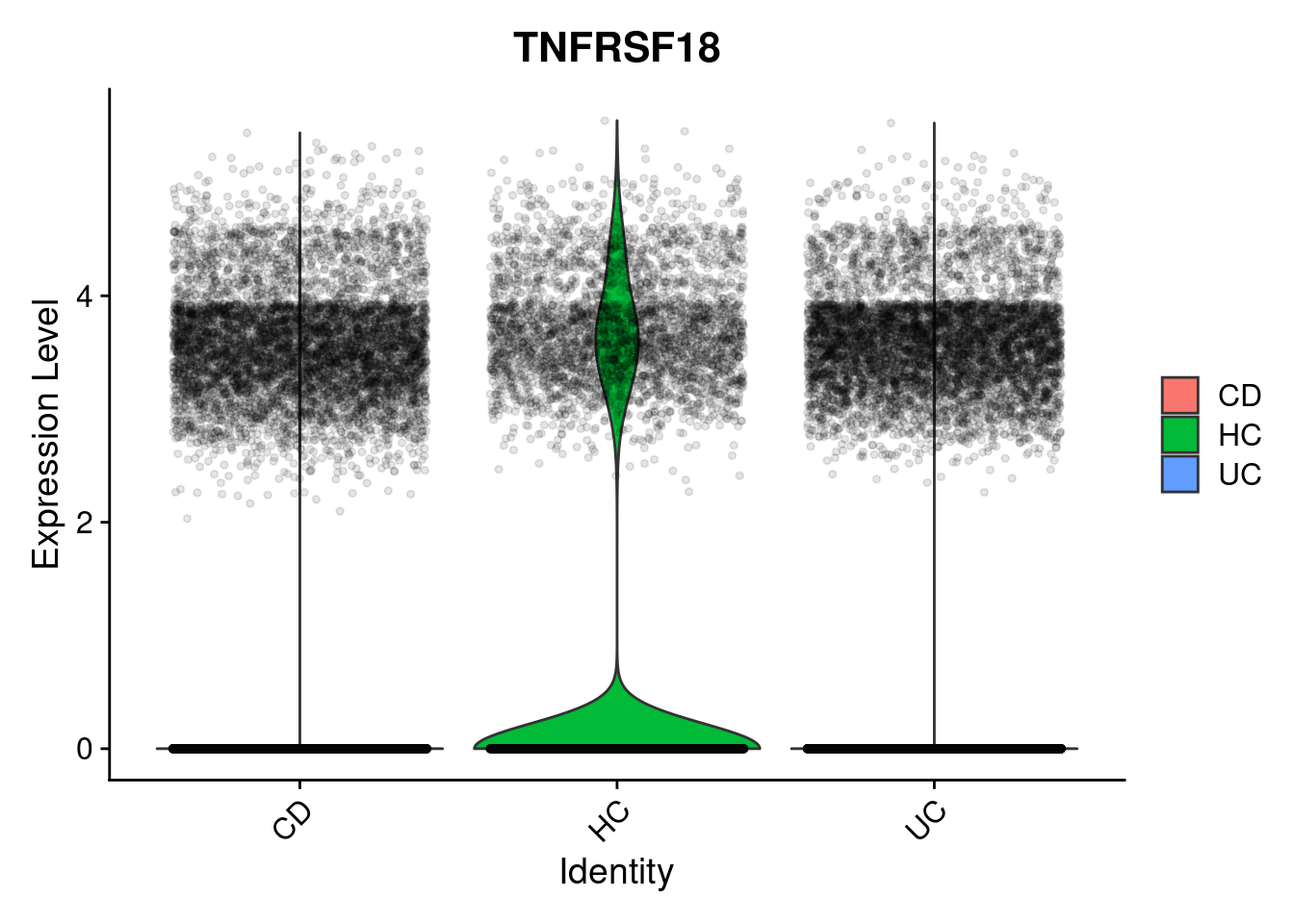
| Version | Author | Date |
|---|---|---|
| 5a9d7e9 | swbioinf | 2024-05-16 |
FeaturePlot(so, "TNFRSF18", split.by = "group")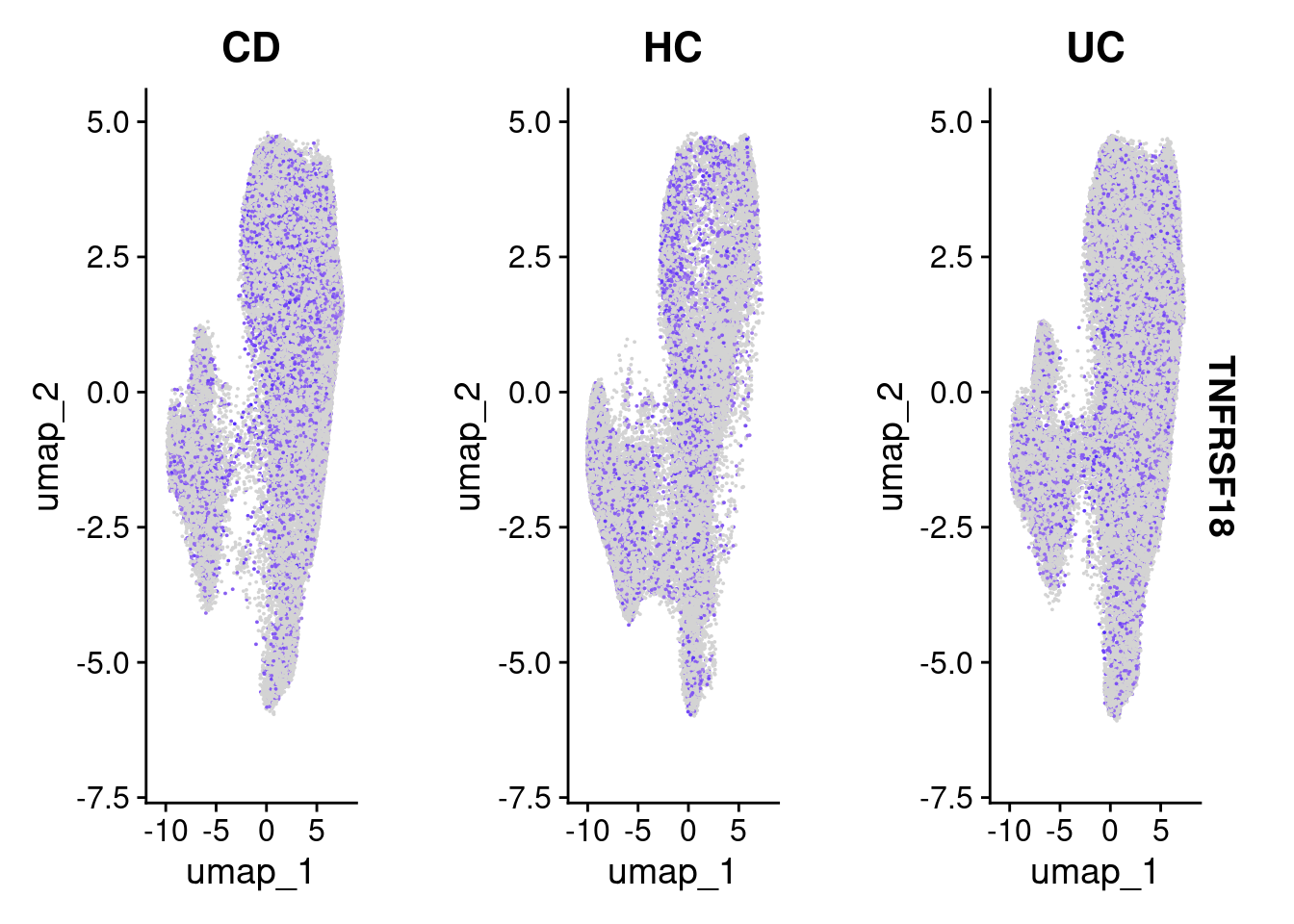
| Version | Author | Date |
|---|---|---|
| 5a9d7e9 | swbioinf | 2024-05-16 |
But it gets difficult to summarise data at the single cell level. We can also use the the normalised pseudobulk expression to see how gene expression varies within each fov,individual,celltype and condition - The plot below shows an overview of TNFRSF18 across the entire experiment.
NB: We have to plot normalised expression instead of the raw counts as there are vastly different numbers of cells in each fov+celltype grouping.
# Get tmm normalised coutns for all pseudobulk
# WHen we did the DE we calculated this a celltype at a time, so values might differ slightly!
dge <- DGEList(pseudobulk_counts_matrix)
dge <- calcNormFactors(dge)
norm_pseudobulk <- cpm(dge , log=TRUE) # uses tmm normalisation
# Plot expression for TNFRSF18
plottable <- cbind(pseudobulk_anno_table, expression = norm_pseudobulk["TNFRSF18",])
ggplot(plottable, aes(x=individual_code, y=expression, col=condition )) +
geom_boxplot(outlier.shape = NA) +
geom_point() +
theme_bw() +
theme(axis.text.x=element_text(angle = -90, hjust = 0)) +
facet_wrap(~celltype_subset) 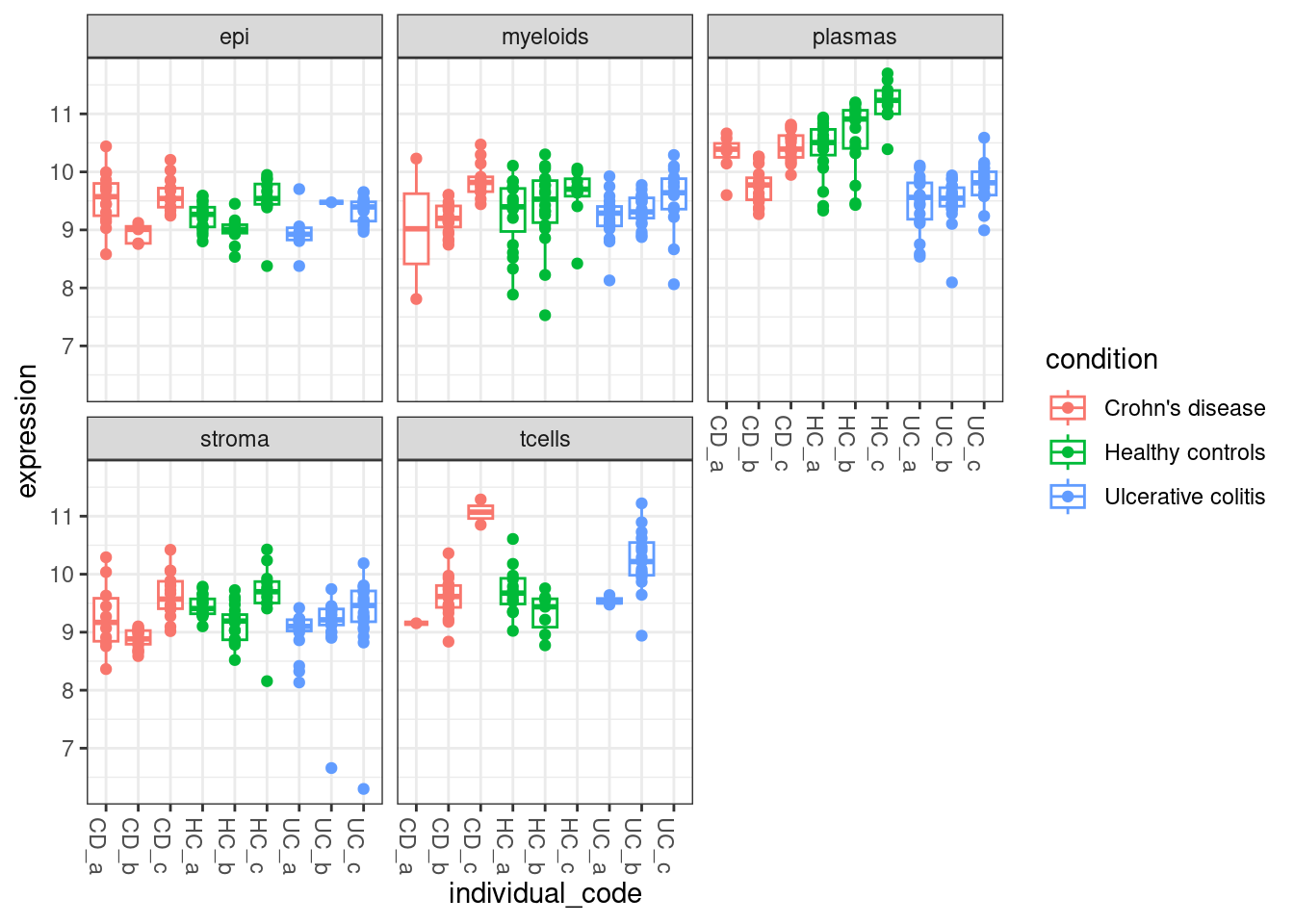
| Version | Author | Date |
|---|---|---|
| 5a9d7e9 | swbioinf | 2024-05-16 |
And you can compare that with IGHG1, which was flagged at differentially expressed across multiple cell types.
plottable <- cbind(pseudobulk_anno_table, expression = norm_pseudobulk["IGHG1",])
ggplot(plottable, aes(x=individual_code, y=expression, col=condition )) +
geom_boxplot(outlier.shape = NA) +
geom_point() +
theme_bw() +
theme(axis.text.x=element_text(angle = -90, hjust = 0)) +
facet_wrap(~celltype_subset) 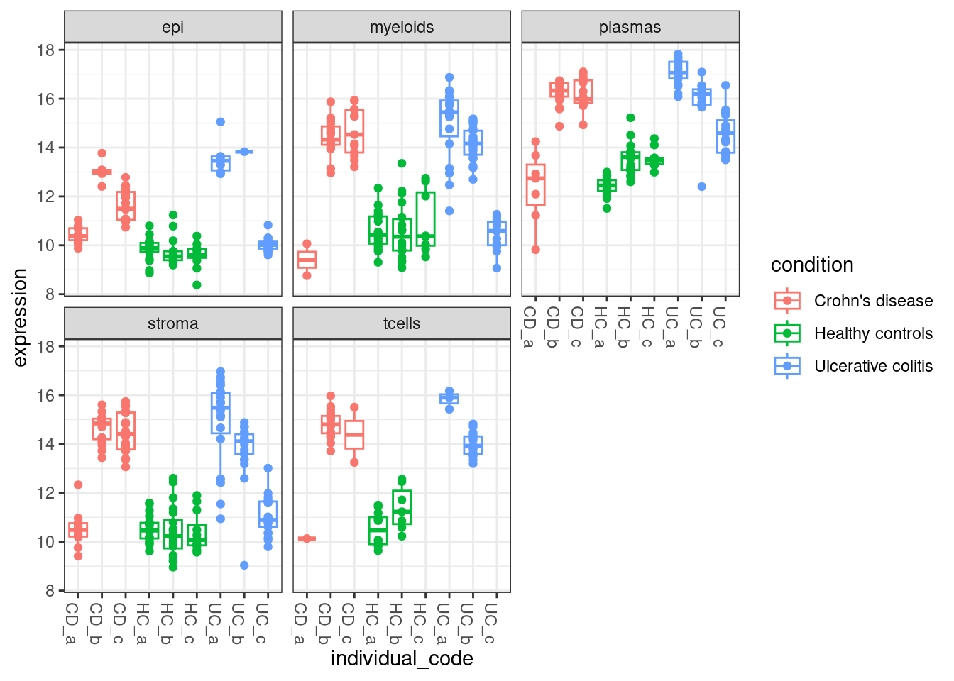
| Version | Author | Date |
|---|---|---|
| 5a9d7e9 | swbioinf | 2024-05-16 |
Code Snippet
library(Seurat)
library(edgeR)
library(limma)
min_reads_per_cell <- 200
min_cells_per_fovcluster <- 20
min_samples_to_calc <- 2 # require 2 samples on on either side of contrast
# Remove cells with too few counts
so <- so[,so$nCount_RNA >= min_reads_per_cell]
# Define fov+cluster groups, with all relevant sample annotation
# remove those with too few cells.
so$fov_cluster <- paste0(so$fov_name,"_", so$celltype_subset)
celltype_summary_table <- so@meta.data %>%
group_by(condition, group, individual_code, fov_name, celltype_subset, fov_cluster) %>%
summarise(cells=n(), .groups = 'drop')
# Calculate pseudobulk for each fov+cluster group
pseudobulk_counts <- PseudobulkExpression(so, assays = "RNA", layer="counts", method = 'aggregate', group.by = 'fov_cluster')
pseudobulk_counts_matrix <- pseudobulk_counts[["RNA"]]
# Change - back to _. Ideally have neither and skip this step
colnames(pseudobulk_counts_matrix)<-gsub("-","_",colnames(pseudobulk_counts_matrix))
# Determin fov_clusters with eough cells
# Filter both pseudobulk matrix and pseudobulk annotation
passed_fov_clusters <- celltype_summary_table$fov_cluster[celltype_summary_table$cells >= min_cells_per_fovcluster]
pseudobulk_counts_matrix <- pseudobulk_counts_matrix[,passed_fov_clusters]
pseudobulk_anno_table <- celltype_summary_table[passed_fov_clusters,]
# Calculate DE across every celltype
de_result_list <- list()
for (the_celltype in levels(so$celltype_subset)) {
anno_table.this <- pseudobulk_anno_table[pseudobulk_anno_table$celltype_subset == the_celltype,]
count_matrix.this <- pseudobulk_counts_matrix[,anno_table.this$fov_cluster]
print(the_celltype)
# skip clusters with nothing
if( nrow(anno_table.this) < 1 ) {next}
# Setup objects for limma
dge <- DGEList(count_matrix.this)
dge <- calcNormFactors(dge)
# Build model
group <- anno_table.this$group
individual_code <- anno_table.this$individual_code
# To do any calculations, we need at least 2 pseudobulk groups per contrast.
# there are plenty in this experiemnt, but with less replicates and rare cell types
# it may be neccesary to check and skip certain contrasts
# Model design
design <- model.matrix( ~0 + group)
vm <- voom(dge, design = design, plot = FALSE)
# Adding dupliate correlation to use individual fovs, rather than pooled per biosample
corrfit <- duplicateCorrelation(vm, design, block=individual_code)
fit <- lmFit(vm, design, correlation = corrfit$consensus, block=individual_code)
# Then fit contrasts and run ebayes
contrasts <- makeContrasts(UCvHC = groupUC - groupHC
levels=coef(fit))
fit <- contrasts.fit(fit, contrasts)
fit <- eBayes(fit)
for ( the_coef in colnames(contrasts) ) {
de_result.this <- topTable(fit, n = Inf, adjust.method = "BH", coef = the_coef) %>%
rownames_to_column("target") %>%
mutate(contrast=the_coef,
celltype=the_celltype) %>%
select(celltype,contrast,target,everything()) %>%
arrange(P.Value)
de_result_list[[paste(the_celltype, the_coef, sep="_")]] <- de_result.this
}
}
de_results_all <- bind_rows(de_result_list)
de_results_sig <- filter(de_results_all, adj.P.Val < 0.01)Results
DT::datatable(head(de_results_all))This table is the typical output of limma tests; With a couple of extra columns added by our code.
- celltype: The celltype being tested (Added by example code)
- contrast: The contrast being tested (Added by example code)
- target : The gene name (Added by example code, is the rowname in limma output)
- rownames : The tested cell types
- logFC : Log 2 fold change between tested groups.
For a test of Test-Con;
- At logFC +1, A is doubled B.
- At logFC -1, A is half of B.
- A logFC 0 indicates no change.
- AveExpr : Average expression of a gene across all replicates.
- t : Moderated T-statistic. See Limma documentation.
- P.Value : P.value
- adj.P.Val : A multiple-hypothesis corrected p-value
- B : B statistic (rarely used). See Limma documentation.
More Information
Todo
sessionInfo()R version 4.3.2 (2023-10-31)
Platform: x86_64-pc-linux-gnu (64-bit)
Running under: Ubuntu 22.04.4 LTS
Matrix products: default
BLAS: /usr/lib/x86_64-linux-gnu/openblas-pthread/libblas.so.3
LAPACK: /usr/lib/x86_64-linux-gnu/openblas-pthread/libopenblasp-r0.3.20.so; LAPACK version 3.10.0
locale:
[1] LC_CTYPE=en_AU.UTF-8 LC_NUMERIC=C
[3] LC_TIME=en_AU.UTF-8 LC_COLLATE=en_AU.UTF-8
[5] LC_MONETARY=en_AU.UTF-8 LC_MESSAGES=en_AU.UTF-8
[7] LC_PAPER=en_AU.UTF-8 LC_NAME=C
[9] LC_ADDRESS=C LC_TELEPHONE=C
[11] LC_MEASUREMENT=en_AU.UTF-8 LC_IDENTIFICATION=C
time zone: Etc/UTC
tzcode source: system (glibc)
attached base packages:
[1] stats graphics grDevices datasets utils methods base
other attached packages:
[1] ggrepel_0.9.5 edgeR_4.0.16 DT_0.33 limma_3.58.1
[5] lubridate_1.9.3 forcats_1.0.0 stringr_1.5.1 dplyr_1.1.4
[9] purrr_1.0.2 readr_2.1.5 tidyr_1.3.1 tibble_3.2.1
[13] ggplot2_3.5.0 tidyverse_2.0.0 speckle_1.2.0 Seurat_5.0.3
[17] SeuratObject_5.0.1 sp_2.1-3 workflowr_1.7.1
loaded via a namespace (and not attached):
[1] RcppAnnoy_0.0.22 splines_4.3.2
[3] later_1.3.2 bitops_1.0-7
[5] polyclip_1.10-6 fastDummies_1.7.3
[7] lifecycle_1.0.4 rprojroot_2.0.4
[9] globals_0.16.3 processx_3.8.4
[11] lattice_0.22-6 MASS_7.3-60.0.1
[13] crosstalk_1.2.1 magrittr_2.0.3
[15] plotly_4.10.4 sass_0.4.9
[17] rmarkdown_2.26 jquerylib_0.1.4
[19] yaml_2.3.8 httpuv_1.6.15
[21] sctransform_0.4.1 spam_2.10-0
[23] spatstat.sparse_3.0-3 reticulate_1.35.0
[25] cowplot_1.1.3 pbapply_1.7-2
[27] RColorBrewer_1.1-3 abind_1.4-5
[29] zlibbioc_1.48.2 Rtsne_0.17
[31] GenomicRanges_1.54.1 BiocGenerics_0.48.1
[33] RCurl_1.98-1.14 git2r_0.33.0
[35] GenomeInfoDbData_1.2.11 IRanges_2.36.0
[37] S4Vectors_0.40.2 irlba_2.3.5.1
[39] listenv_0.9.1 spatstat.utils_3.0-4
[41] goftest_1.2-3 RSpectra_0.16-1
[43] spatstat.random_3.2-3 fitdistrplus_1.1-11
[45] parallelly_1.37.1 leiden_0.4.3.1
[47] codetools_0.2-20 DelayedArray_0.28.0
[49] tidyselect_1.2.1 farver_2.1.1
[51] matrixStats_1.2.0 stats4_4.3.2
[53] spatstat.explore_3.2-7 jsonlite_1.8.8
[55] progressr_0.14.0 ggridges_0.5.6
[57] survival_3.5-8 tools_4.3.2
[59] ica_1.0-3 Rcpp_1.0.12
[61] glue_1.7.0 gridExtra_2.3
[63] SparseArray_1.2.4 xfun_0.43
[65] MatrixGenerics_1.14.0 GenomeInfoDb_1.38.8
[67] withr_3.0.0 BiocManager_1.30.22
[69] fastmap_1.1.1 fansi_1.0.6
[71] callr_3.7.6 digest_0.6.35
[73] timechange_0.3.0 R6_2.5.1
[75] mime_0.12 colorspace_2.1-0
[77] scattermore_1.2 tensor_1.5
[79] spatstat.data_3.0-4 utf8_1.2.4
[81] generics_0.1.3 renv_1.0.5
[83] data.table_1.15.4 httr_1.4.7
[85] htmlwidgets_1.6.4 S4Arrays_1.2.1
[87] whisker_0.4.1 uwot_0.1.16
[89] pkgconfig_2.0.3 gtable_0.3.4
[91] lmtest_0.9-40 SingleCellExperiment_1.24.0
[93] XVector_0.42.0 htmltools_0.5.8
[95] dotCall64_1.1-1 scales_1.3.0
[97] Biobase_2.62.0 png_0.1-8
[99] knitr_1.45 rstudioapi_0.16.0
[101] tzdb_0.4.0 reshape2_1.4.4
[103] nlme_3.1-164 cachem_1.0.8
[105] zoo_1.8-12 KernSmooth_2.23-22
[107] parallel_4.3.2 miniUI_0.1.1.1
[109] pillar_1.9.0 grid_4.3.2
[111] vctrs_0.6.5 RANN_2.6.1
[113] promises_1.2.1 xtable_1.8-4
[115] cluster_2.1.6 evaluate_0.23
[117] cli_3.6.2 locfit_1.5-9.9
[119] compiler_4.3.2 rlang_1.1.3
[121] crayon_1.5.2 future.apply_1.11.2
[123] labeling_0.4.3 ps_1.7.6
[125] getPass_0.2-4 plyr_1.8.9
[127] fs_1.6.3 stringi_1.8.3
[129] viridisLite_0.4.2 deldir_2.0-4
[131] munsell_0.5.1 lazyeval_0.2.2
[133] spatstat.geom_3.2-9 Matrix_1.6-5
[135] RcppHNSW_0.6.0 hms_1.1.3
[137] patchwork_1.2.0 future_1.33.2
[139] statmod_1.5.0 shiny_1.8.1.1
[141] highr_0.10 SummarizedExperiment_1.32.0
[143] ROCR_1.0-11 igraph_2.0.3
[145] bslib_0.7.0