Analysis
Tina Lasisi
March 13, 2022
Last updated: 2022-03-13
Checks: 6 1
Knit directory: HairManikin_manuscript/
This reproducible R Markdown analysis was created with workflowr (version 1.6.2). The Checks tab describes the reproducibility checks that were applied when the results were created. The Past versions tab lists the development history.
The R Markdown file has unstaged changes. To know which version of the R Markdown file created these results, you’ll want to first commit it to the Git repo. If you’re still working on the analysis, you can ignore this warning. When you’re finished, you can run wflow_publish to commit the R Markdown file and build the HTML.
Great job! The global environment was empty. Objects defined in the global environment can affect the analysis in your R Markdown file in unknown ways. For reproduciblity it’s best to always run the code in an empty environment.
The command set.seed(20211024) was run prior to running the code in the R Markdown file. Setting a seed ensures that any results that rely on randomness, e.g. subsampling or permutations, are reproducible.
Great job! Recording the operating system, R version, and package versions is critical for reproducibility.
Nice! There were no cached chunks for this analysis, so you can be confident that you successfully produced the results during this run.
Great job! Using relative paths to the files within your workflowr project makes it easier to run your code on other machines.
Great! You are using Git for version control. Tracking code development and connecting the code version to the results is critical for reproducibility.
The results in this page were generated with repository version 210cee3. See the Past versions tab to see a history of the changes made to the R Markdown and HTML files.
Note that you need to be careful to ensure that all relevant files for the analysis have been committed to Git prior to generating the results (you can use wflow_publish or wflow_git_commit). workflowr only checks the R Markdown file, but you know if there are other scripts or data files that it depends on. Below is the status of the Git repository when the results were generated:
Ignored files:
    Ignored:    .DS_Store
    Ignored:    .RData
    Ignored:    .Rhistory
    Ignored:    .Rproj.user/
    Ignored:    data/.DS_Store
    Ignored:    data/.Rhistory
    Ignored:    data/current/.DS_Store
    Ignored:    data/raw_manikin_output/.DS_Store

Untracked files:
    Untracked:  data/df_influx.csv
    Untracked:  data/df_long_wetdry_final.csv
    Untracked:  data/df_sum_wetdry.csv
    Untracked:  data/df_wetdry_final.csv
    Untracked:  data/sum_manikin_df.csv

Unstaged changes:
    Modified:   analysis/analysis.Rmd
    Deleted:    data/raw_manikin_output/~$2020_Dec_GH_WigData_reworked.xlsx
Note that any generated files, e.g. HTML, png, CSS, etc., are not included in this status report because it is ok for generated content to have uncommitted changes.
These are the previous versions of the repository in which changes were made to the R Markdown (analysis/analysis.Rmd) and HTML (docs/analysis.html) files. If you’ve configured a remote Git repository (see ?wflow_git_remote), click on the hyperlinks in the table below to view the files as they were in that past version.
| File | Version | Author | Date | Message |
|---|---|---|---|---|
| Rmd | 210cee3 | Tina Lasisi | 2022-03-10 | updated figure size |
| html | 210cee3 | Tina Lasisi | 2022-03-10 | updated figure size |
| Rmd | bf62a07 | Tina Lasisi | 2022-03-10 | Updating analyses + figures |
| html | bf62a07 | Tina Lasisi | 2022-03-10 | Updating analyses + figures |
| html | 1a1f7bc | Tina Lasisi | 2022-03-07 | Build site. |
| Rmd | 7478e4c | Tina Lasisi | 2022-03-07 | updating analyses with models |
| html | c0ce5d2 | Tina Lasisi | 2022-03-06 | Build site. |
| Rmd | 4041aec | Tina Lasisi | 2022-03-06 | wflow_publish(files = "analysis/*", all = TRUE, republish = TRUE, |
| html | 4041aec | Tina Lasisi | 2022-03-06 | wflow_publish(files = "analysis/*", all = TRUE, republish = TRUE, |
| Rmd | a796ceb | Ginawsy | 2022-02-21 | updated sum_manikin_df variable |
| Rmd | 520dcfc | GitHub | 2022-02-16 | Update analysis.Rmd |
| Rmd | 9c5b0d8 | Tina Lasisi | 2022-02-15 | Update analysis + figures |
| html | 9c5b0d8 | Tina Lasisi | 2022-02-15 | Update analysis + figures |
| Rmd | e9fa430 | GitHub | 2022-01-30 | Update analysis.Rmd |
| html | bb36720 | Tina Lasisi | 2022-01-19 | Build site. |
| Rmd | 05389ae | Tina Lasisi | 2022-01-19 | Added figures + analysis placeholders |
| html | 05389ae | Tina Lasisi | 2022-01-19 | Added figures + analysis placeholders |
| Rmd | bb99f1d | Tina Lasisi | 2022-01-08 | Update analysis.rmd + add data |
| html | bb99f1d | Tina Lasisi | 2022-01-08 | Update analysis.rmd + add data |
| Rmd | 0a50ef7 | Tina Lasisi | 2022-01-07 | Adding main analysis file |
1 Preparing data
First, we import the data and label the variables.
# Importing data

df_wetdry <- read_csv(F("data/current/ManikinData_WetDry.csv"),
    col_types = cols(
      wig = col_factor(levels = c("Nude",
        "LowCurv", "MidCurv", "HighCurv")),
      radiation = col_factor(levels = c("off",
            "on")),
      wet_dry = col_factor(levels = c("dry",
            "wet")),
      trial = col_factor(levels = c("1", "2", "3")))) %>%
  mutate(wig = factor(wig, levels = c("Nude",
        "LowCurv", "MidCurv", "HighCurv"), labels = c("no hair",
        "straight", "curled", "tightly curled")))

head(df_wetdry)| wig | wind | radiation | wet_dry | heatloss | skin_temp | resistance | clo | amb_temp | amb_rh | trial |
|---|---|---|---|---|---|---|---|---|---|---|
| no hair | 0.3 | on | wet | 90.9 | 34 | 34 | 45.8 | 1 | ||
| no hair | 0.3 | on | wet | 86.7 | 34 | 34.1 | 45.8 | 2 | ||
| no hair | 1 | on | wet | 227 | 34 | 34 | 46.3 | 1 | ||
| no hair | 1 | on | wet | 2 | ||||||
| no hair | 2.5 | on | wet | 276 | 34 | 34.2 | 48.2 | 1 | ||
| no hair | 2.5 | on | wet | 272 | 34 | 34.2 | 48.1 | 2 |
1.1 Estimating dry heat loss at 30C and solar influx
1.1.1 Solar influx
Here we calculate solar influx and the temperature corrected heat loss for each experiment.
Solar influx (difference between heat loss with radiation on and off) is calculated as:
\[Solar\ influx \ (W/m^2) = heatflux_{(radiation)}- heatflux_{(no \ radiation)}\]
df_influx <- df_wetdry %>%
  pivot_longer(cols = c("heatloss", "resistance", "clo")) %>%
  filter(name == "heatloss") %>%
  select(-c(skin_temp, amb_temp, amb_rh)) %>%
  pivot_wider(names_from = radiation, values_from = value) %>%
  mutate(influx = off-on) %>%
  drop_na() %>%
  select(-name)

head(df_influx)| wig | wind | wet_dry | trial | on | off | influx |
|---|---|---|---|---|---|---|
| no hair | 0.3 | wet | 1 | 90.9 | 153 | 61.9 |
| no hair | 0.3 | wet | 2 | 86.7 | 151 | 64.7 |
| no hair | 1 | wet | 1 | 227 | 254 | 27.2 |
| no hair | 2.5 | wet | 1 | 276 | 288 | 11.8 |
| no hair | 2.5 | wet | 2 | 272 | 289 | 17.1 |
| straight | 0.3 | wet | 1 | 30 | 71.1 | 41.1 |
Here we plot the solar influx.
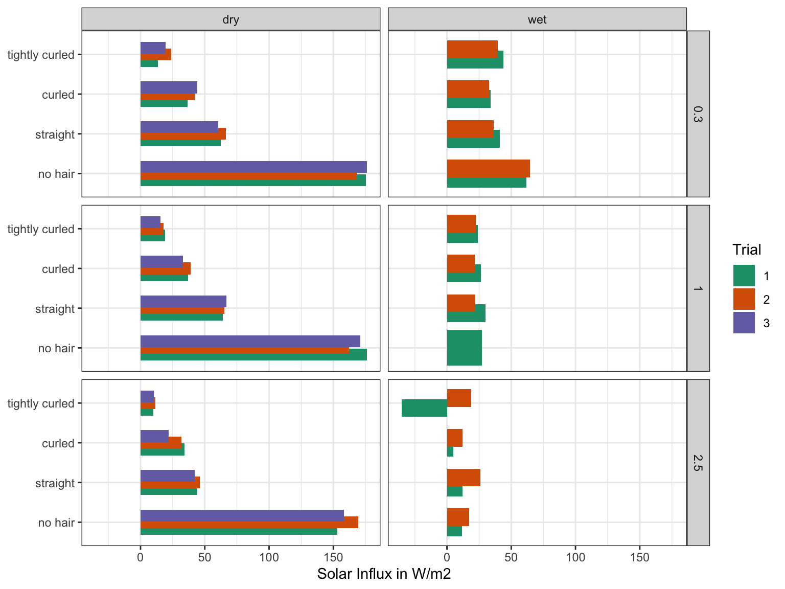
A plot of solar influx shows an outlier in the wet experiments where the heat loss with solar radiation was somehow less than the heat loss without solar radiation. We will exclude this outlier.
df_influx <- df_influx %>%
  mutate(influx = replace(influx, influx<0, NA)) %>%
  drop_na() %>%
  distinct()

write_csv(df_influx, F("data/df_influx.csv"))
1.1.2 Temperature correction (to 30 C)
For the dry heat loss experiments (measuring dry heat resistance), we had to run some experiments at different temperatures to create a large enough gradient between skin/surface temperature and ambient temperature. The manikin is only able to produce results by measuring heat loss, and at 0.3 m/s wind speed, we found that the straight hair and nude (no hair) conditions led to overheating of the manikin. Subsequently, we had to adjust the temperatures to create a temperature gradient.
We thus need to bring all the measurements of heat loss to the same temperature. As heat resistance is temperature independent, we can use this to calculate the expected heat loss at various temperatures. We estimate heat loss at 30C with the following calculation.
\[Heat\ loss (W/m^2)_{(30C\ no\ radiation)} = 5/heat\ resistance_{(no \ radiation)} \]
# take original df imported and filter for values without solar radiation and for dry heat loss only
df_dry_off <- df_wetdry %>%
  filter(radiation=="off" & wet_dry == "dry") %>%
  select(c(wig, wind, wet_dry, resistance, trial)) %>%
  distinct()

df_dry_off| wig | wind | wet_dry | resistance | trial |
|---|---|---|---|---|
| no hair | 0.3 | dry | 0.113 | 1 |
| no hair | 0.3 | dry | 0.112 | 2 |
| no hair | 0.3 | dry | 0.112 | 3 |
| no hair | 1 | dry | 0.099 | 1 |
| no hair | 1 | dry | 0.101 | 2 |
| no hair | 1 | dry | 0.101 | 3 |
| no hair | 2.5 | dry | 0.058 | 1 |
| no hair | 2.5 | dry | 0.056 | 2 |
| no hair | 2.5 | dry | 0.058 | 3 |
| straight | 0.3 | dry | 0.42 | 1 |
| straight | 0.3 | dry | 0.419 | 2 |
| straight | 0.3 | dry | 0.422 | 3 |
| straight | 1 | dry | 0.261 | 1 |
| straight | 1 | dry | 0.27 | 2 |
| straight | 1 | dry | 0.269 | 3 |
| straight | 2.5 | dry | 0.159 | 1 |
| straight | 2.5 | dry | 0.173 | 2 |
| straight | 2.5 | dry | 0.176 | 3 |
| curled | 0.3 | dry | 0.477 | 1 |
| curled | 0.3 | dry | 0.428 | 2 |
| curled | 0.3 | dry | 0.434 | 3 |
| curled | 1 | dry | 0.272 | 1 |
| curled | 1 | dry | 0.286 | 2 |
| curled | 1 | dry | 0.295 | 3 |
| curled | 2.5 | dry | 0.157 | 1 |
| curled | 2.5 | dry | 0.166 | 2 |
| curled | 2.5 | dry | 0.174 | 3 |
| tightly curled | 0.3 | dry | 0.375 | 1 |
| tightly curled | 0.3 | dry | 0.322 | 2 |
| tightly curled | 0.3 | dry | 0.326 | 3 |
| tightly curled | 1 | dry | 0.261 | 1 |
| tightly curled | 1 | dry | 0.265 | 2 |
| tightly curled | 1 | dry | 0.281 | 3 |
| tightly curled | 2.5 | dry | 0.148 | 1 |
| tightly curled | 2.5 | dry | 0.153 | 2 |
| tightly curled | 2.5 | dry | 0.155 | 3 |
# take influx calculated above for dry heat loss and add this as a variable to the df created above for dry heat loss (no radiation). Then calculate the heat loss for 30C using the resistance.
df_dry30_off<- df_influx %>%
  filter(wet_dry == "dry") %>%
  left_join(.,
            df_dry_off) %>%
  mutate(heatloss30 = 5/resistance) %>%
  select(-c(on, off)) %>%
  rename(off = heatloss30) %>%
  distinct()

df_dry30_off| wig | wind | wet_dry | trial | influx | resistance | off |
|---|---|---|---|---|---|---|
| no hair | 0.3 | dry | 1 | 175 | 0.113 | 44.2 |
| no hair | 0.3 | dry | 2 | 168 | 0.112 | 44.6 |
| no hair | 0.3 | dry | 3 | 176 | 0.112 | 44.6 |
| no hair | 1 | dry | 1 | 176 | 0.099 | 50.5 |
| no hair | 1 | dry | 2 | 162 | 0.101 | 49.5 |
| no hair | 1 | dry | 3 | 171 | 0.101 | 49.5 |
| no hair | 2.5 | dry | 1 | 153 | 0.058 | 86.2 |
| no hair | 2.5 | dry | 2 | 169 | 0.056 | 89.3 |
| no hair | 2.5 | dry | 3 | 158 | 0.058 | 86.2 |
| straight | 0.3 | dry | 1 | 62.6 | 0.42 | 11.9 |
| straight | 0.3 | dry | 2 | 66.3 | 0.419 | 11.9 |
| straight | 0.3 | dry | 3 | 60.3 | 0.422 | 11.8 |
| straight | 1 | dry | 1 | 64.2 | 0.261 | 19.2 |
| straight | 1 | dry | 2 | 65.1 | 0.27 | 18.5 |
| straight | 1 | dry | 3 | 66.8 | 0.269 | 18.6 |
| straight | 2.5 | dry | 1 | 44.1 | 0.159 | 31.4 |
| straight | 2.5 | dry | 2 | 46.2 | 0.173 | 28.9 |
| straight | 2.5 | dry | 3 | 42.2 | 0.176 | 28.4 |
| curled | 0.3 | dry | 1 | 36.4 | 0.477 | 10.5 |
| curled | 0.3 | dry | 2 | 42 | 0.428 | 11.7 |
| curled | 0.3 | dry | 3 | 44.1 | 0.434 | 11.5 |
| curled | 1 | dry | 1 | 36.8 | 0.272 | 18.4 |
| curled | 1 | dry | 2 | 38.8 | 0.286 | 17.5 |
| curled | 1 | dry | 3 | 33 | 0.295 | 16.9 |
| curled | 2.5 | dry | 1 | 34.1 | 0.157 | 31.8 |
| curled | 2.5 | dry | 2 | 31.9 | 0.166 | 30.1 |
| curled | 2.5 | dry | 3 | 21.8 | 0.174 | 28.7 |
| tightly curled | 0.3 | dry | 1 | 13.5 | 0.375 | 13.3 |
| tightly curled | 0.3 | dry | 2 | 23.8 | 0.322 | 15.5 |
| tightly curled | 0.3 | dry | 3 | 19.5 | 0.326 | 15.3 |
| tightly curled | 1 | dry | 1 | 19.1 | 0.261 | 19.2 |
| tightly curled | 1 | dry | 2 | 17.8 | 0.265 | 18.9 |
| tightly curled | 1 | dry | 3 | 15.6 | 0.281 | 17.8 |
| tightly curled | 2.5 | dry | 1 | 9.9 | 0.148 | 33.8 |
| tightly curled | 2.5 | dry | 2 | 11.5 | 0.153 | 32.7 |
| tightly curled | 2.5 | dry | 3 | 10.4 | 0.155 | 32.3 |
To calculate the heat loss at 30C with radiation, we subtract the solar influx from the temperature corrected heat loss:
\[Heat\ loss (W/m^2)_{(30C\ with\ radiation)} = Heat\ loss (W/m^2)_{(30C\ no\ radiation)}- solar\ influx(W/m^2) \]
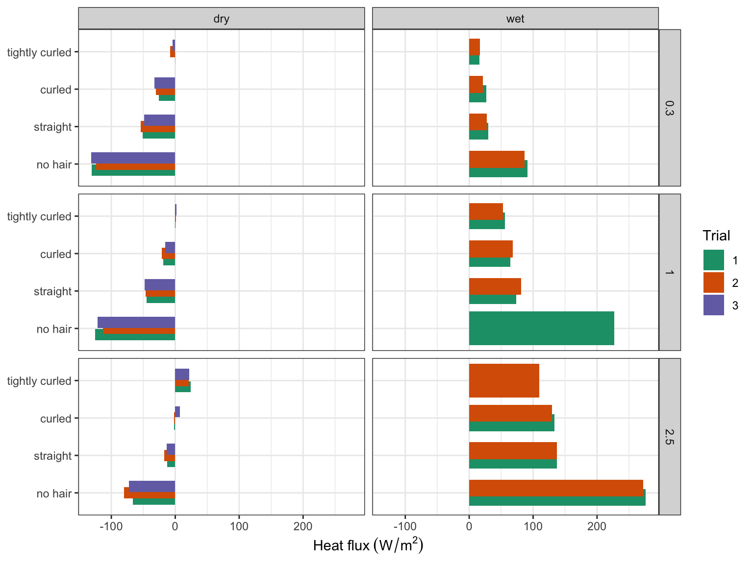
Dry heat loss at 30C and isothermal wet heat loss with radiation on
| Version | Author | Date |
|---|---|---|
| bf62a07 | Tina Lasisi | 2022-03-10 |
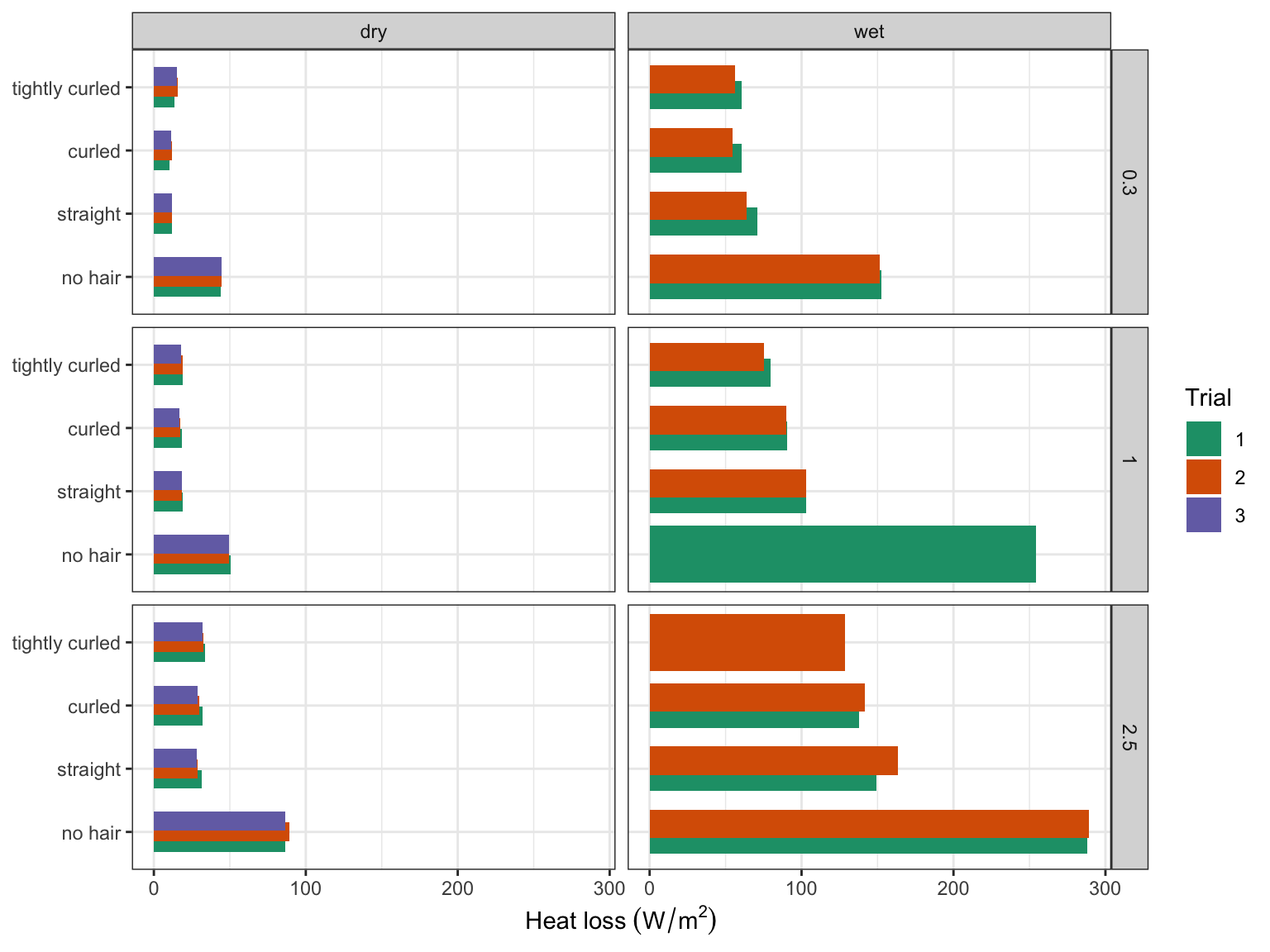
Dry heat loss at 30C and isothermal wet heat loss with radiation off
| Version | Author | Date |
|---|---|---|
| bf62a07 | Tina Lasisi | 2022-03-10 |
2 Exploratory plots
Here we show the combined heat loss for wet heat loss and and dry heat loss
The calculation of these combined values is as follows:
\[Combined \ heat\ loss (W/m^2)_{(30C\ wet+dry + no \ radiation)} = Dry\ heat\ loss (W/m^2)_{(30C\ no\ radiation)} + Wet\ heat\ loss (W/m^2)_{(30C\ no\ radiation)} \]
\[Combined \ heat\ loss (W/m^2)_{(30C\ wet+dry + radiation)} = Dry\ heat\ loss (W/m^2)_{(30C\ no\ radiation)} + Wet\ heat\ loss (W/m^2)_{(30C\ + radiation)} \] \[Combined \ influx (W/m^2)_{(30C\ wet+dry)} = Combined \ heat\ loss (W/m^2)_{(30C\ wet+dry + no \ radiation)} - Combined \ heat\ loss (W/m^2)_{(30C\ wet+dry + radiation)} \]
# A tibble: 6 × 6
# Groups:   wig, wind [2]
  wig      wind var     mean   max   min
  <fct>   <dbl> <chr>  <dbl> <dbl> <dbl>
1 no hair   0.3 off    197.  197.  196.
2 no hair   0.3 on     133.  136.  131.
3 no hair   0.3 influx  63.3  61.9  64.7
4 no hair   1   off    304.  305.  304.
5 no hair   1   on     277.  278.  277.
6 no hair   1   influx  27.2  27.2  27.2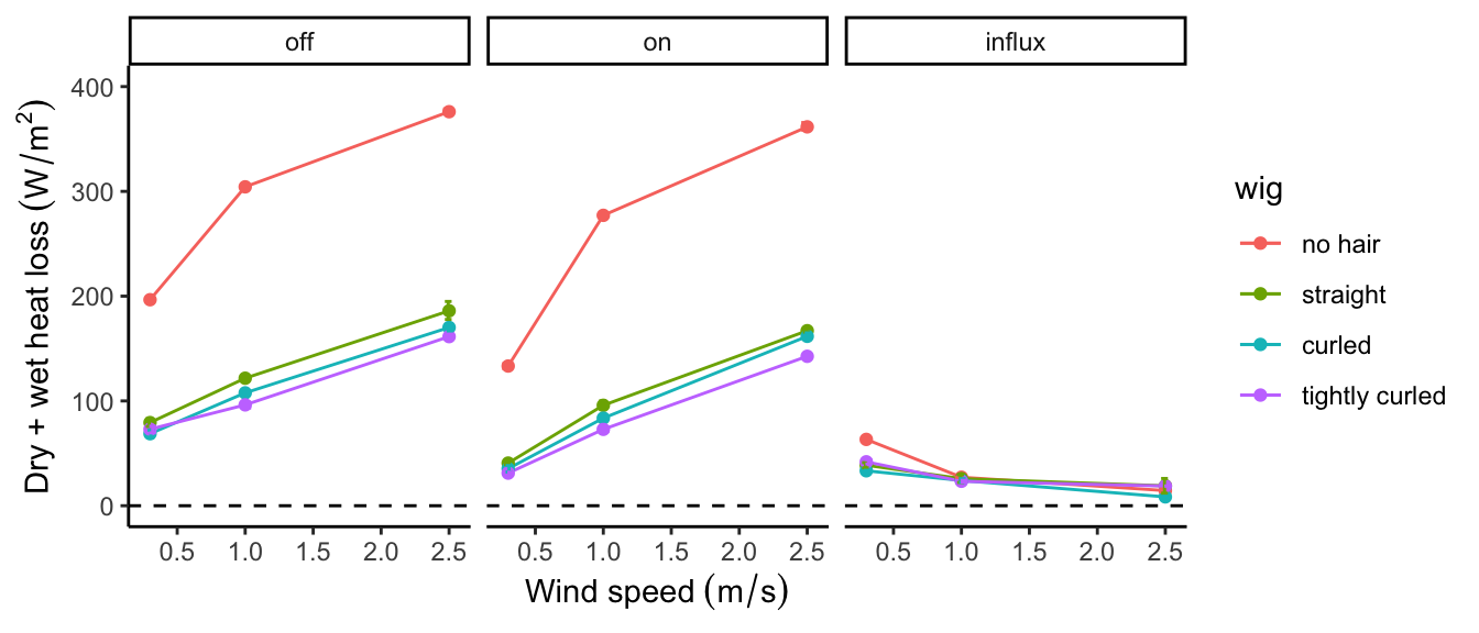
2.1 Sweating
We use the dry and wet data to infer the amount of sweat that a scalp could evaporate under conditions of solar radiation at 30C (maximum sweat capacity) and how much evaporative cooling from sweat would be needed to cancel out any heat gain (zero heat gain sweat).
Here, we plot the sweat rate potential (left) and the sweat rate required to cancel out heat gain at \(T_{ambient} = 30^\circ C\).
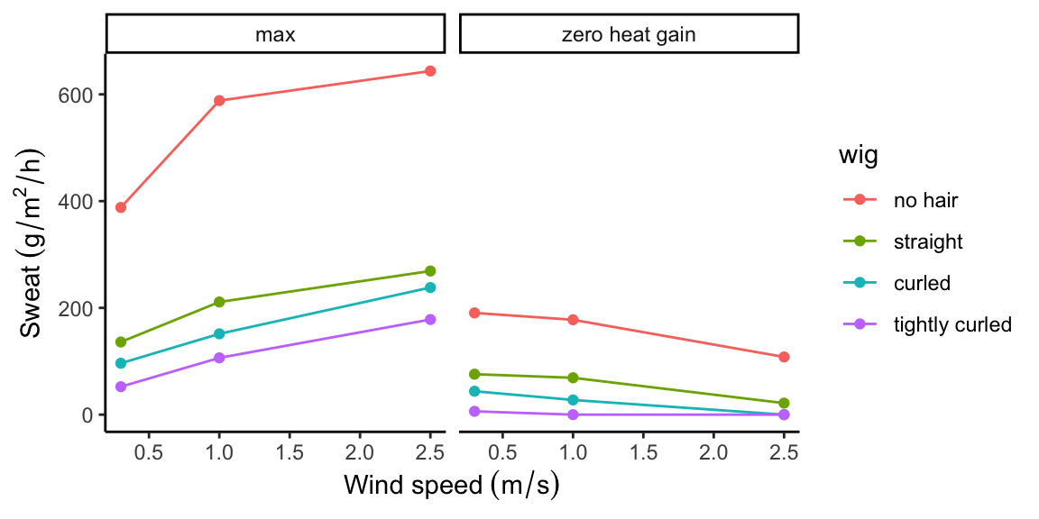
The quantity of sweat that can be maximally evaporated (left) and that is required for zero heat gain (right) with various head coverings under three wind speeds
What emerges is that while heat loss potential is higher without hair as a barrier (i.e. the “nude” condition), the potential sweat far exceeds the physiologically possible sweat rate for humans. The plot for zero heat gain shoes that a nude scalp requires the most sweat and this requirement is inversely correlated with hair curvature.
3 Regression models
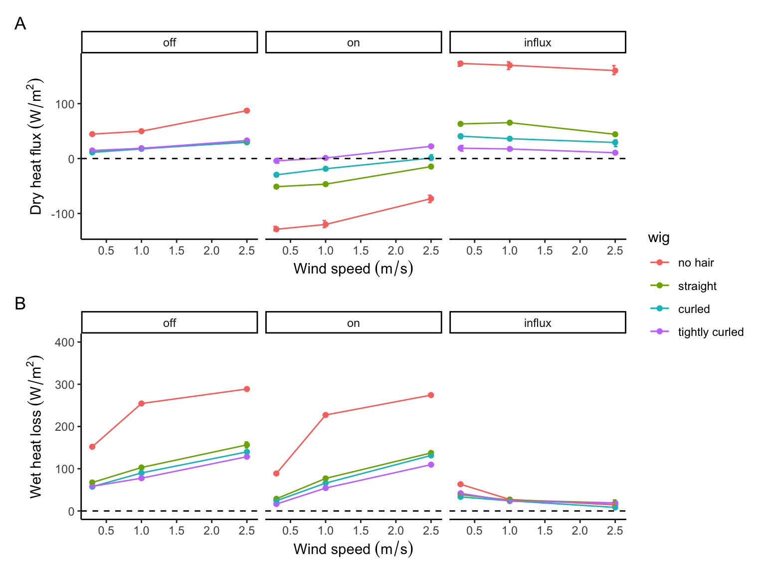
3.1 Dry heat loss
3.1.1 Radiation off
Here, we model the effect of the wig variable on the off (heat loss without radiation) variable while correcting for wind.
Without radiation, having hair will reduce the heat loss.
Call:
lm(formula = off ~ wind + wig, data = df_dry_off)

Residuals:
    Min      1Q  Median      3Q     Max
-8.0046 -4.0646  0.1855  2.7241 14.8000

Coefficients:
                  Estimate Std. Error t value Pr(>|t|)
(Intercept)         46.192      2.279   20.27  < 2e-16 ***
wind                11.317      1.022   11.07 2.65e-12 ***
wigstraight        -40.449      2.653  -15.25 5.91e-16 ***
wigcurled          -40.838      2.653  -15.39 4.54e-16 ***
wigtightly curled  -38.445      2.653  -14.49 2.37e-15 ***
---
Signif. codes:  0 '***' 0.001 '**' 0.01 '*' 0.05 '.' 0.1 ' ' 1

Residual standard error: 5.627 on 31 degrees of freedom
Multiple R-squared:  0.9373,    Adjusted R-squared:  0.9292
F-statistic: 115.8 on 4 and 31 DF,  p-value: < 2.2e-16
3.1.2 Radiation on
With radiation, there is a net increase in heat (i.e. heat gain) without any hair. Additonally, we observe that heat gain decreases with increasingly curled hair.
Call:
lm(formula = on ~ wind + wig, data = df_dry_on)

Residuals:
     Min       1Q   Median       3Q      Max
-13.6579  -4.8720  -0.0048   3.3664  18.9682

Coefficients:
                  Estimate Std. Error t value Pr(>|t|)
(Intercept)       -129.287      2.854  -45.29  < 2e-16 ***
wind                17.450      1.280   13.63 1.23e-14 ***
wigstraight         69.729      3.322   20.99  < 2e-16 ***
wigcurled           91.439      3.322   27.52  < 2e-16 ***
wigtightly curled  113.588      3.322   34.19  < 2e-16 ***
---
Signif. codes:  0 '***' 0.001 '**' 0.01 '*' 0.05 '.' 0.1 ' ' 1

Residual standard error: 7.048 on 31 degrees of freedom
Multiple R-squared:  0.9798,    Adjusted R-squared:  0.9771
F-statistic:   375 on 4 and 31 DF,  p-value: < 2.2e-16
3.1.3 Solar influx
Here, we model the effect of the wig variable on influx while correcting for wind.
In the dry heat loss experiments, we see that all hair (regardless of curliness) decreases the solar influx. Additionally, the curlier the hair, the lower the solar influx.
Call:
lm(formula = influx ~ wind + wig, data = df_dry)
Residuals:
Min 1Q Median 3Q Max
-8.106 -3.844 1.099 2.763 9.053
Coefficients:
Estimate Std. Error t value Pr(>|t|)
(Intercept) 175.4796 2.0111 87.254 < 2e-16 ***
wind -6.1330 0.9018 -6.801 1.29e-07 ***
wigstraight -110.1778 2.3409 -47.067 < 2e-16 ***
wigcurled -132.2778 2.3409 -56.508 < 2e-16 ***
wigtightly curled -152.0333 2.3409 -64.948 < 2e-16 ***
---
Signif. codes: 0 '***' 0.001 '**' 0.01 '*' 0.05 '.' 0.1 ' ' 1
Residual standard error: 4.966 on 31 degrees of freedom
Multiple R-squared: 0.994, Adjusted R-squared: 0.9932
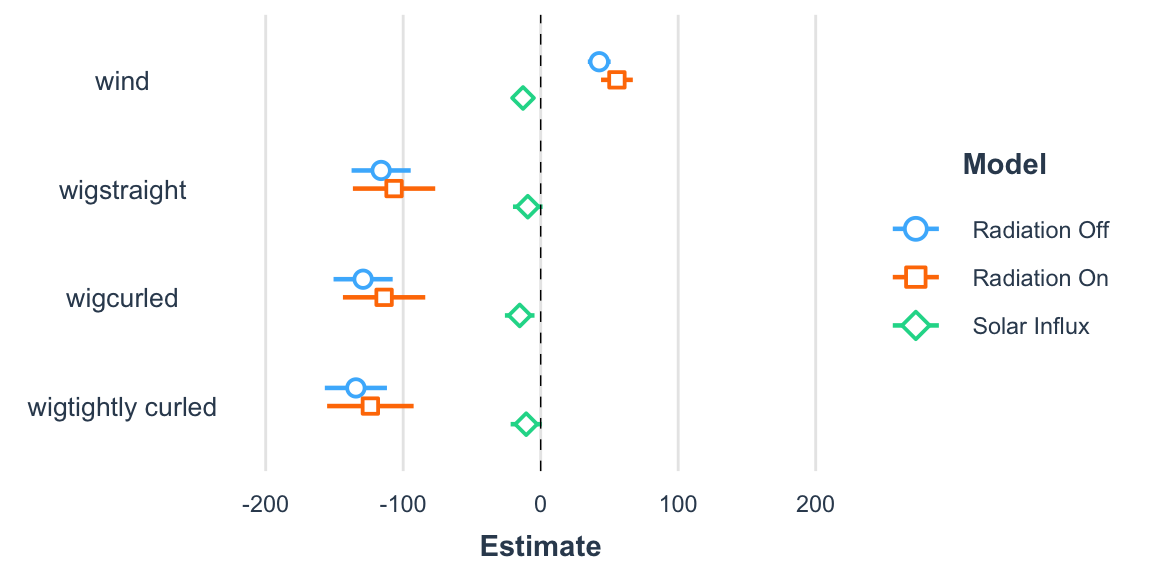
F-statistic: 1275 on 4 and 31 DF, p-value: < 2.2e-163.1.4 Summary of dry heat loss regression models
3.1.4.1 All separate
| Radiation Off | Radiation On | Solar Influx | |
|---|---|---|---|
| (Intercept) | 46.19 *** | -129.29 *** | 175.48 *** |
| [41.54, 50.84] | [-135.11, -123.47] | [171.38, 179.58] | |
| wind | 11.32 *** | 17.45 *** | -6.13 *** |
| [9.23, 13.40] | [14.84, 20.06] | [-7.97, -4.29] | |
| wigstraight | -40.45 *** | 69.73 *** | -110.18 *** |
| [-45.86, -35.04] | [62.95, 76.50] | [-114.95, -105.40] | |
| wigcurled | -40.84 *** | 91.44 *** | -132.28 *** |
| [-46.25, -35.43] | [84.66, 98.22] | [-137.05, -127.50] | |
| wigtightly curled | -38.45 *** | 113.59 *** | -152.03 *** |
| [-43.86, -33.04] | [106.81, 120.36] | [-156.81, -147.26] | |
| N | 36 | 36 | 36 |
| R2 | 0.94 | 0.98 | 0.99 |
| *** p < 0.001; ** p < 0.01; * p < 0.05. | |||
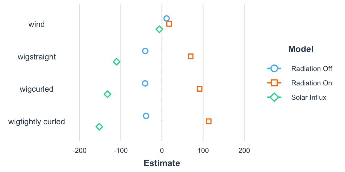
Regression coefficients across regression models.
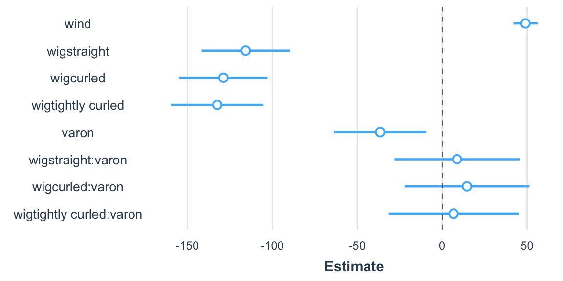
3.1.4.2 Radiation conditions combined
Call:
lm(formula = heatloss ~ wind + wig + var + var * wig, data = df_dry_radcombo)

Residuals:
     Min       1Q   Median       3Q      Max
-14.4757  -4.5094  -0.4139   4.7580  22.7503

Coefficients:
                         Estimate Std. Error t value Pr(>|t|)
(Intercept)               42.3079     2.5983   16.28   <2e-16 ***
wind                      14.3839     0.8996   15.99   <2e-16 ***
wigstraight              -40.4490     3.3023  -12.25   <2e-16 ***
wigcurled                -40.8384     3.3023  -12.37   <2e-16 ***
wigtightly curled        -38.4455     3.3023  -11.64   <2e-16 ***
varon                   -167.7111     3.3023  -50.79   <2e-16 ***
wigstraight:varon        110.1778     4.6702   23.59   <2e-16 ***
wigcurled:varon          132.2778     4.6702   28.32   <2e-16 ***
wigtightly curled:varon  152.0333     4.6702   32.55   <2e-16 ***
---
Signif. codes:  0 '***' 0.001 '**' 0.01 '*' 0.05 '.' 0.1 ' ' 1

Residual standard error: 7.005 on 63 degrees of freedom
Multiple R-squared:  0.9826,    Adjusted R-squared:  0.9804
F-statistic: 444.5 on 8 and 63 DF, p-value: < 2.2e-16| Model 1 | |
|---|---|
| (Intercept) | 42.31 *** |
| [37.12, 47.50] | |
| wind | 14.38 *** |
| [12.59, 16.18] | |
| wigstraight | -40.45 *** |
| [-47.05, -33.85] | |
| wigcurled | -40.84 *** |
| [-47.44, -34.24] | |
| wigtightly curled | -38.45 *** |
| [-45.04, -31.85] | |
| varon | -167.71 *** |
| [-174.31, -161.11] | |
| wigstraight:varon | 110.18 *** |
| [100.85, 119.51] | |
| wigcurled:varon | 132.28 *** |
| [122.95, 141.61] | |
| wigtightly curled:varon | 152.03 *** |
| [142.70, 161.37] | |
| N | 72 |
| R2 | 0.98 |
| *** p < 0.001; ** p < 0.01; * p < 0.05. | |
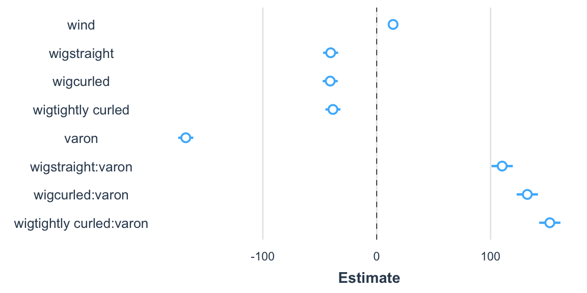
Regression coefficients for dry heatloss
3.2 Evaporative resistance (wet experiments)
Here, we repeat the same modelling process for the evaporative resistance data from the wet experiments.
3.2.1 Radiation off
Here, we model the effect of the wig variable on the off (heat loss without radiation) variable while correcting for wind.
Without solar radiation, all hair (regardless of texture) decreases evaporative resistance.
Call:
lm(formula = off ~ wind + wig, data = df_wet_off)

Residuals:
    Min      1Q  Median      3Q     Max
-32.423  -5.988   2.672   5.875  40.867

Coefficients:
                  Estimate Std. Error t value Pr(>|t|)
(Intercept)        171.047      9.142   18.71 8.88e-13 ***
wind                42.586      3.933   10.83 4.77e-09 ***
wigstraight       -116.039     10.191  -11.39 2.24e-09 ***
wigcurled         -129.155     10.191  -12.67 4.35e-10 ***
wigtightly curled -134.404     10.707  -12.55 5.04e-10 ***
---
Signif. codes:  0 '***' 0.001 '**' 0.01 '*' 0.05 '.' 0.1 ' ' 1

Residual standard error: 16.83 on 17 degrees of freedom
Multiple R-squared:  0.955, Adjusted R-squared:  0.9444
F-statistic: 90.24 on 4 and 17 DF,  p-value: 3.238e-11
3.2.2 Radiation on
With radiation, hair decreases evaporative resistance.
Call:
lm(formula = on ~ wind + wig, data = df_wet_on)

Residuals:
    Min      1Q  Median      3Q     Max
-47.469 -11.283   4.403   6.848  54.322

Coefficients:
                  Estimate Std. Error t value Pr(>|t|)
(Intercept)        117.536     12.729   9.234 4.91e-08 ***
wind                55.442      5.476  10.124 1.29e-08 ***
wigstraight       -106.646     14.189  -7.516 8.45e-07 ***
wigcurled         -113.896     14.189  -8.027 3.49e-07 ***
wigtightly curled -123.867     14.908  -8.309 2.17e-07 ***
---
Signif. codes:  0 '***' 0.001 '**' 0.01 '*' 0.05 '.' 0.1 ' ' 1

Residual standard error: 23.43 on 17 degrees of freedom
Multiple R-squared:  0.9255,    Adjusted R-squared:  0.9079
F-statistic: 52.77 on 4 and 17 DF,  p-value: 2.307e-09
3.2.3 Solar influx
Combining the above data to calculate solar influx, we see that there is not a considerable effect of radiation on evaporative resistance.
Call:
lm(formula = influx ~ wind + wig, data = df_wet)

Residuals:
     Min       1Q   Median       3Q      Max
-13.4541  -4.2173  -0.8525   3.9887  15.0463

Coefficients:
                  Estimate Std. Error t value Pr(>|t|)
(Intercept)         53.511      4.577  11.690 1.50e-09 ***
wind               -12.857      1.969  -6.529 5.15e-06 ***
wigstraight         -9.392      5.102  -1.841  0.08318 .
wigcurled          -15.259      5.102  -2.991  0.00822 **
wigtightly curled  -10.537      5.361  -1.966  0.06591 .
---
Signif. codes:  0 '***' 0.001 '**' 0.01 '*' 0.05 '.' 0.1 ' ' 1

Residual standard error: 8.425 on 17 degrees of freedom
Multiple R-squared:  0.7498,    Adjusted R-squared:  0.6909
F-statistic: 12.74 on 4 and 17 DF,  p-value: 5.664e-05
3.2.4 Summary of evaporative heat loss regression models
3.2.4.1 All separate
| Radiation Off | Radiation On | Solar Influx | |
|---|---|---|---|
| (Intercept) | 171.05 *** | 117.54 *** | 53.51 *** |
| [151.76, 190.34] | [90.68, 144.39] | [43.85, 63.17] | |
| wind | 42.59 *** | 55.44 *** | -12.86 *** |
| [34.29, 50.88] | [43.89, 67.00] | [-17.01, -8.70] | |
| wigstraight | -116.04 *** | -106.65 *** | -9.39 |
| [-137.54, -94.54] | [-136.58, -76.71] | [-20.16, 1.37] | |
| wigcurled | -129.16 *** | -113.90 *** | -15.26 ** |
| [-150.66, -107.65] | [-143.83, -83.96] | [-26.02, -4.49] | |
| wigtightly curled | -134.40 *** | -123.87 *** | -10.54 |
| [-157.00, -111.81] | [-155.32, -92.41] | [-21.85, 0.77] | |
| N | 22 | 22 | 22 |
| R2 | 0.96 | 0.93 | 0.75 |
| *** p < 0.001; ** p < 0.01; * p < 0.05. | |||
Regression coefficients across regression models.
3.2.4.2 Radiation conditions combined
Call:
lm(formula = heatloss ~ wind + wig + var + var * wig, data = df_wet_radcombo)

Residuals:
    Min      1Q  Median      3Q     Max
-54.026  -5.065   1.900   7.208  52.264

Coefficients:
                        Estimate Std. Error t value Pr(>|t|)
(Intercept)              162.561     10.524  15.446  < 2e-16 ***
wind                      49.014      3.496  14.021 6.29e-16 ***
wigstraight             -115.696     12.808  -9.033 1.13e-10 ***
wigcurled               -128.813     12.808 -10.057 7.31e-12 ***
wigtightly curled       -132.476     13.418  -9.873 1.18e-11 ***
varon                    -36.540     13.377  -2.732  0.00981 **
wigstraight:varon          8.707     18.112   0.481  0.63371
wigcurled:varon           14.573     18.112   0.805  0.42647
wigtightly curled:varon    6.680     18.917   0.353  0.72612
---
Signif. codes:  0 '***' 0.001 '**' 0.01 '*' 0.05 '.' 0.1 ' ' 1

Residual standard error: 21.15 on 35 degrees of freedom
Multiple R-squared:  0.9351,    Adjusted R-squared:  0.9203
F-statistic: 63.04 on 8 and 35 DF, p-value: < 2.2e-16| Model 1 | |
|---|---|
| (Intercept) | 162.56 *** |
| [141.20, 183.93] | |
| wind | 49.01 *** |
| [41.92, 56.11] | |
| wigstraight | -115.70 *** |
| [-141.70, -89.69] | |
| wigcurled | -128.81 *** |
| [-154.82, -102.81] | |
| wigtightly curled | -132.48 *** |
| [-159.71, -105.24] | |
| varon | -36.54 ** |
| [-63.70, -9.38] | |
| wigstraight:varon | 8.71 |
| [-28.06, 45.48] | |
| wigcurled:varon | 14.57 |
| [-22.20, 51.34] | |
| wigtightly curled:varon | 6.68 |
| [-31.72, 45.08] | |
| N | 44 |
| R2 | 0.94 |
| *** p < 0.001; ** p < 0.01; * p < 0.05. | |
Regression coefficients for evaporative heatloss
R version 4.1.2 (2021-11-01)
Platform: x86_64-apple-darwin17.0 (64-bit)
Running under: macOS Big Sur 10.16

Matrix products: default
BLAS:   /Library/Frameworks/R.framework/Versions/4.1/Resources/lib/libRblas.0.dylib
LAPACK: /Library/Frameworks/R.framework/Versions/4.1/Resources/lib/libRlapack.dylib

locale:
[1] en_US.UTF-8/en_US.UTF-8/en_US.UTF-8/C/en_US.UTF-8/en_US.UTF-8

attached base packages:
[1] stats     graphics  grDevices utils     datasets  methods   base

other attached packages:
 [1] huxtable_5.4.0    broom.mixed_0.2.7 gtsummary_1.5.2   jtools_2.1.4
 [5] patchwork_1.1.1   gridExtra_2.3     ggstatsplot_0.9.0 fs_1.5.2
 [9] kableExtra_1.3.4  knitr_1.37        forcats_0.5.1     stringr_1.4.0
[13] dplyr_1.0.8       purrr_0.3.4       readr_2.0.2       tidyr_1.1.4
[17] tibble_3.1.6      ggplot2_3.3.5     tidyverse_1.3.1   workflowr_1.6.2

loaded via a namespace (and not attached):
  [1] colorspace_2.0-2       ellipsis_0.3.2         rprojroot_2.0.2
  [4] ggstance_0.3.5         parameters_0.15.0      mc2d_0.1-21
  [7] rstudioapi_0.13        farver_2.1.0           bit64_4.0.5
 [10] fansi_0.5.0            mvtnorm_1.1-3          lubridate_1.8.0
 [13] xml2_1.3.2             splines_4.1.2          cachem_1.0.6
 [16] SuppDists_1.1-9.5      zeallot_0.1.0          jsonlite_1.7.2
 [19] gt_0.4.0               broom_0.7.12           Rmpfr_0.8-7
 [22] dbplyr_2.1.1           compiler_4.1.2         httr_1.4.2
 [25] PMCMRplus_1.9.3        backports_1.2.1        assertthat_0.2.1
 [28] fastmap_1.1.0          cli_3.2.0              later_1.3.0
 [31] htmltools_0.5.2        tools_4.1.2            gmp_0.6-2.1
 [34] gtable_0.3.0           glue_1.6.2             Rcpp_1.0.7
 [37] cellranger_1.1.0       jquerylib_0.1.4        vctrs_0.3.8
 [40] svglite_2.0.0          nlme_3.1-153           broom.helpers_1.6.0
 [43] insight_0.14.5         xfun_0.29              rvest_1.0.2
 [46] lifecycle_1.0.1        MASS_7.3-54            scales_1.1.1
 [49] vroom_1.5.5            hms_1.1.1              promises_1.2.0.1
 [52] parallel_4.1.2         RColorBrewer_1.1-2     rematch2_2.1.2
 [55] yaml_2.2.1             memoise_2.0.0          pander_0.6.4
 [58] reshape_0.8.8          stringi_1.7.5          highr_0.9
 [61] paletteer_1.4.0        bayestestR_0.11.5      commonmark_1.7
 [64] rlang_1.0.2            pkgconfig_2.0.3        systemfonts_1.0.3
 [67] evaluate_0.14          lattice_0.20-45        labeling_0.4.2
 [70] bit_4.0.4              tidyselect_1.1.1       plyr_1.8.6
 [73] magrittr_2.0.2         R6_2.5.1               generics_0.1.0
 [76] multcompView_0.1-8     BWStest_0.2.2          DBI_1.1.1
 [79] pillar_1.6.4           haven_2.4.3            whisker_0.4
 [82] withr_2.4.2            datawizard_0.2.1       performance_0.8.0
 [85] modelr_0.1.8           crayon_1.4.1           WRS2_1.1-3
 [88] utf8_1.2.2             correlation_0.7.1      tzdb_0.1.2
 [91] rmarkdown_2.11         kSamples_1.2-9         grid_4.1.2
 [94] readxl_1.3.1           git2r_0.28.0           reprex_2.0.1
 [97] digest_0.6.28          webshot_0.5.2          httpuv_1.6.3
[100] statsExpressions_1.2.0 munsell_0.5.0          viridisLite_0.4.0