Analyses

Last updated: 2023-03-06

Checks: 6 1

Knit directory: PODFRIDGE/

This reproducible R Markdown analysis was created with workflowr (version 1.7.0). The Checks tab describes the reproducibility checks that were applied when the results were created. The Past versions tab lists the development history.

R Markdown file: uncommitted changes

The R Markdown file has unstaged changes. To know which version of the R Markdown file created these results, you’ll want to first commit it to the Git repo. If you’re still working on the analysis, you can ignore this warning. When you’re finished, you can run wflow_publish to commit the R Markdown file and build the HTML.

Environment: empty

Great job! The global environment was empty. Objects defined in the global environment can affect the analysis in your R Markdown file in unknown ways. For reproduciblity it’s best to always run the code in an empty environment.

Seed: set.seed(20230302)

The command set.seed(20230302) was run prior to running the code in the R Markdown file. Setting a seed ensures that any results that rely on randomness, e.g. subsampling or permutations, are reproducible.

Session information: recorded

Great job! Recording the operating system, R version, and package versions is critical for reproducibility.

Cache: none

Nice! There were no cached chunks for this analysis, so you can be confident that you successfully produced the results during this run.

File paths: relative

Great job! Using relative paths to the files within your workflowr project makes it easier to run your code on other machines.

Repository version: 5f805fe

Great! You are using Git for version control. Tracking code development and connecting the code version to the results is critical for reproducibility.

The results in this page were generated with repository version 5f805fe. See the Past versions tab to see a history of the changes made to the R Markdown and HTML files.

Note that you need to be careful to ensure that all relevant files for the analysis have been committed to Git prior to generating the results (you can use wflow_publish or wflow_git_commit). workflowr only checks the R Markdown file, but you know if there are other scripts or data files that it depends on. Below is the status of the Git repository when the results were generated:


Ignored files:
    Ignored:    .DS_Store
    Ignored:    .Rproj.user/
    Ignored:    data/.DS_Store

Unstaged changes:
    Modified:   analysis/analyses.Rmd
    Modified:   analysis/methods.Rmd
    Modified:   data/us-pop-detailed-multisheet.xls

Note that any generated files, e.g. HTML, png, CSS, etc., are not included in this status report because it is ok for generated content to have uncommitted changes.

These are the previous versions of the repository in which changes were made to the R Markdown (analysis/analyses.Rmd) and HTML (docs/analyses.html) files. If you’ve configured a remote Git repository (see ?wflow_git_remote), click on the hyperlinks in the table below to view the files as they were in that past version.

File	Version	Author	Date	Message
html	5f805fe	Tina Lasisi	2023-03-05	Build site.
Rmd	5106bab	Tina Lasisi	2023-03-05	add analyses
html	c3948af	Tina Lasisi	2023-03-04	Build site.
html	f02bc38	Tina Lasisi	2023-03-02	Build site.
html	c9130d5	Tina Lasisi	2023-03-02	wflow_git_commit(all = TRUE)
html	a4a7d45	Tina Lasisi	2023-03-02	Build site.
html	00073fd	Tina Lasisi	2023-03-02	Build site.
html	51ed5a6	Tina Lasisi	2023-03-02	Build site.
Rmd	13ed9ae	Tina Lasisi	2023-03-02	Publishing POPFORGE
html	13ed9ae	Tina Lasisi	2023-03-02	Publishing POPFORGE

# Load necessary packages
library(wesanderson) # for color palettes
library(tidyverse) #data wrangling etc

── Attaching packages ─────────────────────────────────────── tidyverse 1.3.2 ──
✔ ggplot2 3.4.0      ✔ purrr   0.3.5 
✔ tibble  3.1.8      ✔ dplyr   1.0.10
✔ tidyr   1.2.1      ✔ stringr 1.5.0 
✔ readr   2.1.3      ✔ forcats 0.5.2 
── Conflicts ────────────────────────────────────────── tidyverse_conflicts() ──
✖ dplyr::filter() masks stats::filter()
✖ dplyr::lag()    masks stats::lag()

# Set path to the data file
path <- "./data/"
savepath <- "./output/"

# Set up vector for cousin degree
p <- c(1:8) 

# Set up initial population size
N <- 76e6 

# Read in data on US population sizes by year
US_pop <- read.csv(paste(path, "est-pop-combo.csv", sep = ""))

# Calculate number of grandparents by generation
p_grandpar_gen <- 1990 - 30 * (p + 1)

# Get population sizes by year for grandparents' generation

US_Ns <- US_pop %>% 
  filter(Year %in% p_grandpar_gen)

# Scale population size down by 50% (assumed number of potential parents) and 90% of those have children + set minimum for populations

# US_Ns %>% 
#   mutate(across(!Year, ~ . * 0.5 * 0.9))

N <- US_Ns %>% 
  mutate(across(!Year, ~ case_when(. * 0.5 * 0.9 < 1e6 ~ 1e6,
                                   TRUE ~ . * 0.5 * 0.9)))

# Set up vector of database sizes to test
DB.sizes <- c(1e6, 5e6, 10e6)

DB.sizes.EUR <- DB.sizes*0.8
DB.sizes.AFR <- DB.sizes*0.05

# Set color palette for graphs
my.cols <- wes_palette("Darjeeling1")

  Year    Total    White   Black
1 1720  1000000  1000000 1000000
2 1750  1000000  1000000 1000000
3 1780  1251166  1000000 1000000
4 1810  3257946  2637933 1000000
5 1840  7678509  6385367 1293142
6 1870 17351267 15115220 2196004
7 1900 34197559 30064138 3975297
8 1930 55248771 49629033 5351014

Probability of p-th degree cousin

plot_prob_DB_size <- function(p, DB.sizes, N, my.cols) {
  plot(c(1, 8), c(0, 1), type = "n", ylab = "Probability of at least one p-th cousin in database", xlab = "p (degree of cousin)")
  sapply(1:length(DB.sizes), function(i) {
    DB.size <- DB.sizes[i]
    prob.no.rellys <- exp(-2^(2*p - 2) * DB.size / N)
    points(p, 1 - prob.no.rellys, type = "b", col = my.cols[i], pch = 19, lwd = 1.5)
  })
  legend(x = "bottomright", legend = c("Database size (Millions) =", format(DB.sizes / 1e6, dig = 1)), col = c(NA, my.cols), pch = 19)
}

layout(t(1:2))

# plot_prob_DB_size(p, DB.sizes.EUR, N$Total,  my.cols)
plot_prob_DB_size(p, DB.sizes.EUR, N$White,  my.cols)
# plot_prob_DB_size(p, DB.sizes.EUR, N$White,  my.cols)
# plot_prob_DB_size(p, DB.sizes.EUR, N$Total,  my.cols)
plot_prob_DB_size(p, DB.sizes.AFR, N$Black,  my.cols)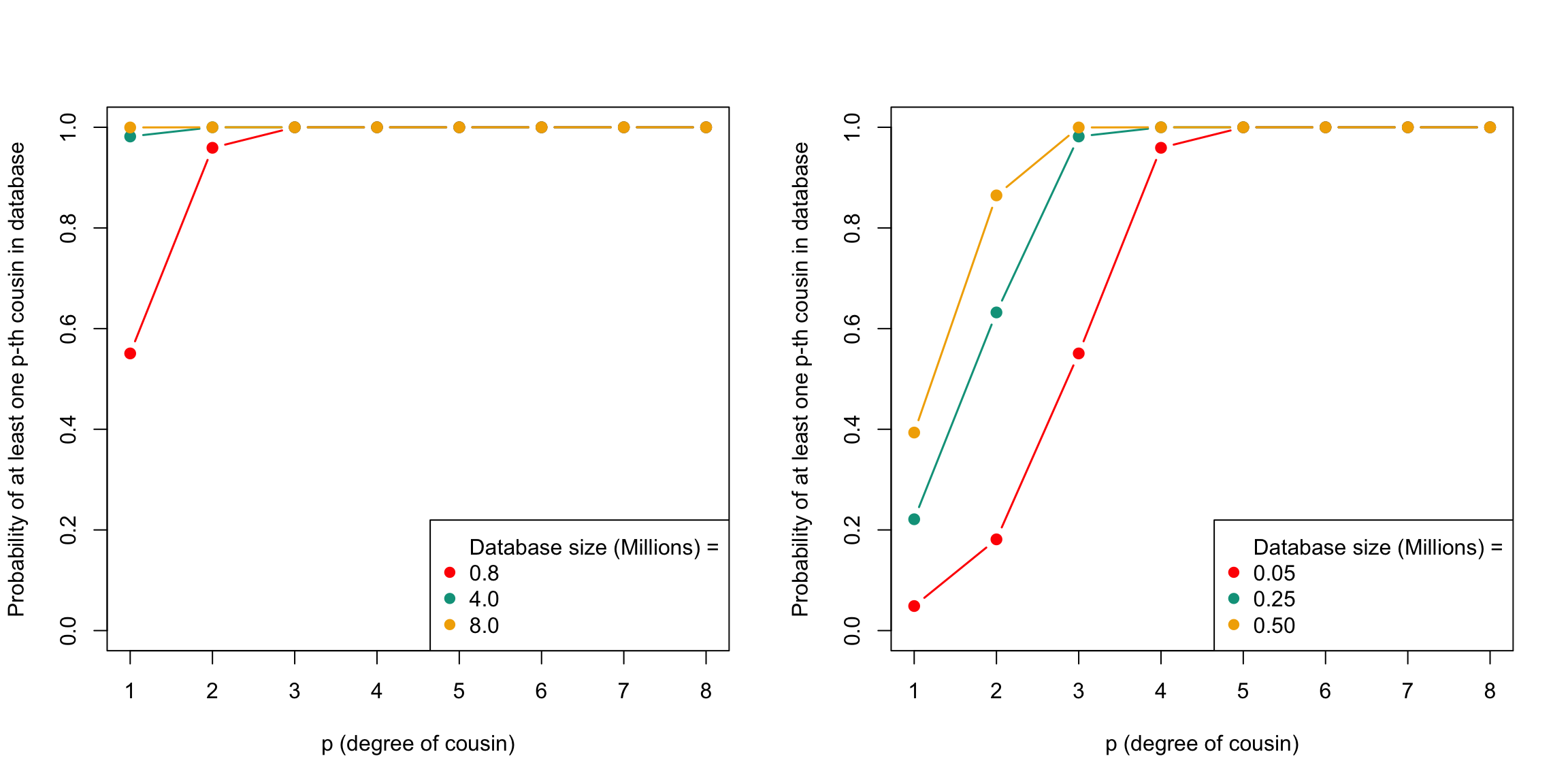

The plot above displays the probability of having at least one p-th cousin in a genetic database and the expected number of p-th cousins in a database. The plot shows the probability of finding at least one p-th cousin in a database of a given size for White Americans (left) and Black Americans (right)

Version	Author	Date
5f805fe	Tina Lasisi	2023-03-05

# plot_prob_DB_size(p, DB.sizes.AFR, N$Total,  my.cols)

Number of p-th degree cousins

# Plot of expected number of p-th cousins in sample
expected_cousins <- function(p, DB.sizes, N, my.cols) {
  plot(c(1,8), c(0,1000), type = "n", ylab = "Expected number of p-th cousins in database", xlab = "p.(degree of cousin)")
  sapply(1:length(DB.sizes), function(i){
    num_cousins <- 4^(p) * DB.sizes[i] / (N / 2)
    points(p, num_cousins, type = "b", col = my.cols[i], lwd = 1.5, pch = 19)
  })
}


layout(t(1:2))

expected_cousins(p, DB.sizes.EUR, N$White,  my.cols)

[[1]]
NULL

[[2]]
NULL

[[3]]
NULL

expected_cousins(p, DB.sizes.AFR, N$Black,  my.cols)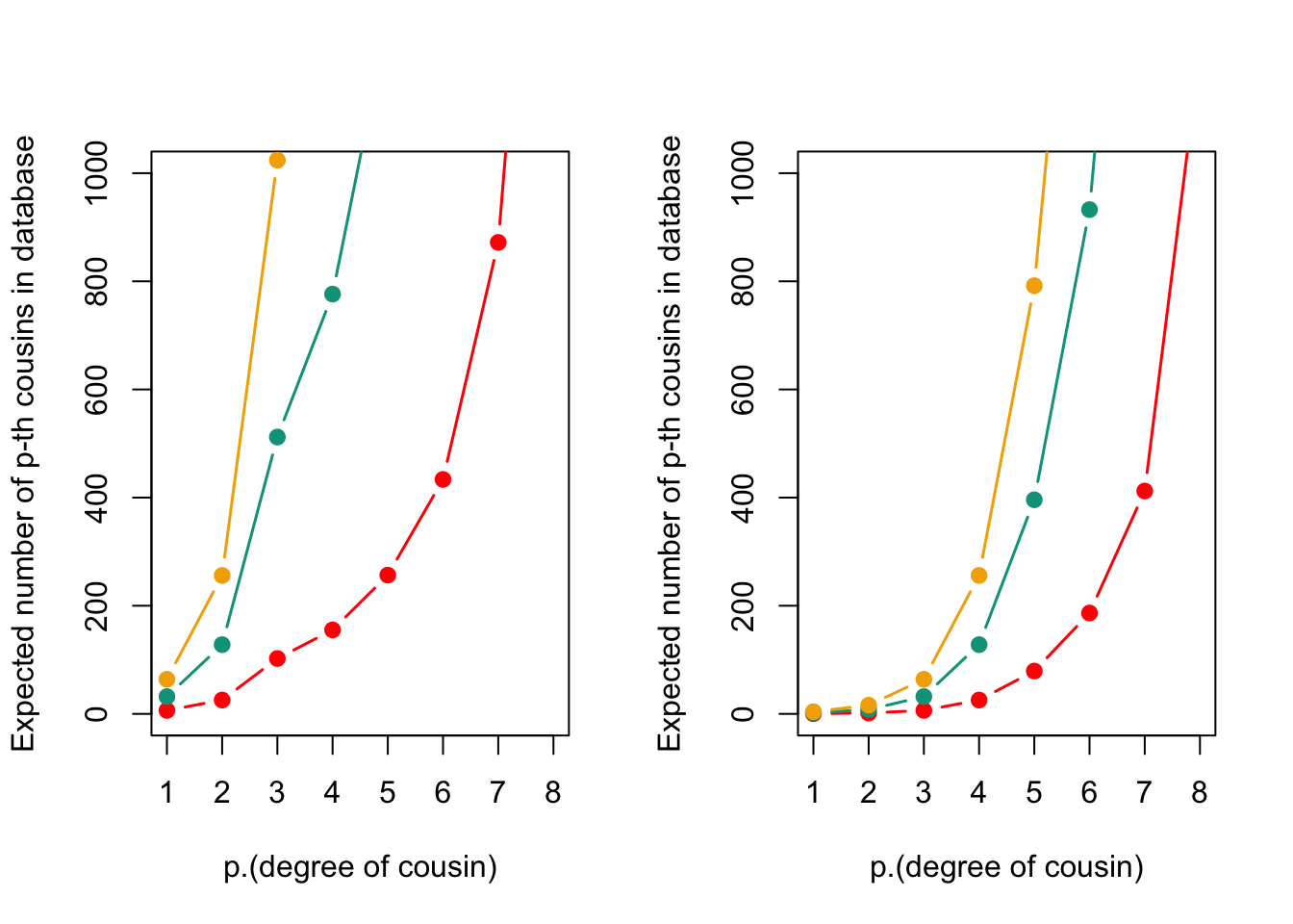

This figure the expected number of cousins for White Americans (left) and Black Americans (right) based on database sizes of 1 million, 5 million, and 10 million individuals. The expected number of cousins increases with increasing database size and degree of relatedness

Version	Author	Date
5f805fe	Tina Lasisi	2023-03-05

[[1]]
NULL

[[2]]
NULL

[[3]]
NULL

Probability of a genetically detectable cousin

Below, we calculate the expected number of shared blocks of genetic material between cousins of varying degrees of relatedness. This is important because the probability of detecting genetic material that is shared between two individuals decreases as the degree of relatedness between them decreases. The code uses a Poisson distribution assumption to estimate the probability of two cousins sharing at least one, two, or three blocks of genetic material, based on the expected number of shared blocks of genetic material calculated from previous research.

# The variable 'meiosis' represents the number of meiosis events between cousins, where 'p' is the degree of relatedness (i.e. p = 1 for first cousins, p = 2 for second cousins, etc.)
meiosis <- p + 1

## Expected number of blocks shared between cousins
# 'E.num.blocks' is the expected number of blocks of shared genetic material between cousins based on the degree of relatedness and the number of meiosis events between them. This value is calculated based on previous research and is not calculated in this code.
E.num.blocks <- 2 * (33.8 * (2 * meiosis) + 22) / (2^(2 * meiosis - 1))

## Use Poisson assumption
# 'Prob.genetic' is the probability of two cousins sharing at least one block of genetic material based on the expected number of shared blocks calculated in the previous step. The calculation uses a Poisson distribution assumption.
Prob.genetic <- 1 - exp(-E.num.blocks)

# 'prob.g.e.2.blocks' is the probability of two cousins sharing at least two blocks of genetic material based on the expected number of shared blocks calculated in the previous step. The calculation uses a Poisson distribution assumption.
prob.g.e.2.blocks <- 1 - sapply(E.num.blocks, function(expected.num) {sum(dpois(0:1, expected.num))})

# 'prob.g.e.3.blocks' is the probability of two cousins sharing at least three blocks of genetic material based on the expected number of shared blocks calculated in the previous step. The calculation uses a Poisson distribution assumption.
prob.g.e.3.blocks <- 1 - sapply(E.num.blocks, function(expected.num) {sum(dpois(0:2, expected.num))})

General

## Plot for number of shared blocks with p-th degree cousins
# Set layout of plot
layout(t(1))

# Set color palette for plot
my.cols2<-wes_palette("FantasticFox1")[3:5]

# Create a blank plot with labeled axes
plot(c(1,8),c(0,1),type="n",ylab="Probability p-th cousin \"detectable\"",xlab="p.(degree of cousin)")

# Add points for probability of detecting pth cousin with genomic blocks using colors from my.cols2
points(p,Prob.genetic,col=my.cols2[1],pch=19,type="b",lwd=2)
points(p,prob.g.e.2.blocks,col=my.cols2[2],pch=19,type="b",lwd=2)
points(p,prob.g.e.3.blocks,col=my.cols2[3],pch=19,type="b",lwd=2)

# Add a legend to the plot
legend(x="topright",legend=c("Cousins (w. >0 genomic blocks)","Cousins (w. >1 genomic blocks)","Cousins (w. >2 genomic blocks)"),col=my.cols2[1:3],lty=1)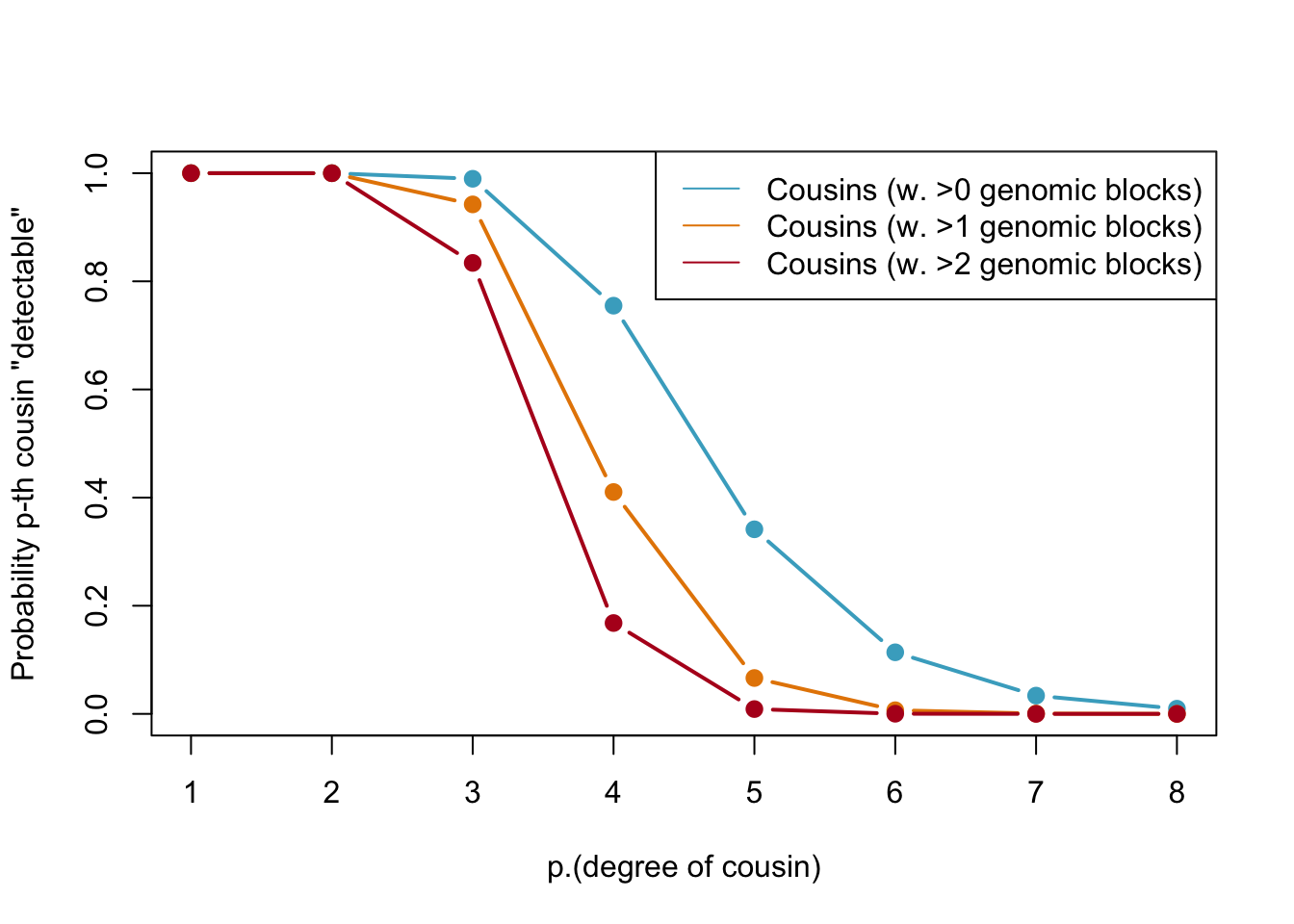

Probabilities of detecting a genetic cousin in a database based on shared genomic blocks. Blue lines represent cousins with at least one genomic block, orange dotted and red lines represent cousins with at least two and three genomic blocks, respectively. The legend specifies the type of cousin being represented by each line.

Version	Author	Date
5f805fe	Tina Lasisi	2023-03-05

Relative to database size

plt_cousins_database <- function(p, DB.sizes, N, prob.g.e.3.blocks, my.cols) {

  # Create plot
  plot(c(1, 8), c(0, 500), type = "n", ylab = "Expected number of genetic p-th cousins in database", xlab = "p. (degree of cousin)")

  # Calculate and plot expected number of genetic cousins for each database size
  sapply(1:length(DB.sizes), function(i) {
    num.cousins <- 4^(p) * DB.sizes[i] / (N / 2)
    points(p, num.cousins * prob.g.e.3.blocks, type = "b", lty = 1, col = my.cols[i])
  })

  # Create legend for plot
  my.leg <- c(c("Genetic Cousins", ">2 blocks"), c("Database size (Millions) =", format(DB.sizes / 1e6, dig = 1)))
  legend(x = "topright", legend = my.leg, col = c(NA, rep("black", 1), NA, my.cols), lty = c(NA, 1:2, rep(NA, 3)), pch = c(rep(NA, 3), rep(19, 3)))
}


layout(t(1:2))

# plt_cousins_database(p, DB.sizes, N$White, prob.g.e.3.blocks,  my.cols)
plt_cousins_database(p, DB.sizes.EUR, N$White, prob.g.e.3.blocks,  my.cols)
plt_cousins_database(p, DB.sizes.AFR, N$Black, prob.g.e.3.blocks,  my.cols)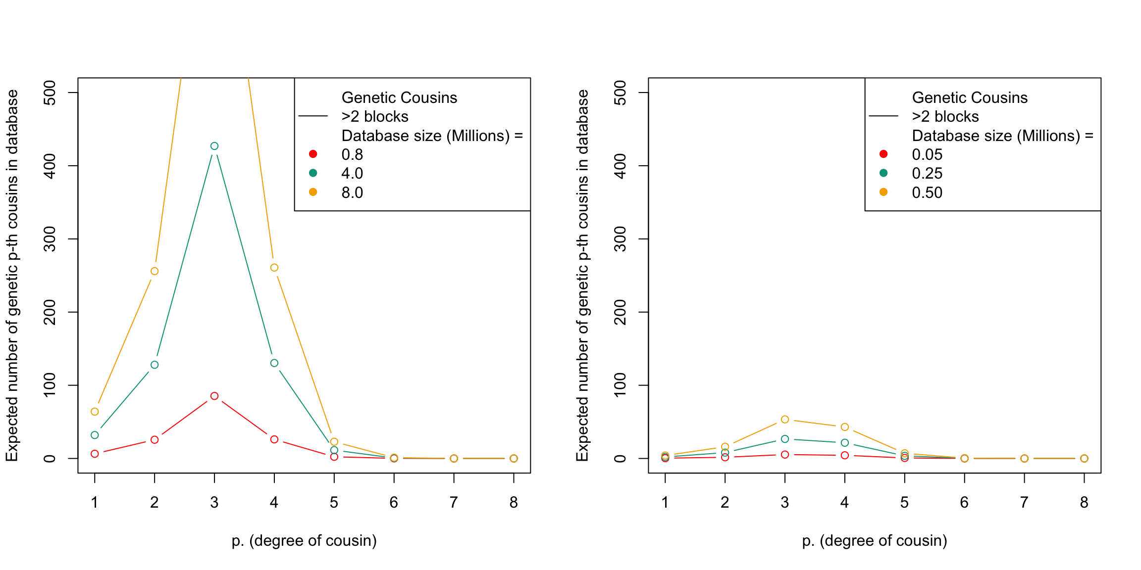

This figure shows the expected number of genetic relatives of degree p in a database of a given size. The x-axis represents the degree of relatedness

Version	Author	Date
5f805fe	Tina Lasisi	2023-03-05

sessionInfo()

R version 4.2.2 (2022-10-31)
Platform: aarch64-apple-darwin20 (64-bit)
Running under: macOS Ventura 13.0.1

Matrix products: default
BLAS:   /Library/Frameworks/R.framework/Versions/4.2-arm64/Resources/lib/libRblas.0.dylib
LAPACK: /Library/Frameworks/R.framework/Versions/4.2-arm64/Resources/lib/libRlapack.dylib

locale:
[1] en_US.UTF-8/en_US.UTF-8/en_US.UTF-8/C/en_US.UTF-8/en_US.UTF-8

attached base packages:
[1] stats     graphics  grDevices utils     datasets  methods   base     

other attached packages:
 [1] forcats_0.5.2     stringr_1.5.0     dplyr_1.0.10      purrr_0.3.5      
 [5] readr_2.1.3       tidyr_1.2.1       tibble_3.1.8      ggplot2_3.4.0    
 [9] tidyverse_1.3.2   wesanderson_0.3.6 workflowr_1.7.0  

loaded via a namespace (and not attached):
 [1] Rcpp_1.0.9          lubridate_1.9.0     getPass_0.2-2      
 [4] ps_1.7.2            assertthat_0.2.1    rprojroot_2.0.3    
 [7] digest_0.6.30       utf8_1.2.2          R6_2.5.1           
[10] cellranger_1.1.0    backports_1.4.1     reprex_2.0.2       
[13] evaluate_0.18       highr_0.9           httr_1.4.4         
[16] pillar_1.8.1        rlang_1.0.6         readxl_1.4.1       
[19] googlesheets4_1.0.1 rstudioapi_0.14     whisker_0.4        
[22] callr_3.7.3         jquerylib_0.1.4     rmarkdown_2.18     
[25] googledrive_2.0.0   munsell_0.5.0       broom_1.0.1        
[28] modelr_0.1.10       compiler_4.2.2      httpuv_1.6.6       
[31] xfun_0.35           pkgconfig_2.0.3     htmltools_0.5.3    
[34] tidyselect_1.2.0    fansi_1.0.3         crayon_1.5.2       
[37] withr_2.5.0         tzdb_0.3.0          dbplyr_2.2.1       
[40] later_1.3.0         grid_4.2.2          jsonlite_1.8.3     
[43] gtable_0.3.1        lifecycle_1.0.3     DBI_1.1.3          
[46] git2r_0.30.1        magrittr_2.0.3      scales_1.2.1       
[49] cli_3.4.1           stringi_1.7.8       cachem_1.0.6       
[52] fs_1.5.2            promises_1.2.0.1    xml2_1.3.3         
[55] bslib_0.4.1         ellipsis_0.3.2      generics_0.1.3     
[58] vctrs_0.5.1         tools_4.2.2         glue_1.6.2         
[61] hms_1.1.2           processx_3.8.0      fastmap_1.1.0      
[64] yaml_2.3.6          timechange_0.1.1    colorspace_2.0-3   
[67] gargle_1.2.1        rvest_1.0.3         knitr_1.41         
[70] haven_2.5.1         sass_0.4.4