Short Range Familial Search

Last updated: 2024-01-22

Checks: 7 0

Knit directory: PODFRIDGE/

This reproducible R Markdown analysis was created with workflowr (version 1.7.1). The Checks tab describes the reproducibility checks that were applied when the results were created. The Past versions tab lists the development history.

R Markdown file: up-to-date

Great! Since the R Markdown file has been committed to the Git repository, you know the exact version of the code that produced these results.

Environment: empty

Great job! The global environment was empty. Objects defined in the global environment can affect the analysis in your R Markdown file in unknown ways. For reproduciblity it’s best to always run the code in an empty environment.

Seed: set.seed(20230302)

The command set.seed(20230302) was run prior to running the code in the R Markdown file. Setting a seed ensures that any results that rely on randomness, e.g. subsampling or permutations, are reproducible.

Session information: recorded

Great job! Recording the operating system, R version, and package versions is critical for reproducibility.

Cache: none

Nice! There were no cached chunks for this analysis, so you can be confident that you successfully produced the results during this run.

File paths: relative

Great job! Using relative paths to the files within your workflowr project makes it easier to run your code on other machines.

Repository version: 1f3a662

Great! You are using Git for version control. Tracking code development and connecting the code version to the results is critical for reproducibility.

The results in this page were generated with repository version 1f3a662. See the Past versions tab to see a history of the changes made to the R Markdown and HTML files.

Note that you need to be careful to ensure that all relevant files for the analysis have been committed to Git prior to generating the results (you can use wflow_publish or wflow_git_commit). workflowr only checks the R Markdown file, but you know if there are other scripts or data files that it depends on. Below is the status of the Git repository when the results were generated:


Ignored files:
    Ignored:    .DS_Store
    Ignored:    .Rhistory
    Ignored:    .Rproj.user/

Unstaged changes:
    Modified:   analysis/_site.yml

Note that any generated files, e.g. HTML, png, CSS, etc., are not included in this status report because it is ok for generated content to have uncommitted changes.

These are the previous versions of the repository in which changes were made to the R Markdown (analysis/shortrange.Rmd) and HTML (docs/shortrange.html) files. If you’ve configured a remote Git repository (see ?wflow_git_remote), click on the hyperlinks in the table below to view the files as they were in that past version.

File	Version	Author	Date	Message
html	8a464dc	Tina Lasisi	2024-01-18	Updated shortrange links + re-built website
Rmd	d959019	Tina Lasisi	2023-05-31	Add STR.Rmd
Rmd	8b2d06a	Tina Lasisi	2023-05-23	Remove excess data + comment code
Rmd	345b867	Tina Lasisi	2023-05-22	Update shortrange.Rmd
Rmd	ab788f7	Tina Lasisi	2023-05-22	Upload short range material
html	ab788f7	Tina Lasisi	2023-05-22	Upload short range material

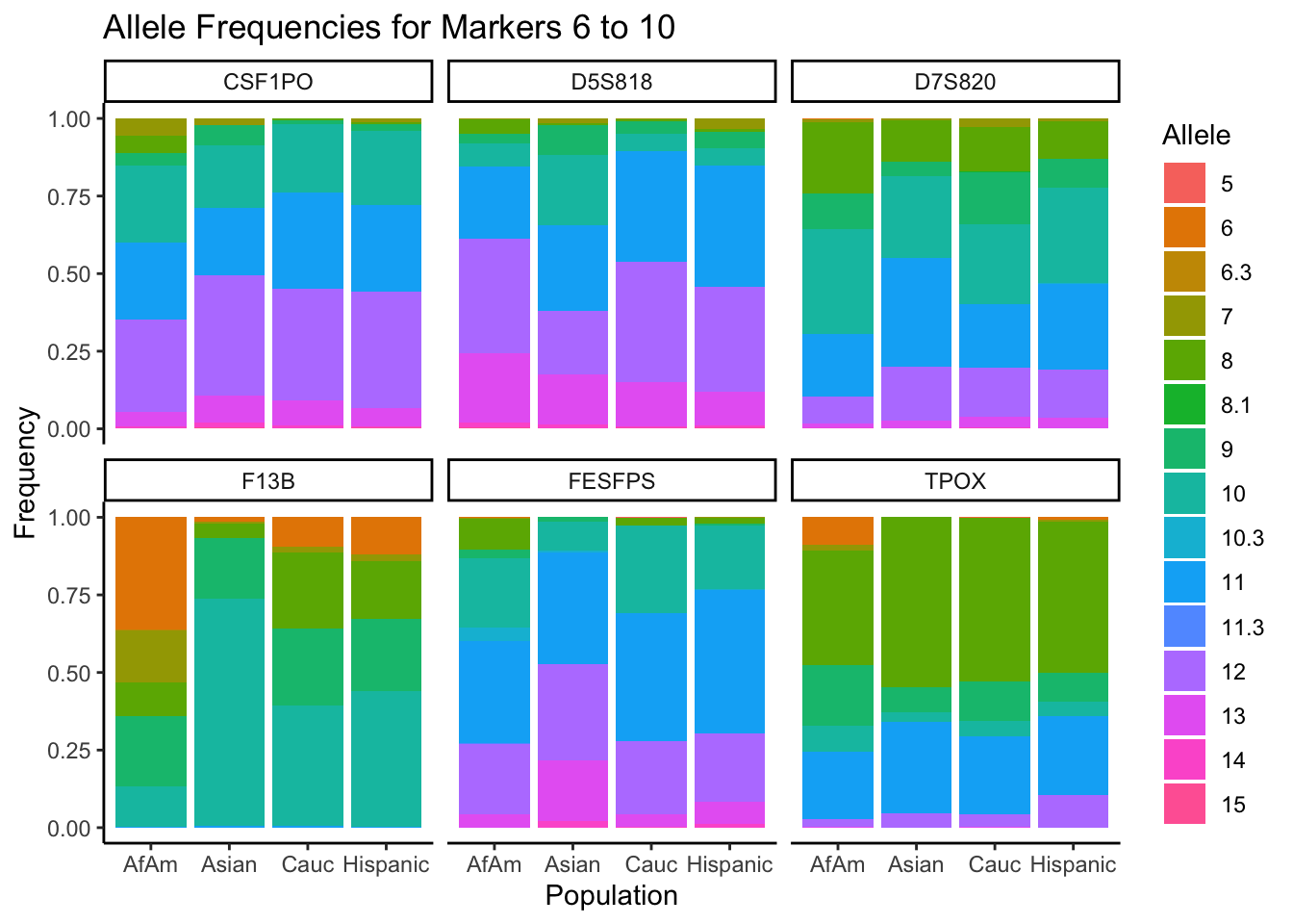
CODIS marker allele frequencies

Frequencies and raw genotypes for different populations were found here and refer to Steffen, C.R., Coble, M.D., Gettings, K.B., Vallone, P.M. (2017) Corrigendum to ‘U.S. Population Data for 29 Autosomal STR Loci’ [Forensic Sci. Int. Genet. 7 (2013) e82-e83]. Forensic Sci. Int. Genet. 31, e36–e40. The US core CODIS markers are a subset of the 29 described here.

Load CODIS allele frequencies

CODIS allele frequencies were found through NIST STR base and specifically downloaded from the supplementary materials of Steffen et al 2017. These are 1036 unrelated individuals from the U.S. population.

# Define the file paths
file_paths <- list.files(path = "data", pattern = "1036_.*\\.csv", full.names = TRUE)

# Create a list of data frames
df_list <- lapply(file_paths, function(path) {
  read_csv(path, col_types = cols(
    marker = col_character(),
    allele = col_double(),
    frequency = col_double(),
    population = col_character()
  ))
})

# Bind all data frames into one
df <- bind_rows(df_list)

# Find unique markers and split them into chunks of 5
unique_markers <- unique(df$marker)
marker_chunks <- split(unique_markers, ceiling(seq_along(unique_markers)/5))

# Loop through the chunks and create a plot for each chunk
for(i in seq_along(marker_chunks)) {
  df_chunk <- df %>% filter(marker %in% marker_chunks[[i]])
  
  p <- ggplot(df_chunk, aes(x = allele, y = frequency, fill = population)) +
    geom_col(position = "dodge", width = 0.7) +
    facet_grid(population ~ marker) +
    # scale_x_continuous(breaks = seq(2.2, 43.2, by = 1)) +
    labs(x = "Allele", y = "Frequency",
         title = paste("Allele Frequencies for Markers", i*5-4, "to", min(i*5, length(unique_markers))),
         caption = "Source: CSV data") +
    theme_bw()

  print(p)
}

Warning: `position_dodge()` requires non-overlapping x intervals
`position_dodge()` requires non-overlapping x intervals
`position_dodge()` requires non-overlapping x intervals
`position_dodge()` requires non-overlapping x intervals
`position_dodge()` requires non-overlapping x intervals
`position_dodge()` requires non-overlapping x intervals
`position_dodge()` requires non-overlapping x intervals
`position_dodge()` requires non-overlapping x intervals
`position_dodge()` requires non-overlapping x intervals
`position_dodge()` requires non-overlapping x intervals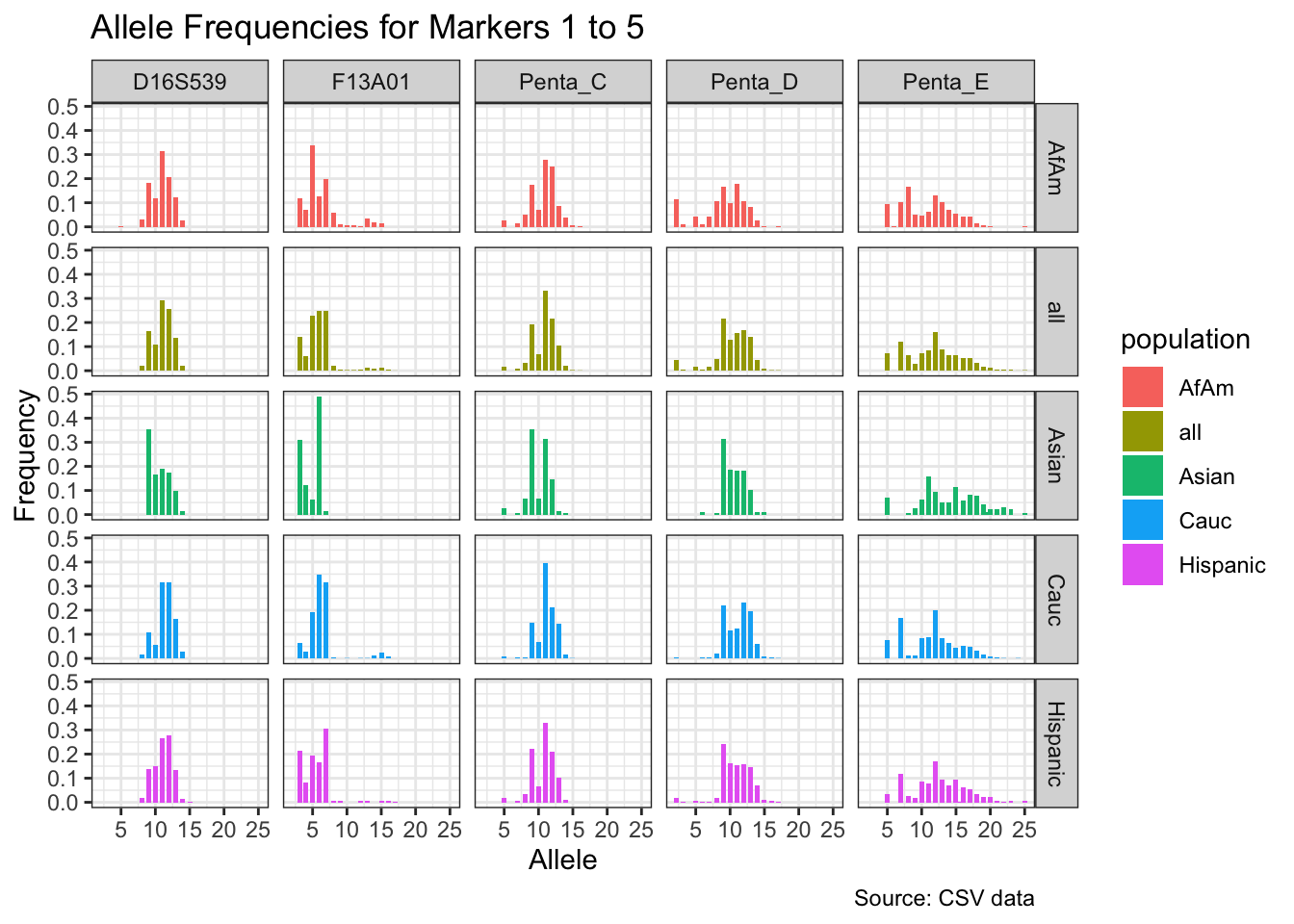

Version	Author	Date
8a464dc	Tina Lasisi	2024-01-18

Warning: `position_dodge()` requires non-overlapping x intervals
`position_dodge()` requires non-overlapping x intervals
`position_dodge()` requires non-overlapping x intervals
`position_dodge()` requires non-overlapping x intervals
`position_dodge()` requires non-overlapping x intervals
`position_dodge()` requires non-overlapping x intervals
`position_dodge()` requires non-overlapping x intervals
`position_dodge()` requires non-overlapping x intervals
`position_dodge()` requires non-overlapping x intervals
`position_dodge()` requires non-overlapping x intervals
`position_dodge()` requires non-overlapping x intervals
`position_dodge()` requires non-overlapping x intervals
`position_dodge()` requires non-overlapping x intervals
`position_dodge()` requires non-overlapping x intervals

Version	Author	Date
8a464dc	Tina Lasisi	2024-01-18

Warning: `position_dodge()` requires non-overlapping x intervals
`position_dodge()` requires non-overlapping x intervals
`position_dodge()` requires non-overlapping x intervals
`position_dodge()` requires non-overlapping x intervals
`position_dodge()` requires non-overlapping x intervals

Version	Author	Date
8a464dc	Tina Lasisi	2024-01-18

Warning: `position_dodge()` requires non-overlapping x intervals
`position_dodge()` requires non-overlapping x intervals
`position_dodge()` requires non-overlapping x intervals
`position_dodge()` requires non-overlapping x intervals
`position_dodge()` requires non-overlapping x intervals
`position_dodge()` requires non-overlapping x intervals
`position_dodge()` requires non-overlapping x intervals
`position_dodge()` requires non-overlapping x intervals
`position_dodge()` requires non-overlapping x intervals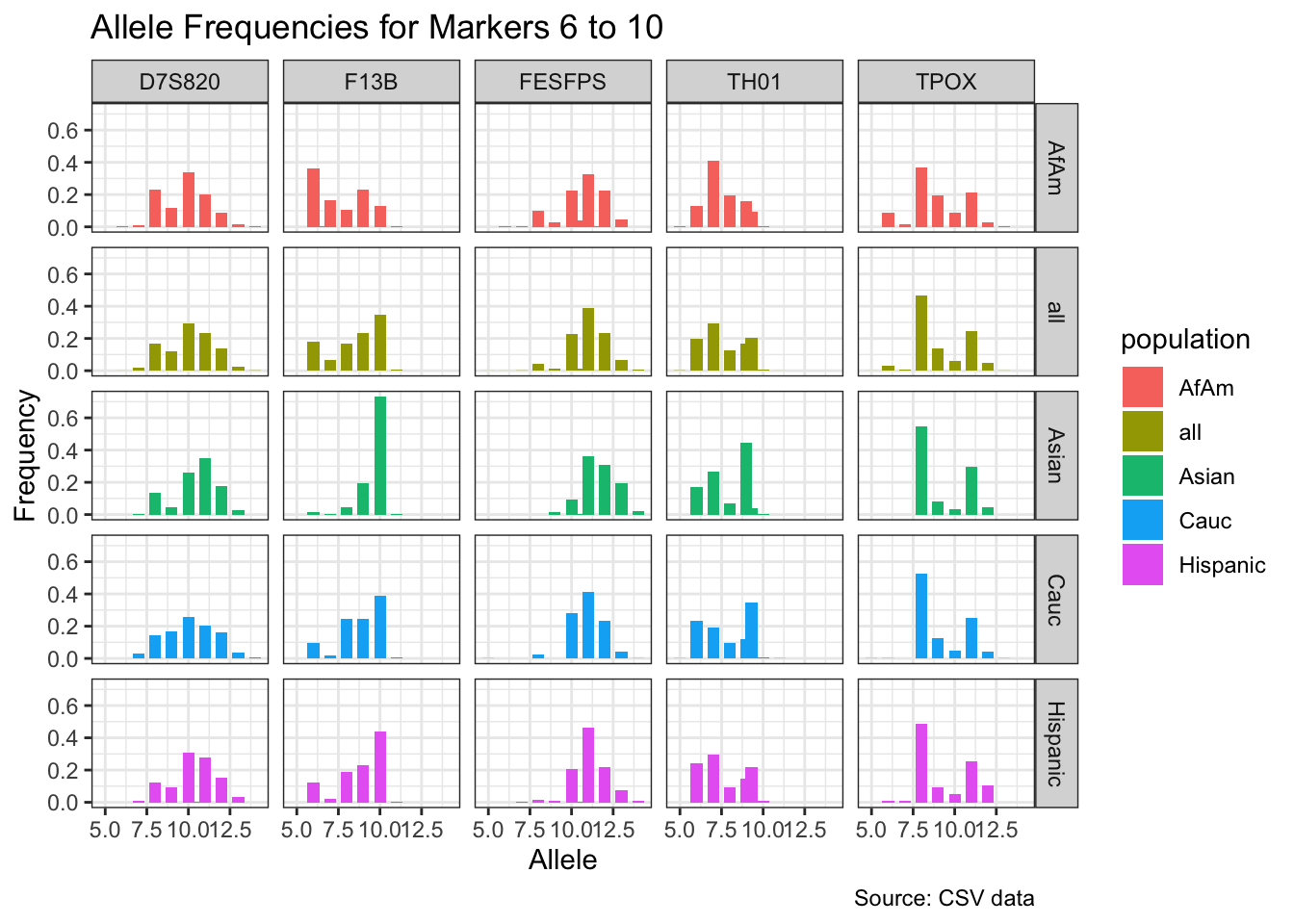

Version	Author	Date
8a464dc	Tina Lasisi	2024-01-18

Warning: `position_dodge()` requires non-overlapping x intervals
`position_dodge()` requires non-overlapping x intervals
`position_dodge()` requires non-overlapping x intervals
`position_dodge()` requires non-overlapping x intervals
`position_dodge()` requires non-overlapping x intervals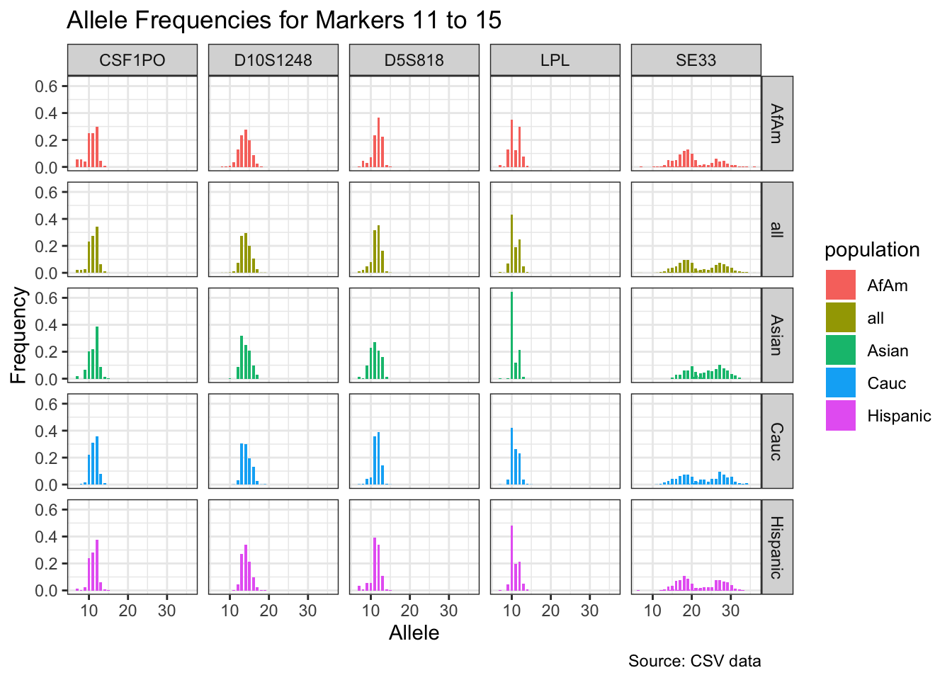
`position_dodge()` requires non-overlapping x intervals
`position_dodge()` requires non-overlapping x intervals
`position_dodge()` requires non-overlapping x intervals
`position_dodge()` requires non-overlapping x intervals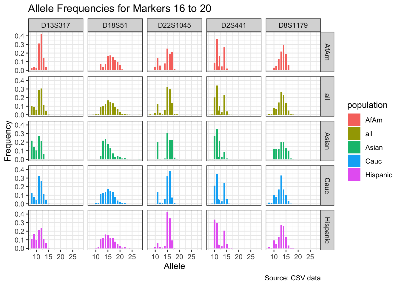
`position_dodge()` requires non-overlapping x intervals
`position_dodge()` requires non-overlapping x intervals
`position_dodge()` requires non-overlapping x intervals
`position_dodge()` requires non-overlapping x intervals
`position_dodge()` requires non-overlapping x intervals
`position_dodge()` requires non-overlapping x intervals
`position_dodge()` requires non-overlapping x intervals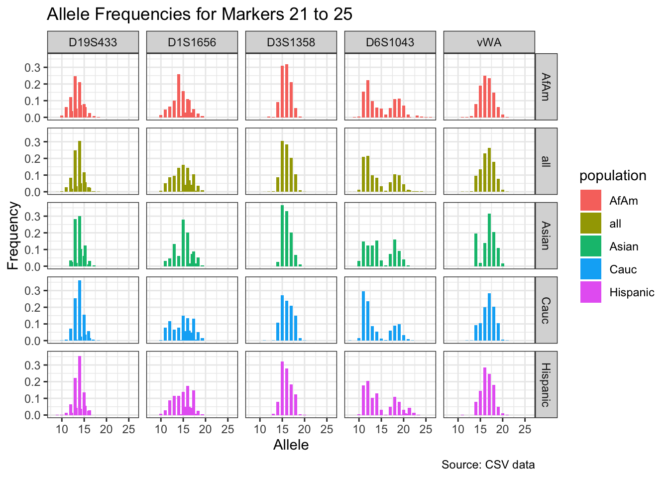

Version	Author	Date
8a464dc	Tina Lasisi	2024-01-18

Warning: `position_dodge()` requires non-overlapping x intervals
`position_dodge()` requires non-overlapping x intervals
`position_dodge()` requires non-overlapping x intervals
`position_dodge()` requires non-overlapping x intervals
`position_dodge()` requires non-overlapping x intervals
`position_dodge()` requires non-overlapping x intervals
`position_dodge()` requires non-overlapping x intervals
`position_dodge()` requires non-overlapping x intervals
`position_dodge()` requires non-overlapping x intervals
`position_dodge()` requires non-overlapping x intervals
`position_dodge()` requires non-overlapping x intervals
`position_dodge()` requires non-overlapping x intervals
`position_dodge()` requires non-overlapping x intervals
`position_dodge()` requires non-overlapping x intervals
`position_dodge()` requires non-overlapping x intervals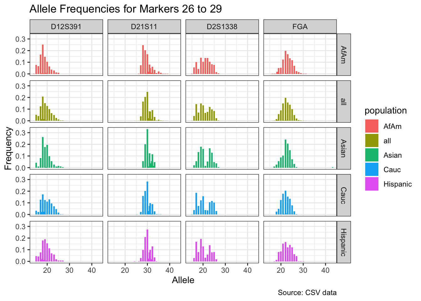

Version	Author	Date
8a464dc	Tina Lasisi	2024-01-18

df %>%
  group_by(population) %>%
  filter(population != "all") %>%
  ggplot(aes(x = marker, y = allele, fill = population)) +
  geom_boxplot() +
  labs(x = "Marker", y = "Allele",
       title = "Range of Alleles Across Different Markers (Grouped by Population)") +
    theme(axis.text.x = element_text(angle = 45, hjust = 1))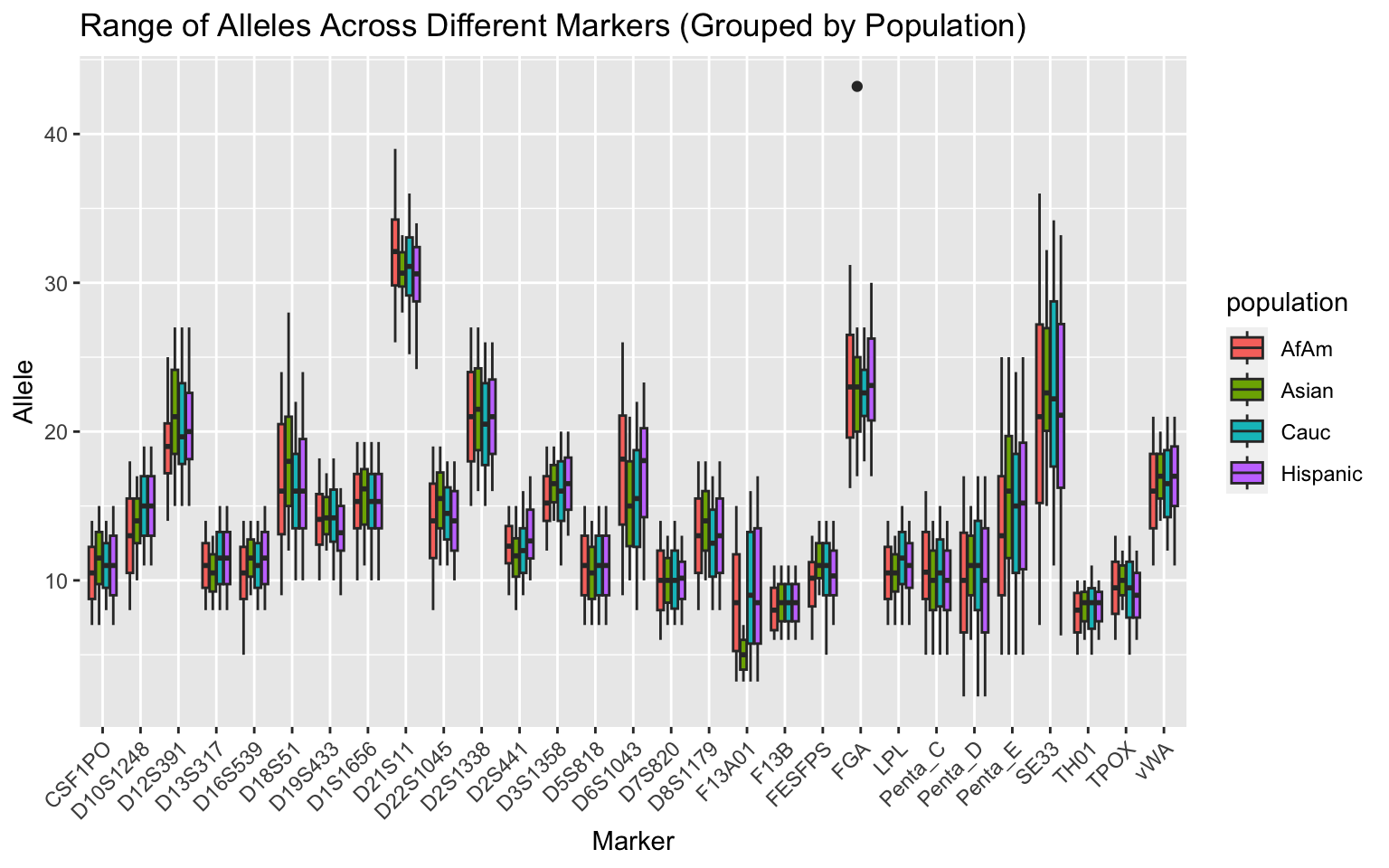

Version	Author	Date
8a464dc	Tina Lasisi	2024-01-18

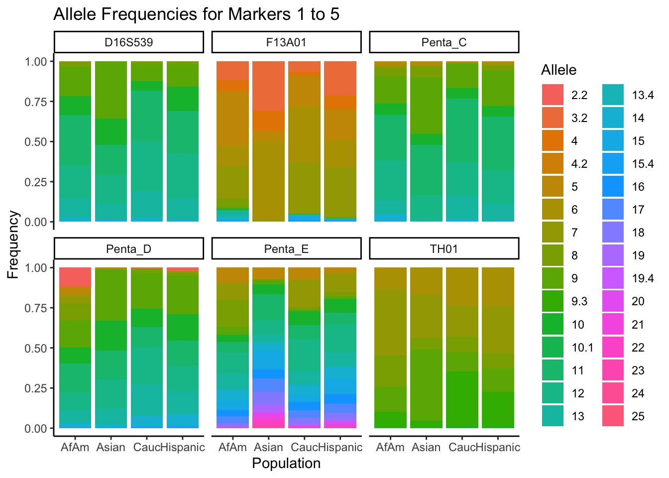
# Filter out the "all" population
df_filtered <- df %>% filter(population != "all")

# Get the unique markers and split them into chunks of 5
unique_markers <- unique(df_filtered$marker)
marker_chunks <- split(unique_markers, ceiling(seq_along(unique_markers)/6))

# Loop through the chunks
for(i in seq_along(marker_chunks)) {
  
  # Subset the data for the current chunk of markers
  df_chunk <- df_filtered %>% filter(marker %in% marker_chunks[[i]])
  
  # Convert the allele variable to a factor
  df_chunk$allele <- as.factor(df_chunk$allele)
  
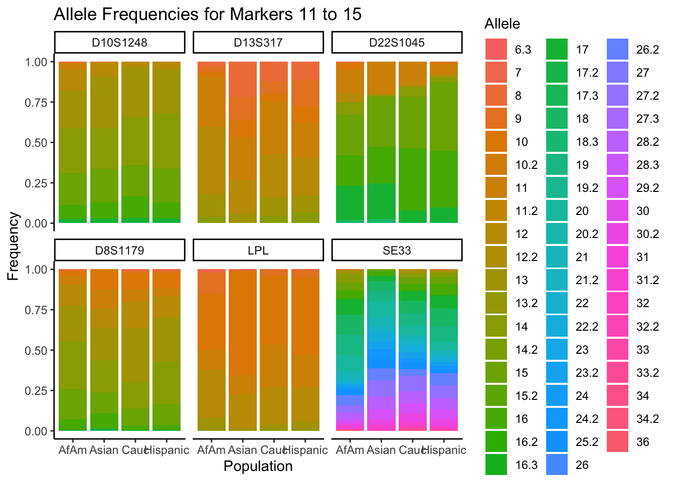
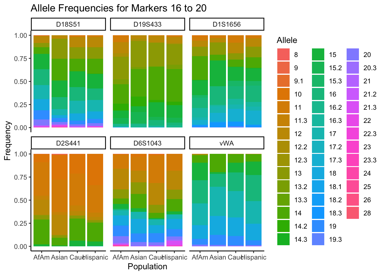
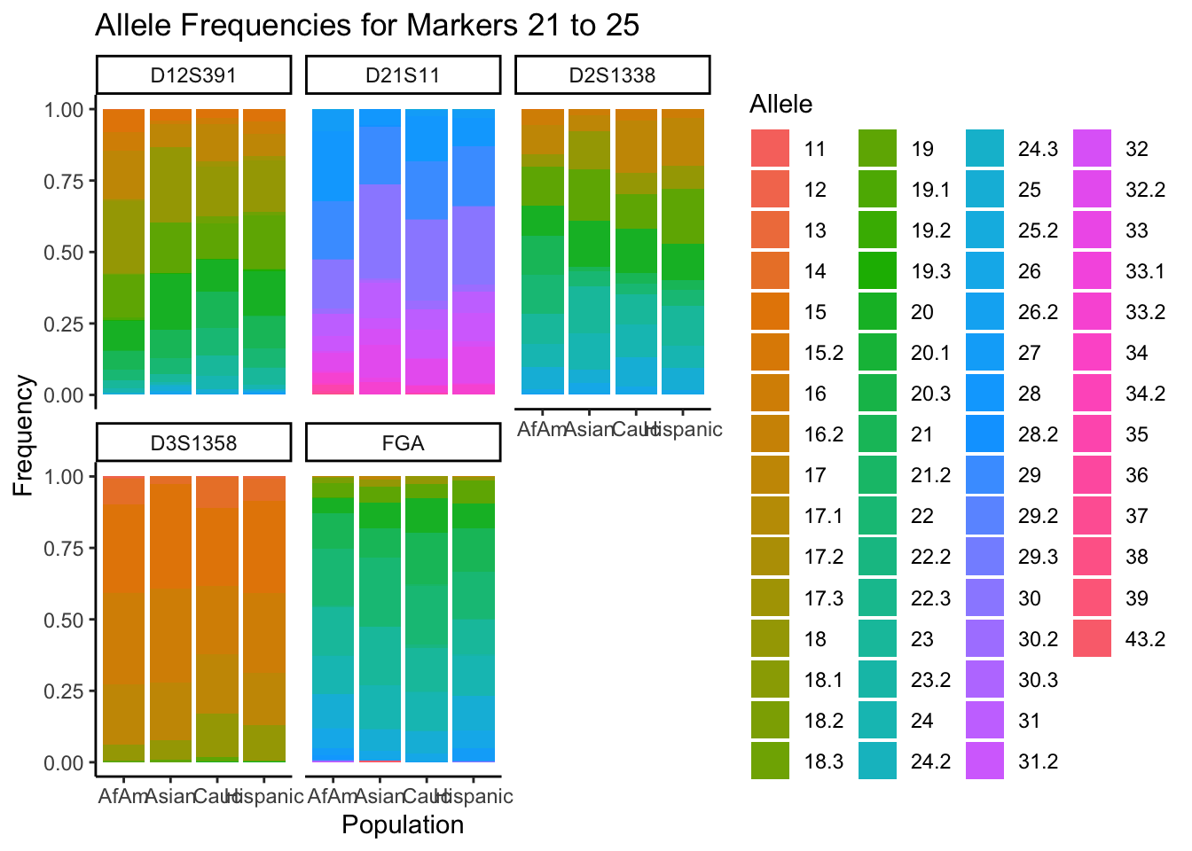
  # Create the plot
  p <- ggplot(df_chunk, aes(x = population, y = frequency, fill = allele)) +
    geom_bar(stat = "identity") +
    facet_wrap(~ marker) +
    labs(x = "Population", y = "Frequency", fill = "Allele",
         title = paste("Allele Frequencies for Markers", i*5-4, "to", min(i*5, length(unique_markers)))) +
    theme_classic()  # Apply theme_classic()
  
  # Print the plot
  print(p)
}

Version	Author	Date
8a464dc	Tina Lasisi	2024-01-18
ab788f7	Tina Lasisi	2023-05-22

Version	Author	Date
8a464dc	Tina Lasisi	2024-01-18
ab788f7	Tina Lasisi	2023-05-22

Version	Author	Date
8a464dc	Tina Lasisi	2024-01-18
ab788f7	Tina Lasisi	2023-05-22

Version	Author	Date
8a464dc	Tina Lasisi	2024-01-18
ab788f7	Tina Lasisi	2023-05-22

Version	Author	Date
8a464dc	Tina Lasisi	2024-01-18
ab788f7	Tina Lasisi	2023-05-22

summary_df <- df %>%
  group_by(marker, population) %>%
  summarise(num_alleles = n_distinct(allele))

`summarise()` has grouped output by 'marker'. You can override using the
`.groups` argument.

summary_df

# A tibble: 145 × 3
# Groups:   marker [29]
   marker   population num_alleles
   <chr>    <chr>            <int>
 1 CSF1PO   AfAm                 8
 2 CSF1PO   Asian                8
 3 CSF1PO   Cauc                 7
 4 CSF1PO   Hispanic             9
 5 CSF1PO   all                  9
 6 D10S1248 AfAm                11
 7 D10S1248 Asian                7
 8 D10S1248 Cauc                 9
 9 D10S1248 Hispanic             9
10 D10S1248 all                 12
# ℹ 135 more rows

summary_df <- df %>%
  group_by(marker, population) %>%
  summarise(num_alleles = n_distinct(allele))

`summarise()` has grouped output by 'marker'. You can override using the
`.groups` argument.

summary_pivot <- summary_df %>%
  pivot_wider(names_from = population, values_from = num_alleles)

summary_pivot

# A tibble: 29 × 6
# Groups:   marker [29]
   marker    AfAm Asian  Cauc Hispanic   all
   <chr>    <int> <int> <int>    <int> <int>
 1 CSF1PO       8     8     7        9     9
 2 D10S1248    11     7     9        9    12
 3 D12S391     19    15    16       19    24
 4 D13S317      7     6     8        8     8
 5 D16S539      8     6     7        8     9
 6 D18S51      19    13    15       15    22
 7 D19S433     14    11    15       13    16
 8 D1S1656     15    12    15       15    15
 9 D21S11      20    12    16       16    27
10 D22S1045    11     8     8        9    11
# ℹ 19 more rows

Simulating genotypes

One marker at a time

# Function to simulate genotypes for a pair of individuals
simulate_genotypes <- function(allele_frequencies, relationship_type) {
  # Draw two alleles for the first individual from the population allele frequencies
  individual1 <- sample(names(allele_frequencies), size = 2, replace = TRUE, prob = allele_frequencies)
  
  # Define the probabilities of sharing 0, 1, or 2 IBD alleles for each relationship type
  relationship_probs <- list(
    'parent_child' = c(0, 1, 0), # In a parent-child relationship, always 1 allele is shared
    'full_siblings' = c(1/4, 1/2, 1/4), # For full siblings, the probabilities are 1/4 for sharing 0, 1/2 for sharing 1, and 1/4 for sharing 2 alleles
    'half_siblings' = c(1/2, 1/2, 0), # For half siblings, the probabilities are 1/2 for sharing 0 and 1/2 for sharing 1 allele
    'cousins' = c(7/8, 1/8, 0), # For cousins, the probabilities are 7/8 for sharing 0 and 1/8 for sharing 1 allele
    'second_cousins' = c(15/16, 1/16, 0), # For second cousins, the probabilities are 15/16 for sharing 0 and 1/16 for sharing 1 allele
    'unrelated' = c(1, 0, 0) # For unrelated individuals, they always share 0 alleles
  )
  
  # Get the probabilities of sharing alleles for the specific relationship type
  prob_shared_alleles <- relationship_probs[[relationship_type]]
  
  # Draw the number of shared alleles based on these probabilities
  num_shared_alleles <- sample(c(0, 1, 2), size = 1, prob = prob_shared_alleles)
  
  # Construct the genotype of the second individual by sampling the shared alleles from the first individual 
  # and the rest from the population allele frequencies
  individual2 <- c(sample(individual1, size = num_shared_alleles), sample(names(allele_frequencies), size = 2 - num_shared_alleles, replace = TRUE, prob = allele_frequencies))
  
  # Return the genotypes of the two individuals and the number of shared alleles
  return(list(individual1 = individual1, individual2 = individual2, num_shared_alleles = num_shared_alleles))
}

# Function to calculate the index of relatedness
calculate_relatedness <- function(simulated_genotypes, allele_frequencies) {
  # Calculate the number of alleles that the two individuals share
  num_shared_alleles <- sum(simulated_genotypes$individual1 %in% simulated_genotypes$individual2)
  
  # Calculate the index of relatedness as the number of shared alleles divided by the sum of the inverse of allele frequencies 
  # of the alleles in the genotypes of both individuals. This gives a higher weight to rare alleles.
  relatedness <- num_shared_alleles / (sum(1 / allele_frequencies[simulated_genotypes$individual1]) + sum(1 / allele_frequencies[simulated_genotypes$individual2]))
  
    # Return the index of relatedness and the number of shared alleles
  return(list(relatedness = relatedness, num_shared_alleles = simulated_genotypes$num_shared_alleles))
}

# Function to simulate genotypes and calculate relatedness for different relationships
simulate_relatedness <- function(df, marker, population, relationship_type) {
  # Filter the data frame to get the allele frequencies for the specific marker and population
  allele_frequencies <- df %>%
    filter(marker == marker, population == population) %>%
    pull(frequency) %>%
    setNames(df$allele)
  
  # Simulate the genotypes for the pair of individuals using these allele frequencies and the specific relationship type
  simulated_genotypes <- simulate_genotypes(allele_frequencies, relationship_type)
  
  # Calculate the relatedness index based on these simulated genotypes and the allele frequencies
  relatedness_data <- calculate_relatedness(simulated_genotypes, allele_frequencies)
  
  # Return the marker, population, relationship type, and the calculated relatedness data
  return(c(list(marker = marker, population = population, relationship_type = relationship_type), relatedness_data))
}

# Example usage
simulate_relatedness(df, marker = "F13A01", population = "Asian", relationship_type = "full_siblings")

$marker
[1] "F13A01"

$population
[1] "Asian"

$relationship_type
[1] "full_siblings"

$relatedness
[1] 0

$num_shared_alleles
[1] 0

simulate_all_relationships <- function(df, num_simulations) {
  # Define the list of relationship types
  relationship_types <- c('parent_child', 'full_siblings', 'half_siblings', 'cousins', 'second_cousins', 'unrelated')
  
  # Initialize an empty list to store results
  results <- list()
  
  # Iterate over all combinations of markers, populations, and relationship types
  for (marker in unique(df$marker)) {
    for (population in unique(df$population)) {
      for (relationship_type in relationship_types) {
        for (i in 1:num_simulations) {
          # Simulate relatedness and add the result to the list
          results[[length(results) + 1]] <- simulate_relatedness(df, marker, population, relationship_type)
        }
      }
    }
  }
  
  # Convert the list of results to a dataframe
  results_df <- do.call(rbind, lapply(results, function(x) as.data.frame(t(unlist(x)))))
  
  return(results_df)
}

# Usage:
# df <- # Your dataframe here
results_df <- simulate_all_relationships(df, num_simulations = 10)

Visualization

# Function to capitalize the first letter of a string
ucfirst <- function(s) {
  paste(toupper(substring(s, 1,1)), substring(s, 2), sep = "")
}

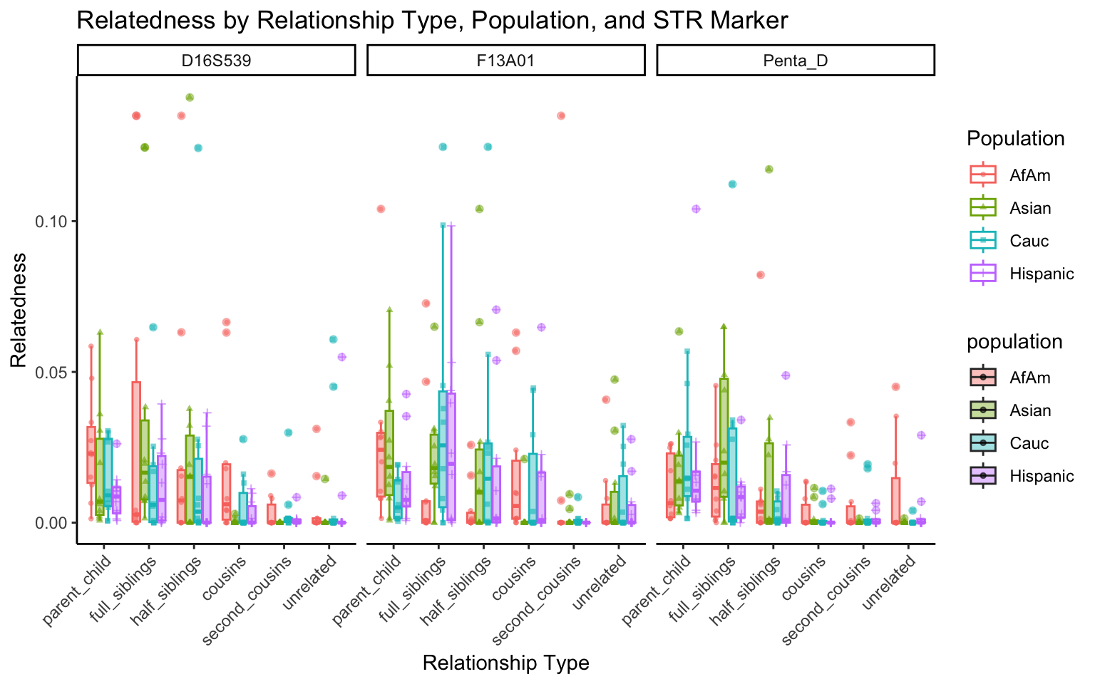
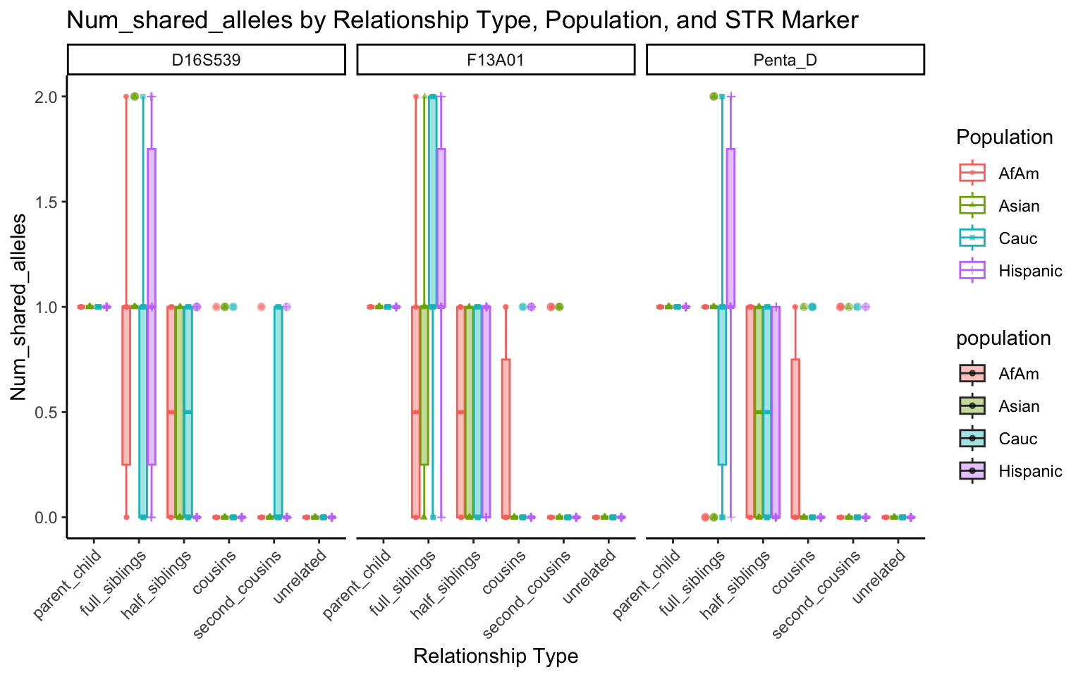
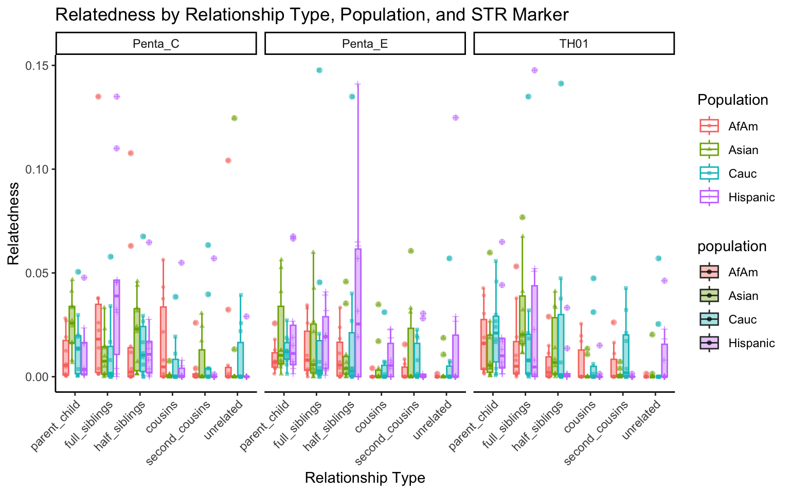
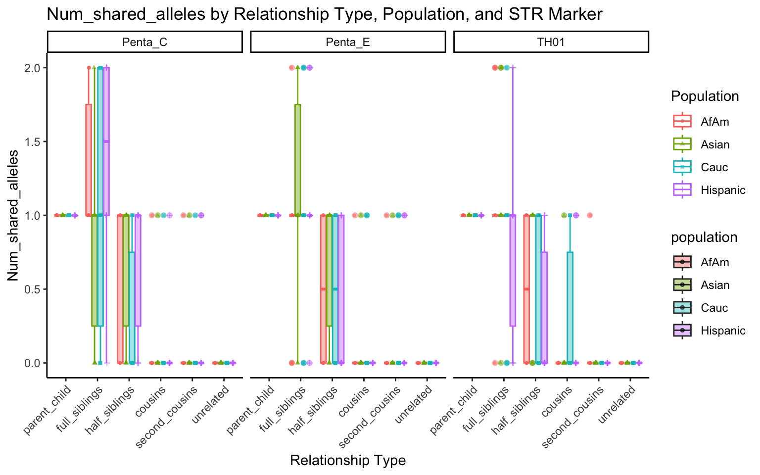
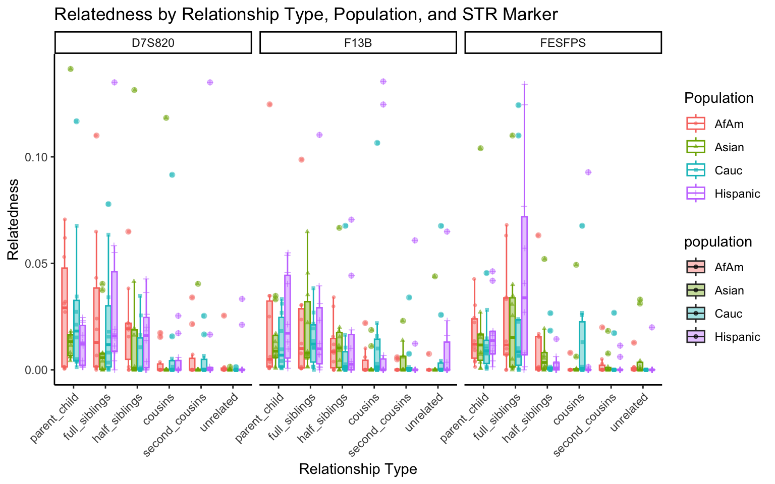
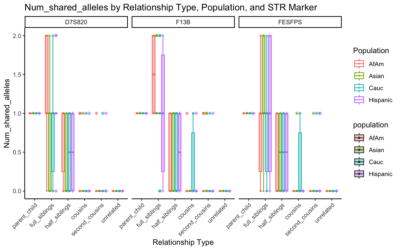
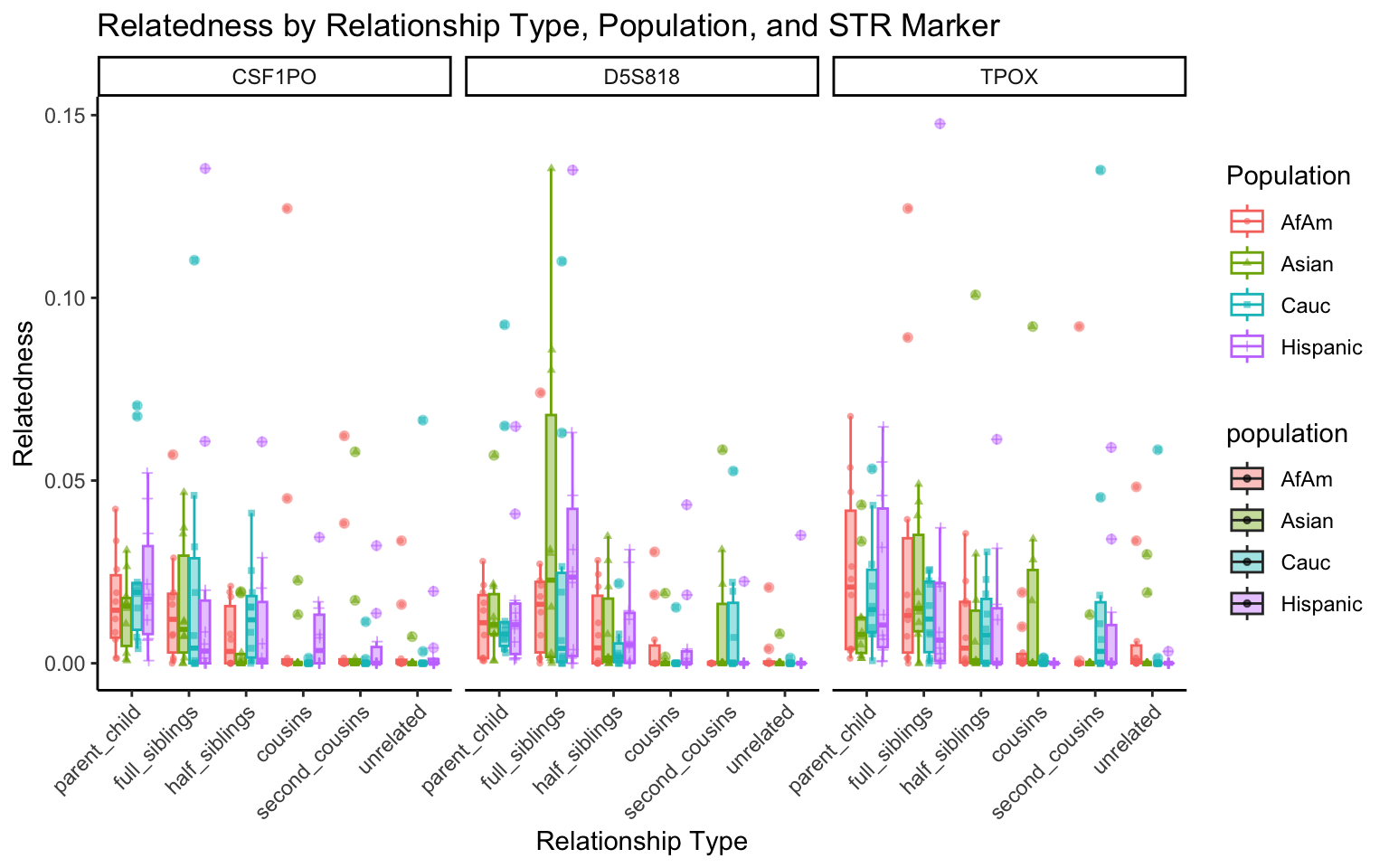
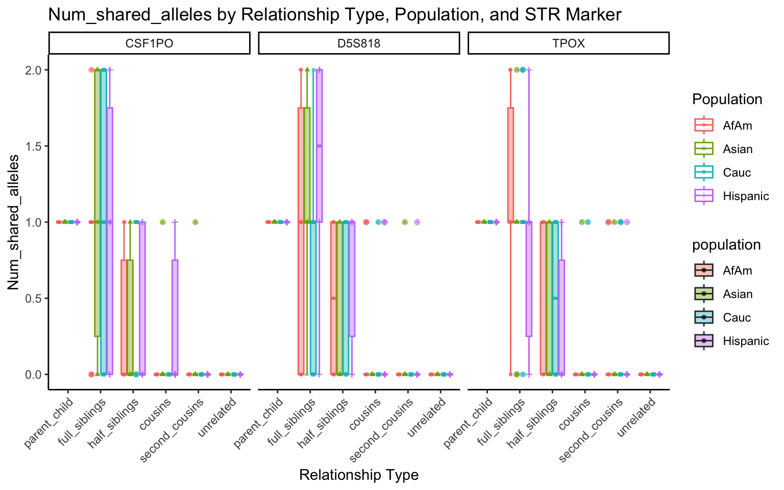
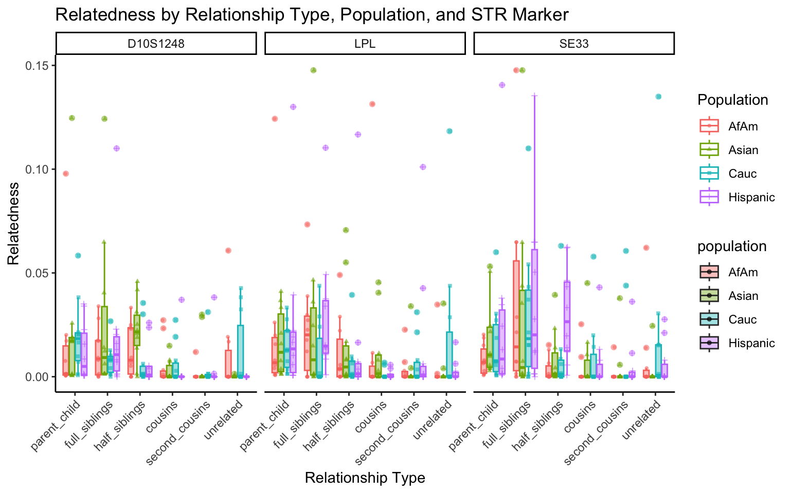
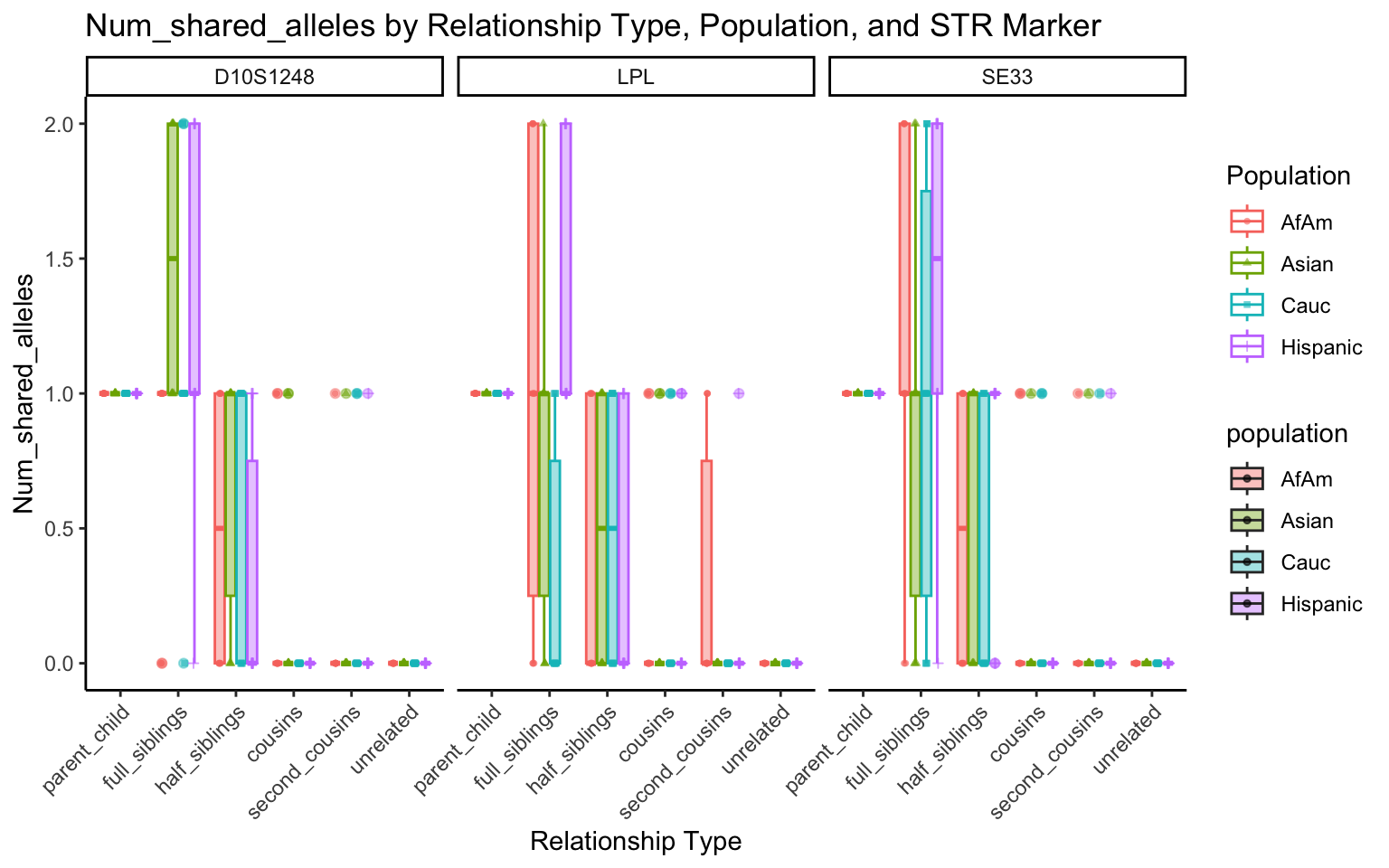
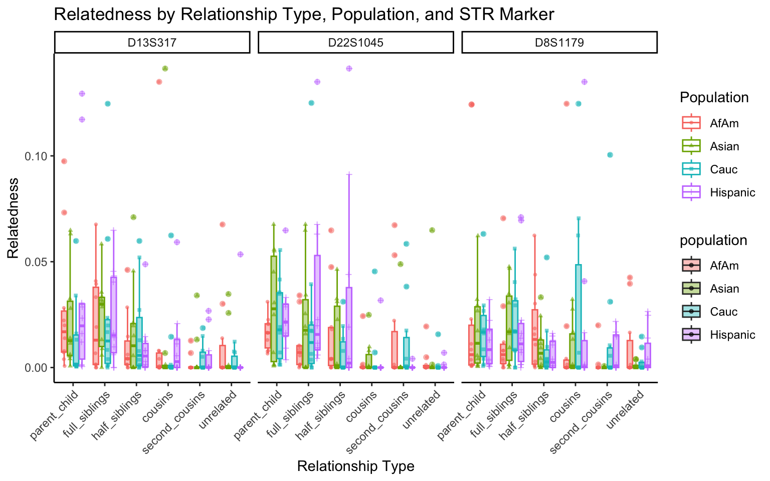
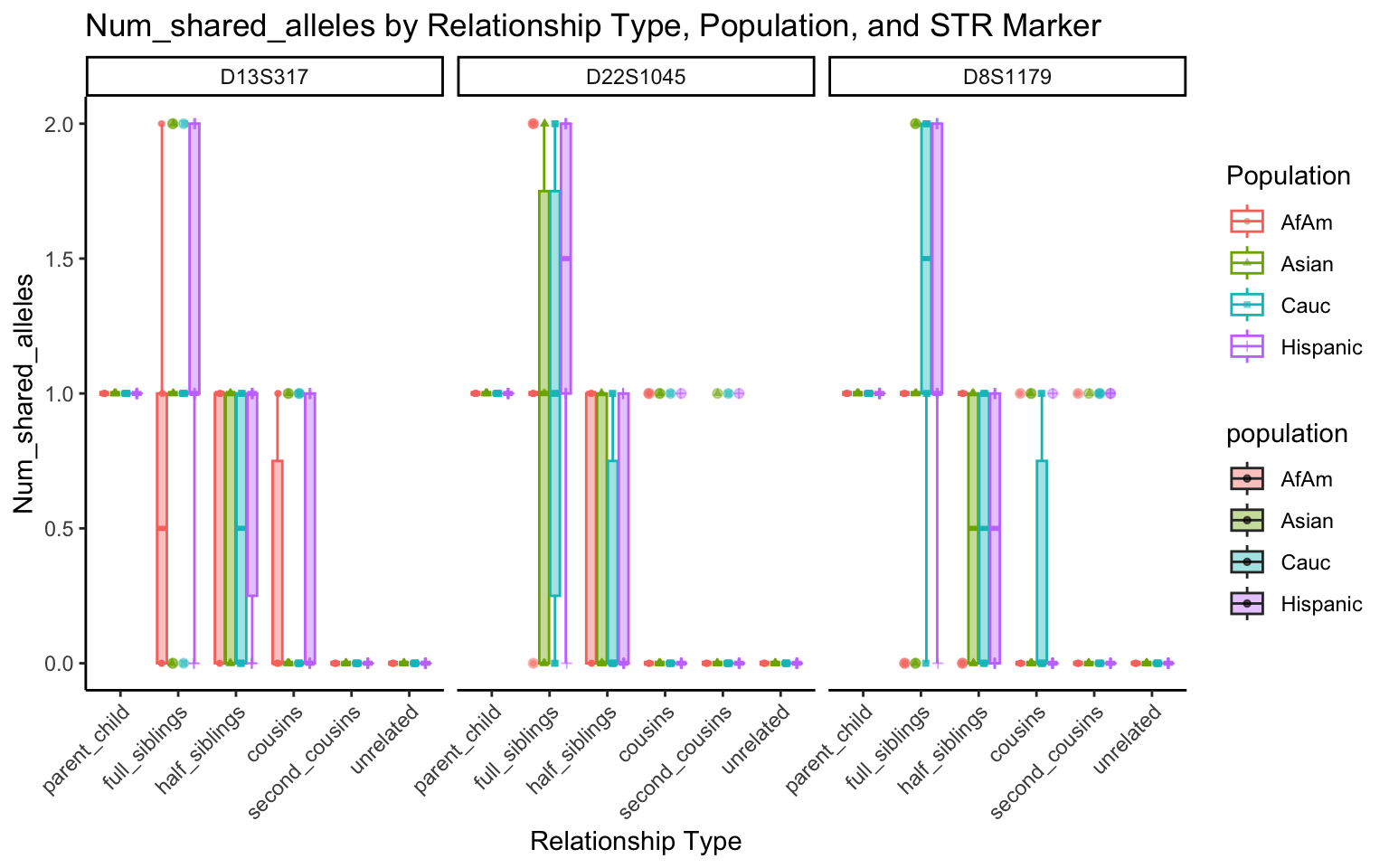
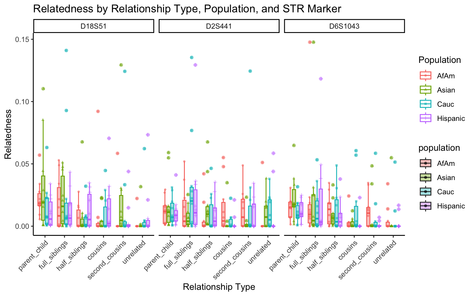
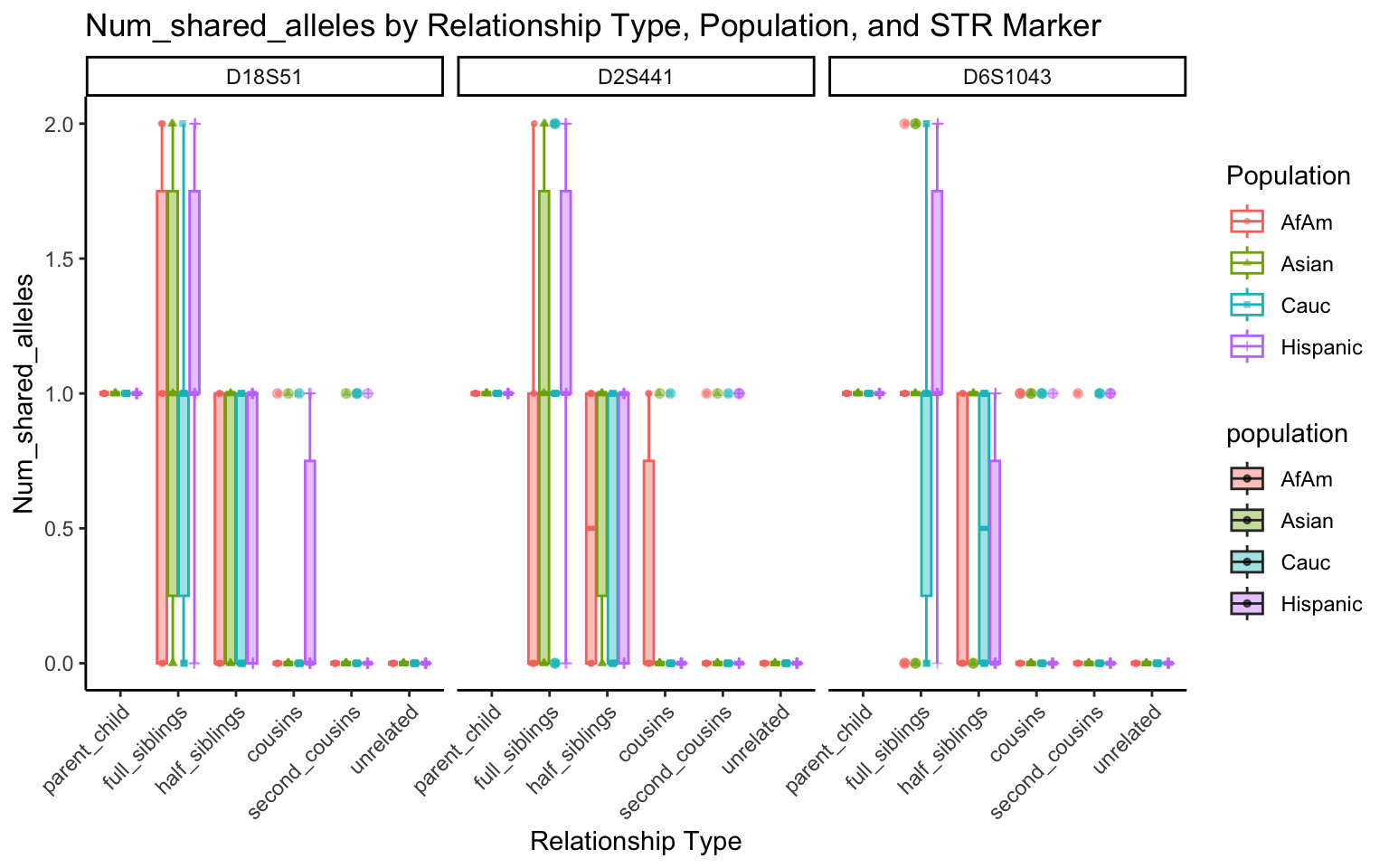
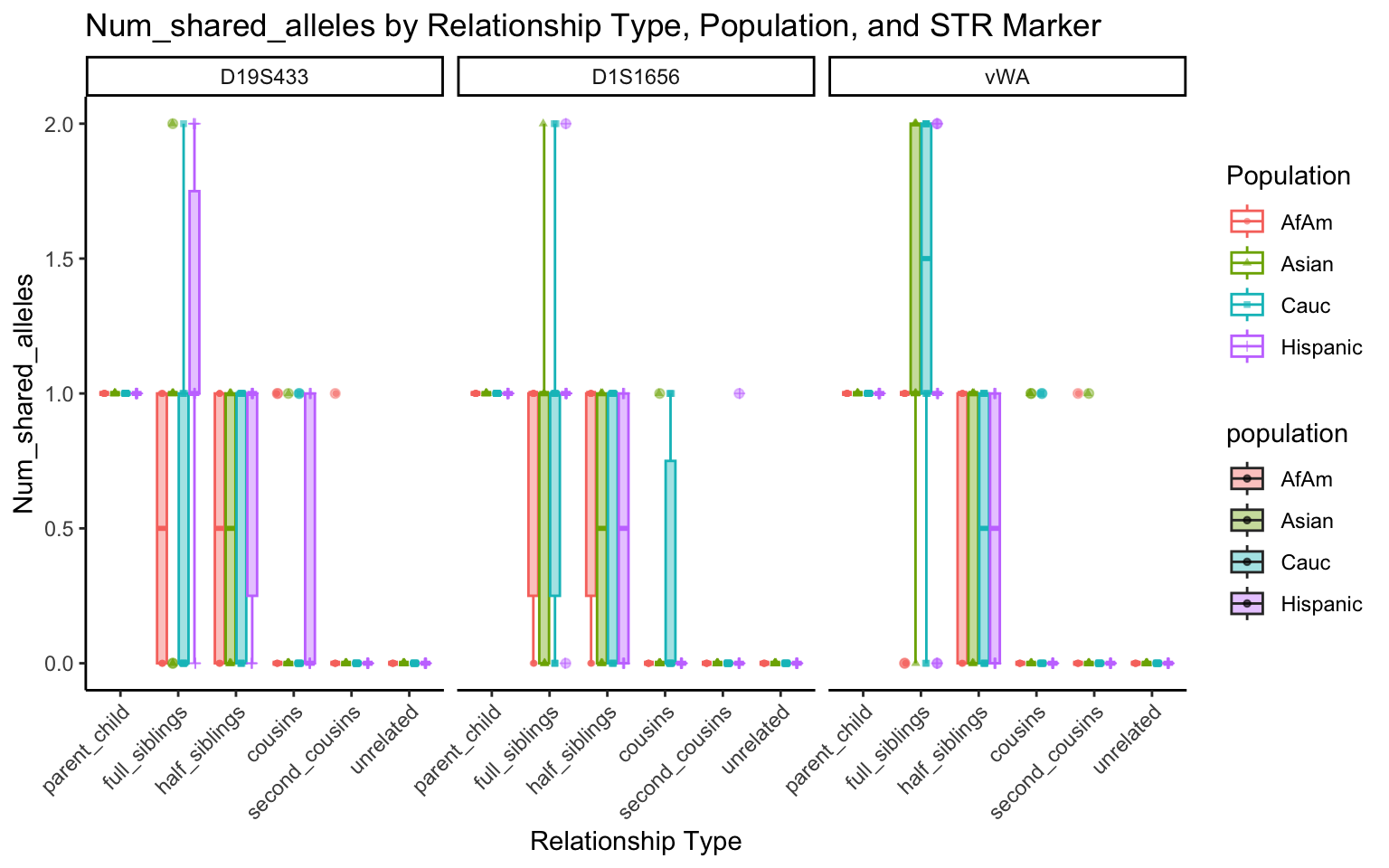
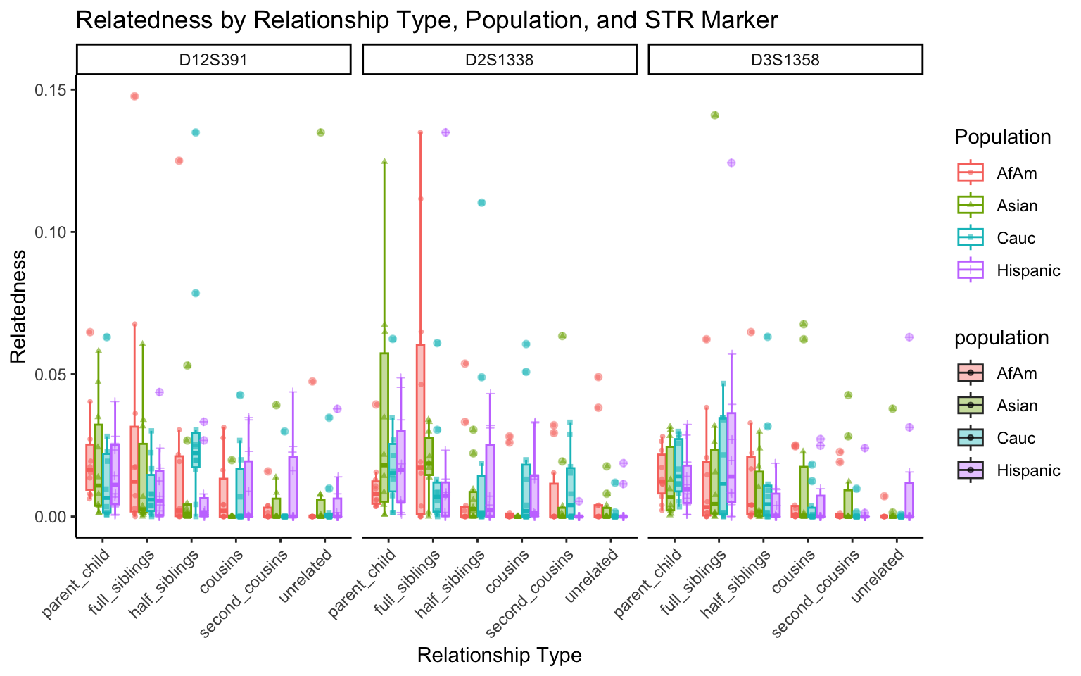
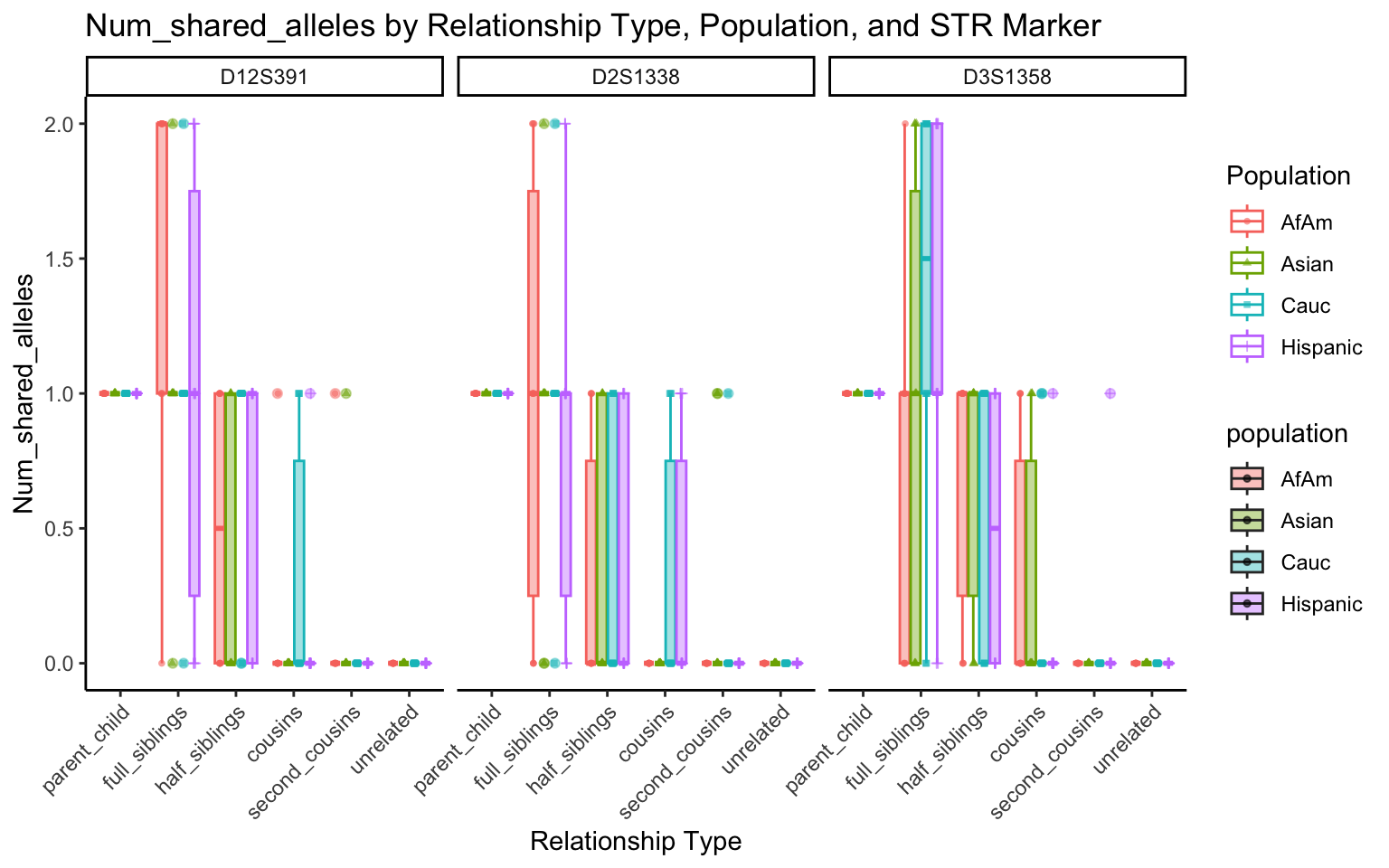
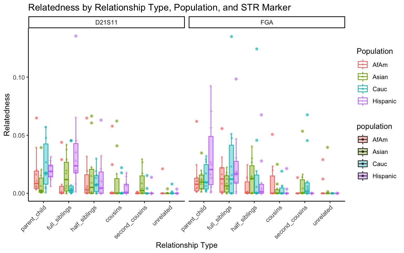
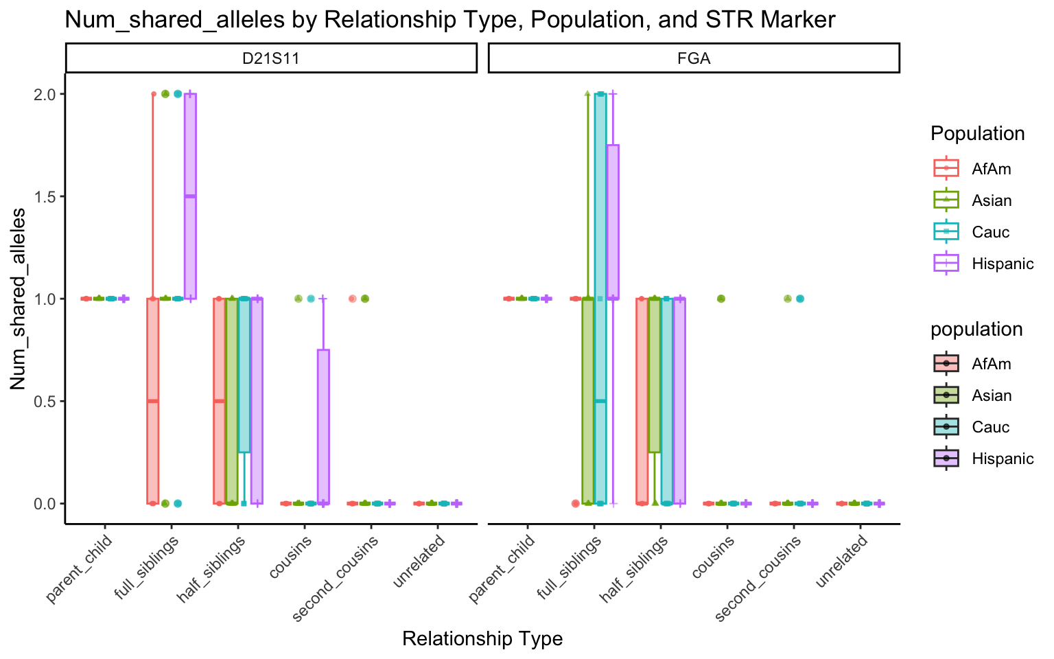
create_plot <- function(df, variable_to_plot) {
  # Create the plot
  p <- ggplot(df, aes(x = relationship_type, y = .data[[variable_to_plot]], color = population, shape = population, fill = population)) +
    geom_boxplot(alpha = 0.4) + # Change the order of geom_boxplot() and geom_point() and adjust alpha
    geom_point(position = position_jitterdodge(jitter.width = 0.1, dodge.width = 0.75), size = 1, alpha = 0.6) +
    facet_grid(. ~ marker) +
    theme_classic() +
    theme(axis.text.x = element_text(angle = 45, hjust = 1)) +
    scale_x_discrete(limits = c('parent_child', 'full_siblings', 'half_siblings', 'cousins', 'second_cousins', 'unrelated')) +
    labs(title = paste(ucfirst(variable_to_plot), "by Relationship Type, Population, and STR Marker"),
         x = "Relationship Type", 
         y = ucfirst(variable_to_plot), 
         color = "Population",
         shape = "Population")
  
  return(p)
}

# Filter your data for the first 3 unique STR markers
factor_vars <- c("marker", "population", "relationship_type")
numeric_vars <- c("relatedness", "num_shared_alleles")

# Filter your data for unique STR markers and remove the "all" population
results_df_filtered <- results_df %>%
  filter(population != "all") %>%
  mutate(
    across(all_of(factor_vars), as.factor),
    across(all_of(numeric_vars), as.numeric)
  )

# Find the total number of unique markers
total_markers <- length(unique(results_df_filtered$marker))

# Iterate through the unique markers in groups of 3
for (i in seq(1, total_markers, by = 3)) {
  # Filter the data for the current set of 3 or fewer markers
  filtered_results_df <- results_df_filtered %>%
    filter(marker %in% unique(marker)[i:min(i+2, total_markers)])
  
  # Create and display the plots for the current set of markers
  for (variable_to_plot in c("relatedness", "num_shared_alleles")) {
    plot <- create_plot(df = filtered_results_df, variable_to_plot = variable_to_plot)
    print(plot) # Print the plot to display it in the RMarkdown document
  }
}

Version	Author	Date
8a464dc	Tina Lasisi	2024-01-18

Version	Author	Date
8a464dc	Tina Lasisi	2024-01-18

Version	Author	Date
8a464dc	Tina Lasisi	2024-01-18

Version	Author	Date
8a464dc	Tina Lasisi	2024-01-18

Version	Author	Date
8a464dc	Tina Lasisi	2024-01-18

Version	Author	Date
8a464dc	Tina Lasisi	2024-01-18

Version	Author	Date
8a464dc	Tina Lasisi	2024-01-18

Version	Author	Date
8a464dc	Tina Lasisi	2024-01-18

Version	Author	Date
8a464dc	Tina Lasisi	2024-01-18

Version	Author	Date
8a464dc	Tina Lasisi	2024-01-18

Version	Author	Date
8a464dc	Tina Lasisi	2024-01-18

Version	Author	Date
8a464dc	Tina Lasisi	2024-01-18

Version	Author	Date
8a464dc	Tina Lasisi	2024-01-18

Version	Author	Date
8a464dc	Tina Lasisi	2024-01-18

Version	Author	Date
8a464dc	Tina Lasisi	2024-01-18

Version	Author	Date
8a464dc	Tina Lasisi	2024-01-18

Version	Author	Date
8a464dc	Tina Lasisi	2024-01-18

Version	Author	Date
8a464dc	Tina Lasisi	2024-01-18

Version	Author	Date
8a464dc	Tina Lasisi	2024-01-18

Version	Author	Date
8a464dc	Tina Lasisi	2024-01-18

All Markers together

# Function to simulate genotypes for a pair of individuals for all markers
simulate_genotypes_all_markers <- function(df, relationship_type, population) {
  markers <- unique(df$marker)
  
  # Simulate the first individual's alleles by drawing from the population frequency for each marker
  individual1 <- setNames(lapply(markers, function(marker) {
    allele_frequencies <- df %>%
      filter(marker == marker, population == population) %>%
      pull(frequency) %>%
      setNames(df$allele)
      
    sample(names(allele_frequencies), size = 2, replace = TRUE, prob = allele_frequencies)
  }), markers)
  
  # Relationship probabilities
  relationship_probs <- list(
    'parent_child' = c(0, 1, 0),
    'full_siblings' = c(1/4, 1/2, 1/4),
    'half_siblings' = c(1/2, 1/2, 0),
    'cousins' = c(7/8, 1/8, 0),
    'second_cousins' = c(15/16, 1/16, 0),
    'unrelated' = c(1, 0, 0)
  )
  
  prob_shared_alleles <- relationship_probs[[relationship_type]]
  num_shared_alleles <- sample(c(0, 1, 2), size = 1, prob = prob_shared_alleles)
  
  individual2 <- setNames(lapply(markers, function(marker) {
  allele_frequencies <- df %>%
    filter(marker == marker, population == population) %>%
    arrange(marker, allele) %>%
    pull(frequency) %>%
    setNames(df$allele)
  
  prob_shared_alleles <- relationship_probs[[relationship_type]]
  non_zero_indices <- which(prob_shared_alleles != 0)
  num_shared_alleles <- sample(non_zero_indices - 1, size = 1, prob = prob_shared_alleles[non_zero_indices])

  alleles_from_individual1 <- sample(individual1[[marker]], size = num_shared_alleles)
  alleles_from_population <- sample(names(allele_frequencies), size = 2 - num_shared_alleles, replace = TRUE, prob = allele_frequencies)
  
  return(c(alleles_from_individual1, alleles_from_population))
}), markers)

  # Return the simulated genotypes
  return(list(individual1 = individual1, individual2 = individual2))
}



# Function to calculate the index of relatedness for all markers
calculate_relatedness_all_markers <- function(simulated_genotypes, df, population) {
  markers <- names(simulated_genotypes$individual1)
  
  # Calculate the number of shared alleles for each marker
  num_shared_alleles <- sapply(markers, function(marker) {
    sum(simulated_genotypes$individual1[[marker]] %in% simulated_genotypes$individual2[[marker]])
  })
  
  # Calculate the index of relatedness as the number of shared alleles weighted inversely to their frequencies
  # Now considering both individuals' alleles for the inverse frequency weighting
  relatedness <- sapply(markers, function(marker) {
    allele_frequencies <- df %>%
      filter(marker == marker, population == population) %>%
      pull(frequency) %>%
      setNames(df$allele)
      
    num_shared_alleles[marker] / (sum(1 / allele_frequencies[simulated_genotypes$individual1[[marker]]]) + sum(1 / allele_frequencies[simulated_genotypes$individual2[[marker]]]))
  })
  
  # Return the index of relatedness
  return(list(relatedness = relatedness, num_shared_alleles = num_shared_alleles))
  }

# Function to simulate genotypes and calculate relatedness for different relationships for all markers
simulate_relatedness_all_markers <- function(df, relationship_type, population) {
  # Simulate genotypes for all markers
  simulated_genotypes <- simulate_genotypes_all_markers(df, relationship_type, population)
  
  # Calculate and return the relatedness for all markers
  relatedness_data <- calculate_relatedness_all_markers(simulated_genotypes, df, population)
  
   # Before returning the results_df, add marker and population information
  results_df$marker <- rownames(results_df)
  results_df$population <- population
  
  return(relatedness_data)
}

Visualizations

# Define the list of relationship types
relationship_types <- c('parent_child', 'full_siblings', 'half_siblings', 'cousins', 'second_cousins', 'unrelated')

# Create a dataframe of all combinations of populations and relationship types
combinations <- expand.grid(population = unique(df$population), relationship_type = relationship_types)

# Apply the function to each combination
results <- combinations %>%
  split(seq(nrow(.))) %>%
  map_dfr(function(combination) {
    population <- combination$population
    relationship_type <- combination$relationship_type
    # cat("Processing:", "population =", population, "; relationship_type =", relationship_type, "\n")
    sim_results <- simulate_relatedness_all_markers(df, relationship_type[[1]], population[[1]])
    
    # Bind resulting data frames
    tibble(
      population = population,
      relationship_type = relationship_type,
      sim_results = list(sim_results)
    )
  })

multi_results <- results %>% 
  mutate(
    sum_relatedness = map_dbl(sim_results, function(x) {
      sum(x[["relatedness"]], na.rm = TRUE)
    }),
    sum_alleles = map_dbl(sim_results, function(x) {
      sum(x[["num_shared_alleles"]], na.rm = TRUE)
    })
  ) %>% 
  select(-sim_results)

multi_results

# A tibble: 30 × 4
   population relationship_type sum_relatedness sum_alleles
   <fct>      <fct>                       <dbl>       <dbl>
 1 AfAm       parent_child                0.589          31
 2 all        parent_child                0.843          32
 3 Asian      parent_child                0.501          35
 4 Cauc       parent_child                0.442          33
 5 Hispanic   parent_child                0.489          31
 6 AfAm       full_siblings               0.380          29
 7 all        full_siblings               0.704          40
 8 Asian      full_siblings               0.556          36
 9 Cauc       full_siblings               0.237          26
10 Hispanic   full_siblings               0.375          28
# ℹ 20 more rows

# Define the number of simulations
n_sims <- 10

# Define the list of relationship types
relationship_types <- c('parent_child', 'full_siblings', 'half_siblings', 'cousins', 'second_cousins', 'unrelated')

# Create a dataframe of all combinations of populations, relationship types, and simulations
combinations <- expand.grid(population = unique(df$population), relationship_type = relationship_types, simulation = 1:n_sims)

# Apply the function to each combination
results <- combinations %>%
  split(seq(nrow(.))) %>%
  map_dfr(function(combination) {
    population <- combination$population
    relationship_type <- combination$relationship_type
    sim <- combination$simulation
    # cat("Processing:", "population =", population, "; relationship_type =", relationship_type, "; simulation =", sim, "\n")
    sim_results <- simulate_relatedness_all_markers(df, relationship_type[[1]], population[[1]])
    
    # Bind resulting data frames
    tibble(
      population = population,
      relationship_type = relationship_type,
      simulation = sim,
      sim_results = list(sim_results)
    )
  })

multi_results <- results %>% 
  mutate(
    sum_relatedness = map_dbl(sim_results, function(x) {
      sum(x[["relatedness"]], na.rm = TRUE)
    }),
    sum_alleles = map_dbl(sim_results, function(x) {
      sum(x[["num_shared_alleles"]], na.rm = TRUE)
    })
  ) %>% 
  select(-sim_results)

multi_results

# A tibble: 300 × 5
   population relationship_type simulation sum_relatedness sum_alleles
   <fct>      <fct>                  <int>           <dbl>       <dbl>
 1 AfAm       parent_child               1           0.532          31
 2 all        parent_child               1           0.438          31
 3 Asian      parent_child               1           0.388          32
 4 Cauc       parent_child               1           0.368          30
 5 Hispanic   parent_child               1           0.411          33
 6 AfAm       full_siblings              1           0.373          25
 7 all        full_siblings              1           0.717          35
 8 Asian      full_siblings              1           0.681          29
 9 Cauc       full_siblings              1           0.426          24
10 Hispanic   full_siblings              1           0.516          32
# ℹ 290 more rows

create_plot <- function(df, variable_to_plot) {
  # Create the plot
  p <- ggplot(df, aes(x = relationship_type, y = .data[[variable_to_plot]], color = population, shape = population, fill = population)) +
    geom_boxplot(alpha = 0.4, position = position_dodge(width = 0.75)) +
    geom_point(position = position_jitterdodge(jitter.width = 0.1, dodge.width = 0.75), size = 1, alpha = 0.6) +
    theme_classic() +
    theme(axis.text.x = element_text(angle = 45, hjust = 1)) +
    scale_x_discrete(limits = c('parent_child', 'full_siblings', 'half_siblings', 'cousins', 'second_cousins', 'unrelated')) +
    labs(title = paste(ucfirst(variable_to_plot), "by Relationship Type and Population"),
         x = "Relationship Type", 
         y = ucfirst(variable_to_plot), 
         color = "Population",
         shape = "Population")
  
  return(p)
}

# Filter your data for unique STR markers and remove the "all" population
df_plt_multi_results <- multi_results %>%
  filter(population != "all") %>%
  select(-simulation)

p <- create_plot(df_plt_multi_results, "sum_relatedness")
p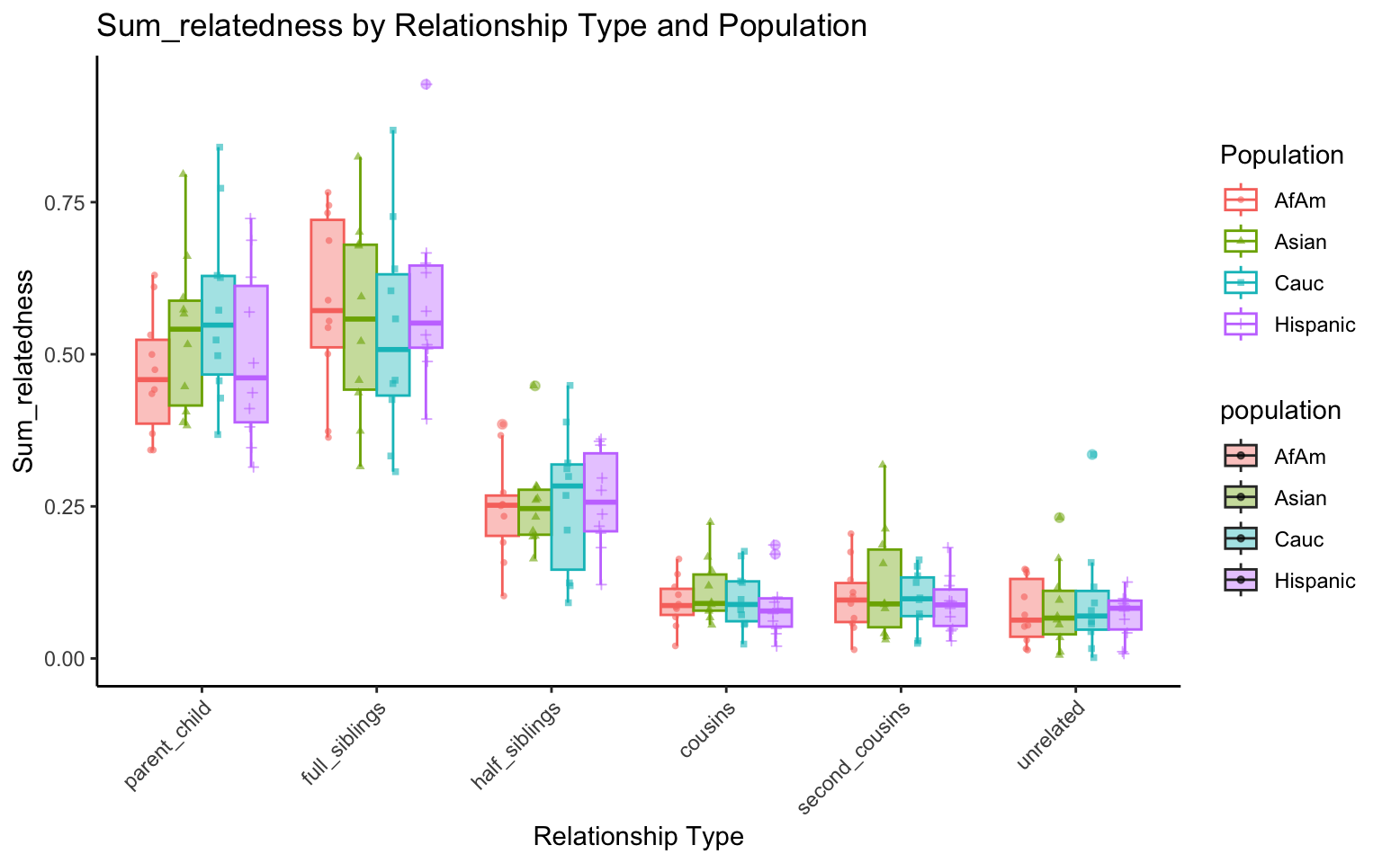

Version	Author	Date
8a464dc	Tina Lasisi	2024-01-18

plt_allele <- create_plot(df_plt_multi_results, "sum_alleles")

plt_allele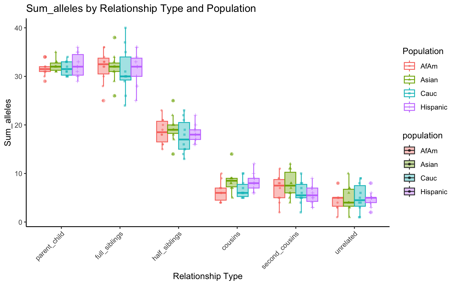

Version	Author	Date
8a464dc	Tina Lasisi	2024-01-18

Updated LR

From Weight-of-evidence for forensic DNA profiles book

Likelihood ratio for a single locus is:

\[ R=\kappa_0+\kappa_1 / R_X^p+\kappa_2 / R_X^u \] Where \(\kappa\) is the probability of having 0, 1 or 2 alleles IBD for a given relationship.

The \(R_X\) terms are quantifying the “surprisingness” of a particular pattern of allele sharing.

The \(R_X^p\) terms attached to the \(kappa_1\) are defined in the following table:

\[ \begin{aligned} &\text { Table 7.2 Single-locus LRs for paternity when } \mathcal{C}_M \text { is unavailable. }\\ &\begin{array}{llc} \hline c & Q & R_X \times\left(1+2 F_{S T}\right) \\ \hline \mathrm{AA} & \mathrm{AA} & 3 F_{S T}+\left(1-F_{S T}\right) p_A \\ \mathrm{AA} & \mathrm{AB} & 2\left(2 F_{S T}+\left(1-F_{S T}\right) p_A\right) \\ \mathrm{AB} & \mathrm{AA} & 2\left(2 F_{S T}+\left(1-F_{S T}\right) p_A\right) \\ \mathrm{AB} & \mathrm{AC} & 4\left(F_{S T}+\left(1-F_{S T}\right) p_A\right) \\ \mathrm{AB} & \mathrm{AB} & 4\left(F_{S T}+\left(1-F_{S T}\right) p_A\right)\left(F_{S T}+\left(1-F_{S T}\right) p_B\right) /\left(2 F_{S T}+\left(1-F_{S T}\right)\left(p_A+p_B\right)\right) \\ \hline \end{array} \end{aligned} \]

For our purposes we will take out the \(F_{S T}\) values. So the table will be as follows:

\[ \begin{aligned} &\begin{array}{llc} \hline c & Q & R_X \\ \hline \mathrm{AA} & \mathrm{AA} & p_A \\ \mathrm{AA} & \mathrm{AB} & 2 p_A \\ \mathrm{AB} & \mathrm{AA} & 2p_A \\ \mathrm{AB} & \mathrm{AC} & 4p_A \\ \mathrm{AB} & \mathrm{AB} & 4 p_A p_B/(p_A+p_B) \\ \hline \end{array} \end{aligned} \]

If none of the alleles match, then the \(\kappa_1 / R_X^p = 0\).

The \(R_X^u\) terms attached to the \(kappa_2\) are defined as:

If both alleles match and are homozygous the equation is 6.4 (pg 85). Single locus match probability: \(\mathrm{CSP}=\mathcal{G}_Q=\mathrm{AA}\) \[ \frac{\left(2 F_{S T}+\left(1-F_{S T}\right) p_A\right)\left(3 F_{S T}+\left(1-F_{S T}\right) p_A\right)}{\left(1+F_{S T}\right)\left(1+2 F_{S T}\right)} \] Simplified to: \[ p_A{ }^2 \]

If both alleles match and are heterozygous, the equation is 6.5 (pg 85) Single locus match probability: \(\mathrm{CSP}=\mathcal{G}_Q=\mathrm{AB}\) \[ 2 \frac{\left(F_{S T}+\left(1-F_{S T}\right) p_A\right)\left(F_{S T}+\left(1-F_{S T}\right) p_B\right)}{\left(1+F_{S T}\right)\left(1+2 F_{S T}\right)} \] Simplified to:

\[ 2 p_A p_B \] If both alleles do not match then \(\kappa_2 / R_X^u = 0\).

Calculating LR

We need 100,000 unrelated pairs.

sessionInfo()

R version 4.3.2 (2023-10-31)
Platform: aarch64-apple-darwin20 (64-bit)
Running under: macOS Sonoma 14.2.1

Matrix products: default
BLAS:   /Library/Frameworks/R.framework/Versions/4.3-arm64/Resources/lib/libRblas.0.dylib 
LAPACK: /Library/Frameworks/R.framework/Versions/4.3-arm64/Resources/lib/libRlapack.dylib;  LAPACK version 3.11.0

locale:
[1] en_US.UTF-8/en_US.UTF-8/en_US.UTF-8/C/en_US.UTF-8/en_US.UTF-8

time zone: America/Detroit
tzcode source: internal

attached base packages:
[1] stats     graphics  grDevices utils     datasets  methods   base     

other attached packages:
 [1] lubridate_1.9.3 forcats_1.0.0   stringr_1.5.1   dplyr_1.1.4    
 [5] purrr_1.0.2     readr_2.1.5     tidyr_1.3.0     tibble_3.2.1   
 [9] ggplot2_3.4.4   tidyverse_2.0.0 readxl_1.4.3    workflowr_1.7.1

loaded via a namespace (and not attached):
 [1] gtable_0.3.4      xfun_0.41         bslib_0.6.1       processx_3.8.3   
 [5] callr_3.7.3       tzdb_0.4.0        vctrs_0.6.5       tools_4.3.2      
 [9] ps_1.7.5          generics_0.1.3    parallel_4.3.2    fansi_1.0.6      
[13] highr_0.10        pkgconfig_2.0.3   lifecycle_1.0.4   compiler_4.3.2   
[17] farver_2.1.1      git2r_0.33.0      munsell_0.5.0     getPass_0.2-4    
[21] httpuv_1.6.13     htmltools_0.5.7   sass_0.4.8        yaml_2.3.8       
[25] later_1.3.2       pillar_1.9.0      crayon_1.5.2      jquerylib_0.1.4  
[29] whisker_0.4.1     cachem_1.0.8      tidyselect_1.2.0  digest_0.6.34    
[33] stringi_1.8.3     labeling_0.4.3    rprojroot_2.0.4   fastmap_1.1.1    
[37] grid_4.3.2        colorspace_2.1-0  cli_3.6.2         magrittr_2.0.3   
[41] utf8_1.2.4        withr_2.5.2       scales_1.3.0      promises_1.2.1   
[45] bit64_4.0.5       timechange_0.2.0  rmarkdown_2.25    httr_1.4.7       
[49] bit_4.0.5         cellranger_1.1.0  hms_1.1.3         evaluate_0.23    
[53] knitr_1.45        rlang_1.1.3       Rcpp_1.0.12       glue_1.7.0       
[57] rstudioapi_0.15.0 vroom_1.6.5       jsonlite_1.8.8    R6_2.5.1         
[61] fs_1.6.3