Main simulation study
Scenario 1
The simulated data in this example are generated to demonstrate how to use the KODAMA and UMAP techniques for cluster and spatial domain analysis. We create two distinct regions representing areas rich in T cells and B cells within the lymph node. We generate x and y coordinates for the two regions, assigning labels to simulate different cell types (T cells and B cells).
library("KODAMA")
library("KODAMAextra")
x1=runif(100,min=-1,max=0)
x2=runif(100,min=0,max=1)
y1=runif(100)
y2=runif(100)
x=c(x1,x2)
y=c(y1,y2)
xy=cbind(x,y)

labels=rep(c(TRUE,FALSE),each=100)
ss=sample(100,5)
labels[ss]=!labels[ss]
labels=labels
region=rep(1:0,each=100)

data=cbind(rnorm(200,mean=labels,sd=0.1),
           rnorm(200,mean=labels,sd=0.1))

color.code=c("#1d79d0aa","#53ca3eaa")
Visualization with KODAMA and UMAP
We use KODAMA and UMAP methods to analyze and visualize the data, applying dimensionality reduction and identifying clusters and spatial domains.
kk <- KODAMA.matrix.parallel(data,spatial=xy,spatial.resolution=0.1,M=100,
                      FUN="PLS",
                      landmarks = 100000,
                      splitting = 100,
                      f.par.pls =  2,
                      n.cores=4)
socket cluster with 4 nodes on host 'localhost'
================================================================================[1] "Finished parallel computation"
[1] "Calculation of dissimilarity matrix..."
================================================================================vis=RunKODAMAvisualization(kk,method="UMAP")
u=umap(data)$layout
par(mfrow=c(1,3))
plot(x,y,bg=color.code[region+1],pch=21+2*!labels,cex=1+1.5*region,axes=FALSE,main="Position")
axis(1)
axis(2,las=2)
box()
plot(vis,type="n",axes=FALSE,main="KODAMA")
axis(1)
axis(2,las=2)
box()
points(vis[!labels,],bg=color.code[region+1][!labels],pch=21+2,cex=1+1.5*region[!labels])
points(vis[labels,],bg=color.code[region+1][labels],pch=21+2*0,cex=1+1.5*region[labels])
plot(u,type="n",axes=FALSE,xlab="Dimension 1",ylab="Dimension 2",main="UMAP")
axis(1)
axis(2,las=2)
box()
points(u[!labels,],bg=color.code[region+1][!labels],pch=21+2,cex=1+1.5*region[!labels])
points(u[labels,],bg=color.code[region+1][labels],pch=21+2*0,cex=1+1.5*region[labels])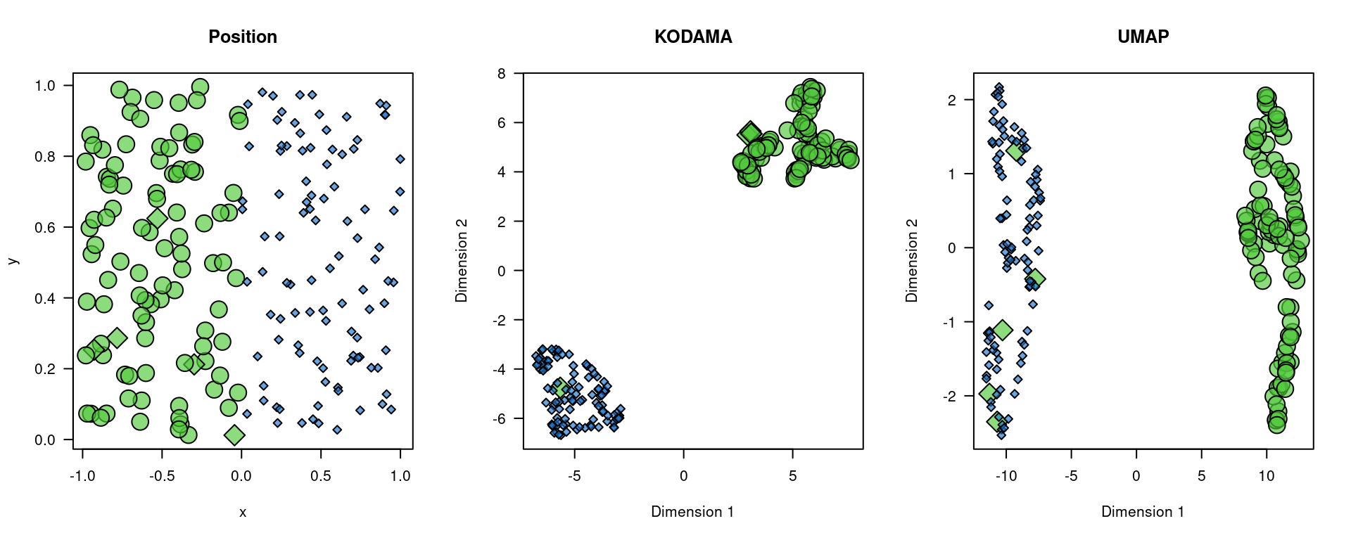
| Version | Author | Date |
|---|---|---|
| 6f7daac | Stefano Cacciatore | 2024-07-19 |
The generated visualizations show the position of the points, as well as the results of the KODAMA and UMAP analyses. The visualizations indicate the molecular positions and identified clusters, providing a better understanding of the spatial structure of the immune cells within the lymph node. This can help identify regions of interest for further analysis, with significant implications for research in immunology and the development of targeted therapies.
Scenario 2
In this section, we build upon the previous data generation and visualization methods to demonstrate advanced manipulations and visualizations using KODAMA and UMAP techniques.
Data Generation and Setting the Random Seed
Continuing from the previous section, we set the random seed and generate data for two distinct regions, assigning labels and specific regions to each data point.
x1=runif(100,min=-1,max=0)
x2=runif(100,min=0,max=1)
y1=runif(100)
y2=runif(100)
x=c(x1,x2)
y=c(y1,y2)
xy=cbind(x,y)


labels=rep(c(TRUE,FALSE),each=100)

region=rep(1:0,each=100)

data=cbind(rnorm(200,mean=1+labels,sd=0.1),
           rnorm(200,mean=1+labels,sd=0.1),
           rnorm(200,mean=1+labels,sd=0.1),
           rnorm(200,mean=1+labels,sd=0.1))

ll=length(data)
ss=sample(ll,ll*0.5)
data[ss]=0
color.code=c("#1d79d0aa","#53ca3eaa")

sel=apply(data,1,function(x) sum(x>0))>2
data=data[sel,]
region=region[sel]
labels=labels[sel]
xy=xy[sel,]


labels=data>0
labels=labels[,1]+
  labels[,2]*2+
  labels[,3]*4+
  labels[,4]*8
labels=as.numeric(as.factor(labels))+1
Visualization with KODAMA and UMAP
We apply Principal Component Analysis (PCA) on the filtered data and use KODAMA and UMAP methods to analyze and visualize the data, applying dimensionality reduction and identifying clusters and spatial domains
pca=prcomp(scale(data))$x

kk <- KODAMA.matrix.parallel(pca,spatial=xy,spatial.resolution=0.1,M=100,
                             FUN="PLS",
                             landmarks = 100000,
                             splitting = 100,
                             f.par.pls =  10,
                             n.cores=4)
The number of components selected for PLS-DA is too high and it will be automatically reduced to 4socket cluster with 4 nodes on host 'localhost'
================================================================================[1] "Finished parallel computation"
[1] "Calculation of dissimilarity matrix..."
================================================================================config=umap.defaults
config$n_neighbors=15
vis=RunKODAMAvisualization(kk,method="UMAP",config=config)
u=umap(pca)$layout
old.par = par(mfrow=c(1,3))
plot(xy,bg=labels,pch=21+2*(region),cex=2+1*region,axes=FALSE,main="Position")
axis(1)
axis(2,las=2)
box()
plot(vis,bg=labels,pch=21+2*(region),cex=1+1.5*region,axes=FALSE,main="KODAMA")
axis(1)
axis(2,las=2)
box()
plot(u,bg=labels,pch=21+2*(region),cex=1+1.5*region,axes=FALSE,main="UMAP")
axis(1)
axis(2,las=2)
box()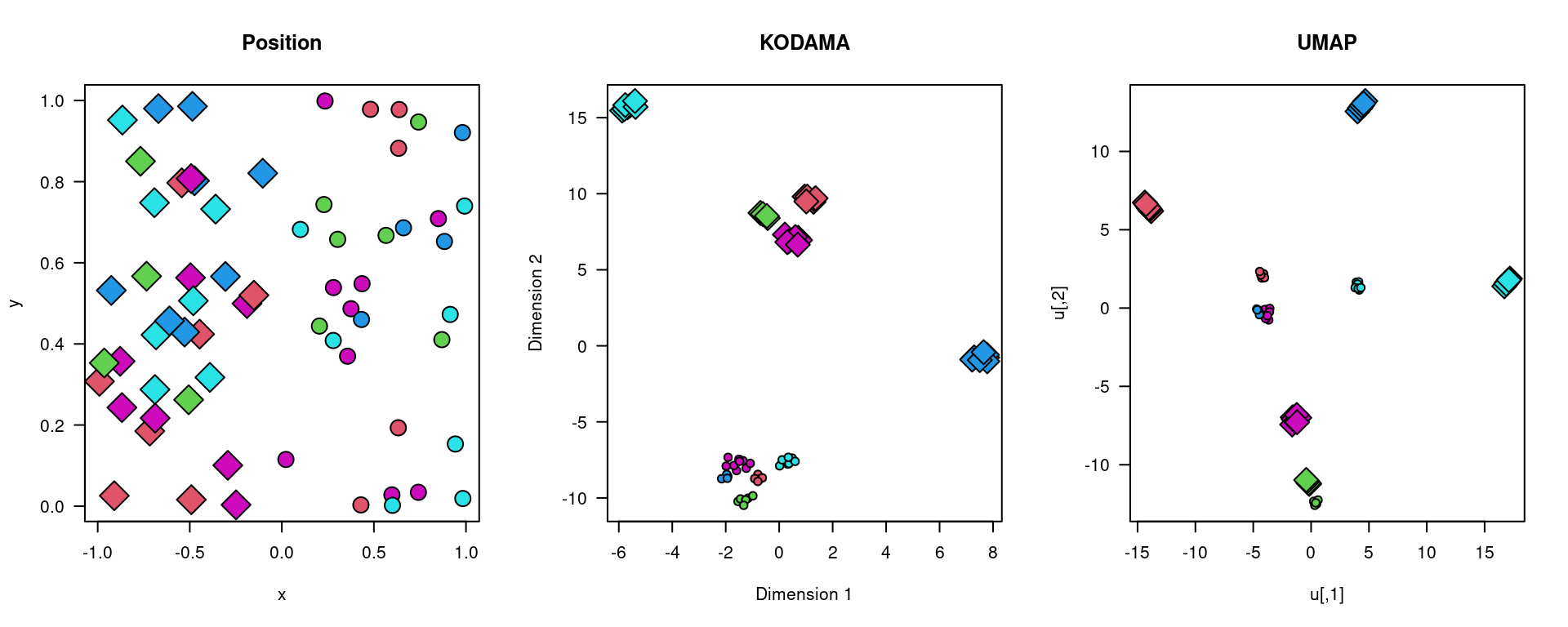
| Version | Author | Date |
|---|---|---|
| 6f7daac | Stefano Cacciatore | 2024-07-19 |
par(old.par)By integrating advanced manipulations and visualizations, we gain deeper insights into spatial data analysis, providing a foundation for further exploration and research in complex biological systems.
sessionInfo()R version 4.4.1 (2024-06-14)
Platform: x86_64-pc-linux-gnu
Running under: Ubuntu 20.04.6 LTS
Matrix products: default
BLAS: /usr/lib/x86_64-linux-gnu/blas/libblas.so.3.9.0
LAPACK: /usr/lib/x86_64-linux-gnu/lapack/liblapack.so.3.9.0
locale:
[1] LC_CTYPE=en_US.UTF-8 LC_NUMERIC=C
[3] LC_TIME=en_US.UTF-8 LC_COLLATE=en_US.UTF-8
[5] LC_MONETARY=en_US.UTF-8 LC_MESSAGES=en_US.UTF-8
[7] LC_PAPER=en_US.UTF-8 LC_NAME=C
[9] LC_ADDRESS=C LC_TELEPHONE=C
[11] LC_MEASUREMENT=en_US.UTF-8 LC_IDENTIFICATION=C
time zone: Etc/UTC
tzcode source: system (glibc)
attached base packages:
[1] parallel stats graphics grDevices utils datasets methods
[8] base
other attached packages:
[1] KODAMAextra_1.0 e1071_1.7-14 doParallel_1.0.17 iterators_1.0.14
[5] foreach_1.5.2 KODAMA_3.1 umap_0.2.10.0 Rtsne_0.17
[9] minerva_1.5.10 workflowr_1.7.1
loaded via a namespace (and not attached):
[1] sass_0.4.9 utf8_1.2.4 class_7.3-22 stringi_1.8.4
[5] lattice_0.22-6 digest_0.6.36 magrittr_2.0.3 evaluate_0.24.0
[9] grid_4.4.1 fastmap_1.2.0 rprojroot_2.0.4 jsonlite_1.8.8
[13] Matrix_1.7-0 processx_3.8.4 whisker_0.4.1 RSpectra_0.16-1
[17] doSNOW_1.0.20 ps_1.7.7 promises_1.3.0 httr_1.4.7
[21] fansi_1.0.6 codetools_0.2-20 jquerylib_0.1.4 cli_3.6.3
[25] rlang_1.1.4 cachem_1.1.0 yaml_2.3.9 tools_4.4.1
[29] httpuv_1.6.15 reticulate_1.38.0 vctrs_0.6.5 R6_2.5.1
[33] png_0.1-8 proxy_0.4-27 lifecycle_1.0.4 git2r_0.33.0
[37] stringr_1.5.1 fs_1.6.4 pkgconfig_2.0.3 callr_3.7.6
[41] pillar_1.9.0 bslib_0.7.0 later_1.3.2 glue_1.7.0
[45] Rcpp_1.0.12 highr_0.11 xfun_0.45 tibble_3.2.1
[49] rstudioapi_0.16.0 knitr_1.48 snow_0.4-4 htmltools_0.5.8.1
[53] rmarkdown_2.27 compiler_4.4.1 getPass_0.2-4 askpass_1.2.0
[57] openssl_2.2.0