About
Last updated: 2025-01-10
Checks: 7 0
Knit directory: KODAMA-Analysis/
This reproducible R Markdown analysis was created with workflowr (version 1.7.1). The Checks tab describes the reproducibility checks that were applied when the results were created. The Past versions tab lists the development history.
Great! Since the R Markdown file has been committed to the Git repository, you know the exact version of the code that produced these results.
Great job! The global environment was empty. Objects defined in the global environment can affect the analysis in your R Markdown file in unknown ways. For reproduciblity it’s best to always run the code in an empty environment.
The command set.seed(20240618) was run prior to running
the code in the R Markdown file. Setting a seed ensures that any results
that rely on randomness, e.g. subsampling or permutations, are
reproducible.
Great job! Recording the operating system, R version, and package versions is critical for reproducibility.
Nice! There were no cached chunks for this analysis, so you can be confident that you successfully produced the results during this run.
Great job! Using relative paths to the files within your workflowr project makes it easier to run your code on other machines.
Great! You are using Git for version control. Tracking code development and connecting the code version to the results is critical for reproducibility.
The results in this page were generated with repository version 86be707. See the Past versions tab to see a history of the changes made to the R Markdown and HTML files.
Note that you need to be careful to ensure that all relevant files for
the analysis have been committed to Git prior to generating the results
(you can use wflow_publish or
wflow_git_commit). workflowr only checks the R Markdown
file, but you know if there are other scripts or data files that it
depends on. Below is the status of the Git repository when the results
were generated:
Ignored files:
    Ignored:    .RData
    Ignored:    .Rhistory
    Ignored:    .Rproj.user/
    Ignored:    analysis/figure/

Untracked files:
    Untracked:  Elemina.RData
    Untracked:  KODAMA.svg
    Untracked:  Rplots.pdf
    Untracked:  code/Acinar_Cell_Carcinoma.ipynb
    Untracked:  code/Adenocarcinoma.ipynb
    Untracked:  code/Adjacent_normal_section.ipynb
    Untracked:  code/DLFPC_preprocessing.R
    Untracked:  code/DLPFC - BANKSY.R
    Untracked:  code/DLPFC - BASS.R
    Untracked:  code/DLPFC - BAYESPACE.R
    Untracked:  code/DLPFC - Nonspatial.R
    Untracked:  code/DLPFC - PRECAST.R
    Untracked:  code/DLPFC_comparison.R
    Untracked:  code/DLPFC_results_analysis.R
    Untracked:  code/VisiumHD-CRC.ipynb
    Untracked:  code/deep learning code DLPFC.R
    Untracked:  code/save tiles.py
    Untracked:  data/Adenocarcinoma.csv
    Untracked:  data/Annotations/
    Untracked:  data/DLFPC-Br5292-input.RData
    Untracked:  data/DLFPC-Br5595-input.RData
    Untracked:  data/DLFPC-Br8100-input.RData
    Untracked:  data/DLPFC-general.RData
    Untracked:  data/spots_classification_ALL.csv
    Untracked:  data/spots_classification_Acinar_Cell_Carcinoma.csv
    Untracked:  data/spots_classification_IF.csv
    Untracked:  data/spots_classification_Normal_prostate.csv
    Untracked:  data/trajectories.RData
    Untracked:  data/trajectories_VISIUMHD.RData
    Untracked:  output/BANSKY-results.RData
    Untracked:  output/BASS-results.RData
    Untracked:  output/BayesSpace-results.RData
    Untracked:  output/CRC-image.RData
    Untracked:  output/CRC-image2.RData
    Untracked:  output/CRC.png
    Untracked:  output/CRC2.png
    Untracked:  output/DL.RData
    Untracked:  output/DLFPC-All-2.RData
    Untracked:  output/DLFPC-All.RData
    Untracked:  output/DLFPC-Br5292.RData
    Untracked:  output/DLFPC-Br5595.RData
    Untracked:  output/DLFPC-Br8100.RData
    Untracked:  output/DLPFC1.svg
    Untracked:  output/DLPFC_all_cluster.svg
    Untracked:  output/Figure 1 - boxplot.pdf
    Untracked:  output/Figure 2 - DLPFC 10.pdf
    Untracked:  output/KODAMA-results.RData
    Untracked:  output/KODAMA_DLPFC_All_original.svg
    Untracked:  output/KODAMA_DLPFC_Br5595.svg
    Untracked:  output/KODAMA_DLPFC_Br5595_slide.svg
    Untracked:  output/MERFISH.RData
    Untracked:  output/Nonspatial-results.RData
    Untracked:  output/PRECAST-results.RData
    Untracked:  output/Prostate.RData
    Untracked:  output/VisiumHD3.RData
    Untracked:  output/a1.RData
    Untracked:  output/a2.RData
    Untracked:  output/a3.RData
    Untracked:  output/a4.RData
    Untracked:  output/a5.RData
    Untracked:  output/a6.RData
    Untracked:  output/a7.RData
    Untracked:  output/a8.RData
    Untracked:  output/image.RData
    Untracked:  output/pp.RData
    Untracked:  output/pp2.RData
    Untracked:  output/pp3.RData
    Untracked:  output/pp4.RData
    Untracked:  output/pp5.RData
    Untracked:  output/prostate1.svg
    Untracked:  output/prostate2.svg
    Untracked:  output/prostate3.svg
    Untracked:  output/prostate4.svg
    Untracked:  output/prostate5.svg
    Untracked:  output/prostate6.svg
    Untracked:  output/prostate7.svg
    Untracked:  output/tight_boundary.geojson
    Untracked:  remove.RData
    Untracked:  remove2.RData

Unstaged changes:
    Deleted:    analysis/D1.Rmd
    Deleted:    analysis/DLPFC-12.Rmd
    Deleted:    analysis/DLPFC-4.Rmd
    Deleted:    analysis/DLPFC1.Rmd
    Deleted:    analysis/DLPFC10.Rmd
    Deleted:    analysis/DLPFC2.Rmd
    Deleted:    analysis/DLPFC3.Rmd
    Deleted:    analysis/DLPFC4.Rmd
    Deleted:    analysis/DLPFC5.Rmd
    Deleted:    analysis/DLPFC6.Rmd
    Deleted:    analysis/DLPFC7.Rmd
    Deleted:    analysis/DLPFC8.Rmd
    Deleted:    analysis/DLPFC9.Rmd
    Deleted:    analysis/Du1.Rmd
    Deleted:    analysis/Du10.Rmd
    Deleted:    analysis/Du11.Rmd
    Deleted:    analysis/Du12.Rmd
    Deleted:    analysis/Du13.Rmd
    Deleted:    analysis/Du14.Rmd
    Deleted:    analysis/Du15.Rmd
    Deleted:    analysis/Du16.Rmd
    Deleted:    analysis/Du17.Rmd
    Deleted:    analysis/Du18.Rmd
    Deleted:    analysis/Du19.Rmd
    Deleted:    analysis/Du2.Rmd
    Deleted:    analysis/Du20.Rmd
    Deleted:    analysis/Du3.Rmd
    Deleted:    analysis/Du4.Rmd
    Deleted:    analysis/Du5.Rmd
    Deleted:    analysis/Du6.Rmd
    Deleted:    analysis/Du7.Rmd
    Deleted:    analysis/Du8.Rmd
    Deleted:    analysis/Du9.Rmd
    Modified:   analysis/Giotto.Rmd
    Modified:   analysis/Prostate.Rmd
    Deleted:    analysis/STARmap.Rmd
    Modified:   code/VisiumHD_CRC_download.sh
    Deleted:    data/Pathology.csv
Note that any generated files, e.g. HTML, png, CSS, etc., are not included in this status report because it is ok for generated content to have uncommitted changes.
These are the previous versions of the repository in which changes were
made to the R Markdown (analysis/VisiumHD.Rmd) and HTML
(docs/VisiumHD.html) files. If you’ve configured a remote
Git repository (see ?wflow_git_remote), click on the
hyperlinks in the table below to view the files as they were in that
past version.
| File | Version | Author | Date | Message |
|---|---|---|---|---|
| Rmd | 86be707 | Stefano Cacciatore | 2025-01-10 | Start my new project |
| Rmd | 7bba919 | Stefano Cacciatore | 2025-01-09 | Start my new project |
| html | a423e5f | Stefano Cacciatore | 2024-09-04 | Build site. |
| Rmd | b0a97fe | Stefano Cacciatore | 2024-09-04 | Start my new project |
| html | 9bdaa70 | Stefano Cacciatore | 2024-09-04 | Build site. |
| Rmd | ca72951 | Stefano Cacciatore | 2024-09-04 | Start my new project |
| html | 098b08e | Stefano Cacciatore | 2024-09-04 | Build site. |
| Rmd | eb8066e | Stefano Cacciatore | 2024-09-04 | Start my new project |
| html | 0010f3c | Stefano Cacciatore | 2024-09-04 | Build site. |
| Rmd | 3f515c0 | Stefano Cacciatore | 2024-09-04 | Start my new project |
| html | 51b0452 | Stefano Cacciatore | 2024-09-03 | Build site. |
| Rmd | c257b0e | Stefano Cacciatore | 2024-09-03 | Start my new project |
| Rmd | 22e2ac6 | Stefano Cacciatore | 2024-08-26 | Start my new project |
| html | d1192e9 | Stefano Cacciatore | 2024-08-12 | Build site. |
| Rmd | 5ef8148 | Stefano Cacciatore | 2024-08-12 | Start my new project |
| html | 3374e66 | Stefano Cacciatore | 2024-08-06 | Build site. |
| html | 35ce733 | Stefano Cacciatore | 2024-08-03 | Build site. |
| html | 82fe167 | Stefano Cacciatore | 2024-07-24 | Build site. |
| Rmd | b422e43 | Stefano Cacciatore | 2024-07-24 | Start my new project |
| html | 6f7daac | Stefano Cacciatore | 2024-07-19 | Build site. |
| Rmd | 5b97082 | tkcaccia | 2024-07-15 | updates |
| Rmd | 7be8f59 | tkcaccia | 2024-07-15 | updates |
| html | 7be8f59 | tkcaccia | 2024-07-15 | updates |
| Rmd | 79f73a2 | GitHub | 2024-07-14 | Update VisiumHD.Rmd |
| html | f8ca54a | tkcaccia | 2024-07-14 | update |
| html | d04c1e7 | GitHub | 2024-07-08 | Update VisiumHD.html |
| html | 754c8bf | GitHub | 2024-07-04 | Update VisiumHD.html |
| html | ee4ee17 | GitHub | 2024-06-19 | Add files via upload |
| Rmd | 615fc05 | GitHub | 2024-06-19 | Add files via upload |
Describe your project. The data can be downloaded using the following script: VisiumHD_CRC_download.sh. This script facilitates access to the raw data, which will then be preprocessed and analyzed in the subsequent steps of our pipeline.
The data can be downloaded using the following script: VisiumHD_CRC_download.sh. This script facilitates access to the raw data, which will then be preprocessed and analyzed in the subsequent steps of our pipeline.
library("ggplot2")
library("patchwork")
library("dplyr")
library("Seurat")
library("KODAMA")
library("KODAMAextra")
library("bigmemory")

localdir="../Colorectal/outs/"
object <- Load10X_Spatial(data.dir = localdir, bin.size = c(8))

image=as.raster(object@images$slice1.008um@image)
save(image,file="output/CRC-image.RData")
#object@images$slice1.008um@scale.factors$hires

# plot(image,xlim=c(320,530),ylim=c(200,410))
# points(xy[,2]*0.007973422,nrow(image)-xy[,1]*0.007973422,pch=20)

#xy=as.matrix(GetTissueCoordinates(sp_obj)[,1:2])

#image=as.raster(imgData(object)$data[[1]])

#xy_sel=spatialCoords(spe_sub)
#xy_sel=xy_sel*scaleFactors(spe_sub)
#xy_sel[,2]=nrow(image)-xy_sel[,2]


 vln.plot <- VlnPlot(object, features = "nCount_Spatial.008um", pt.size = 0) + NoLegend()
 count.plot <- SpatialFeaturePlot(object, features = "nCount_Spatial.008um", pt.size.factor = 1.2) +
   theme(legend.position = "right")

nCount_Spatial=colSums(object@assays$Spatial.008um$counts)
#w= which(nCount_Spatial >10)
#object@assays$Spatial.008um$counts= object@assays$Spatial.008um$counts[,w]
#object@meta.data=object@meta.data[w,]

sp_obj <- subset(
  object,
  subset = nCount_Spatial.008um > 100)


nCount_Spatial=colSums(sp_obj@assays$Spatial.008um$counts)


 counts=sp_obj@assays$Spatial.008um$counts
 is_mito <- grepl("(^MT-)|(^mt-)", rownames(counts))
 counts <- counts[!is_mito,]

 filter_genes_ncounts=1
 filter_genes_pcspots=0.5
 nspots <- ceiling(filter_genes_pcspots/100 *  ncol(counts))
 ix_remove <- rowSums(counts >= filter_genes_ncounts) <   nspots
 counts <- counts[!ix_remove,]

 QCgenes <- rownames(counts)

 VariableFeatures(sp_obj) = QCgenes

 rm(counts)


DefaultAssay(sp_obj) <- "Spatial.008um"
sp_obj <- NormalizeData(sp_obj)


sp_obj <- FindVariableFeatures(sp_obj)
sp_obj <- ScaleData(sp_obj)

xy=as.matrix(GetTissueCoordinates(sp_obj)[,1:2])

sp_obj <- RunPCA(sp_obj, reduction.name = "pca.008um")

dim(sp_obj)
[1] 18085 428381plot(Seurat::Embeddings(sp_obj, reduction = "pca.008um"))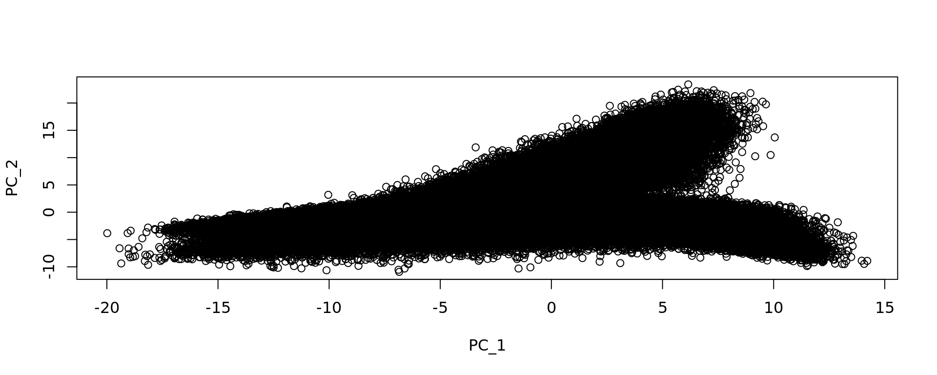
#sp_obj <- RunKODAMAmatrix(sp_obj, reduction = "pca.008um",
#                          FUN= "PLS" ,
#                          landmarks = 10000,
#                          splitting = 100,
#                          f.par.pls = 50,
#                          spatial.resolution = 0.4,
#                          n.cores=8)

#  print("KODAMA finished")

#     config=umap.defaults
#     config$n_threads = 8
#     config$n_sgd_threads = "auto"
#     sp_obj <- RunKODAMAvisualization(sp_obj, method = "UMAP",config=config)


# kk_UMAP=Seurat::Embeddings(sp_obj, reduction = "KODAMA")

# save(kk_UMAP,xy,file="output/VisiumHD.RData")

load("output/VisiumHD3.RData")

rr=read.csv("data/spots_classification_ALL.csv",sep=",")
ss=strsplit(rr[,2],":")
ss=unlist(lapply(ss, function(x) x[2]))
ss=strsplit(ss,",")
ss=unlist(lapply(ss, function(x) x[1]))
ss=gsub("\"","",ss)

rr[,2]=ss
n=ave(1:length(rr[,1]), rr[,1], FUN = seq_along)
rr=rr[n==1,]
rownames(rr)=rr[,1]
rr=rr[rownames(kk_UMAP),]

  rr[rr==" blood vessel"]="blood vessel"
  rr[rr==" blood vessels"]="blood vessel"
  rr[rr==" cabilari"]="lymphovascular channels"
  rr[rr==" desmoplastic mecuosa"]="desmoplastic submucosa"
  rr[rr==" desmoplastic submucosa"]="desmoplastic submucosa"
  rr[rr==" dysplasia"]="dysplasia"
  rr[rr==" dysplasia_to_verify"]="intermediate dysplasia"
  rr[rr==" dystrophic calcification"]="dystrophic calcification"
  rr[rr==" exocrine duct"]="exocrine duct"
  rr[rr==" external glands"]="external glands"
  rr[rr==" high-grade dysplasia"]="high-grade dysplasia"
  rr[rr==" Immune cells"]="immune cells"
  rr[rr==" Invasive_carcinoma"]="invasive carcinoma"
  rr[rr==" lamina propria dysplasia"]="lamina propria dysplasia"
  rr[rr==" lymphovascular channels"]="lymphovascular channels"
  rr[rr==" muscularis mucosa"]="muscularis mucosa"
  rr[rr==" muscularis propria"]="muscularis propria"
  rr[rr==" Nerve fibers"]="nerve fibers"
  rr[rr==" normal gland"]="normal gland"
  rr[rr==" normal lamina propria"]="normal lamina propria"
  rr[rr==" oedematous submucosa"]="oedematous submucosa"


table(rr[,"classification"])
            blood vessel   desmoplastic submucosa                dysplasia
                    1886                    64470                    72067
dystrophic calcification            exocrine duct          external glands
                     490                      158                     3115
    high-grade dysplasia             immune cells   intermediate dysplasia
                     815                     2713                    61742
      invasive carcinoma lamina propria dysplasia  lymphovascular channels
                   37594                     6471                     1493
       muscularis mucosa       muscularis propria             nerve fibers
                    4859                    18023                      457
            normal gland    normal lamina propria     oedematous submucosa
                   30194                    16514                     5877
library(ggplot2)
cols=sample(rainbow(15))
labels=as.factor(rr[,"classification"])
cols_tissue <- c("#0000ff", "#e41a1c", "#006400", "#ffd700","#0088dd",
"#00ff00", "#b2dfee","#669bbc", "#81b29a", "#f2cc8f",
"#adc178", "#aa1133", "#1166dc", "#e5989b", "#e07a5f",
"#cc00b6", "#81ccff", "#00cc8f","#e0aa5f","#33b233", "#aa228f","#aa7a6f")
df <- data.frame(kk_UMAP[,1:2], tissue=labels)
plot1 = ggplot(df, aes(Dimensions_1, Dimensions_2, color = tissue)) +labs(title="KODAMA") +
geom_point(size = 1) +
theme_bw() + theme(legend.position = "bottom")+
scale_color_manual("Domain", values = cols_tissue) +
guides(color = guide_legend(nrow = 4,
override.aes = list(size = 4)))
plot1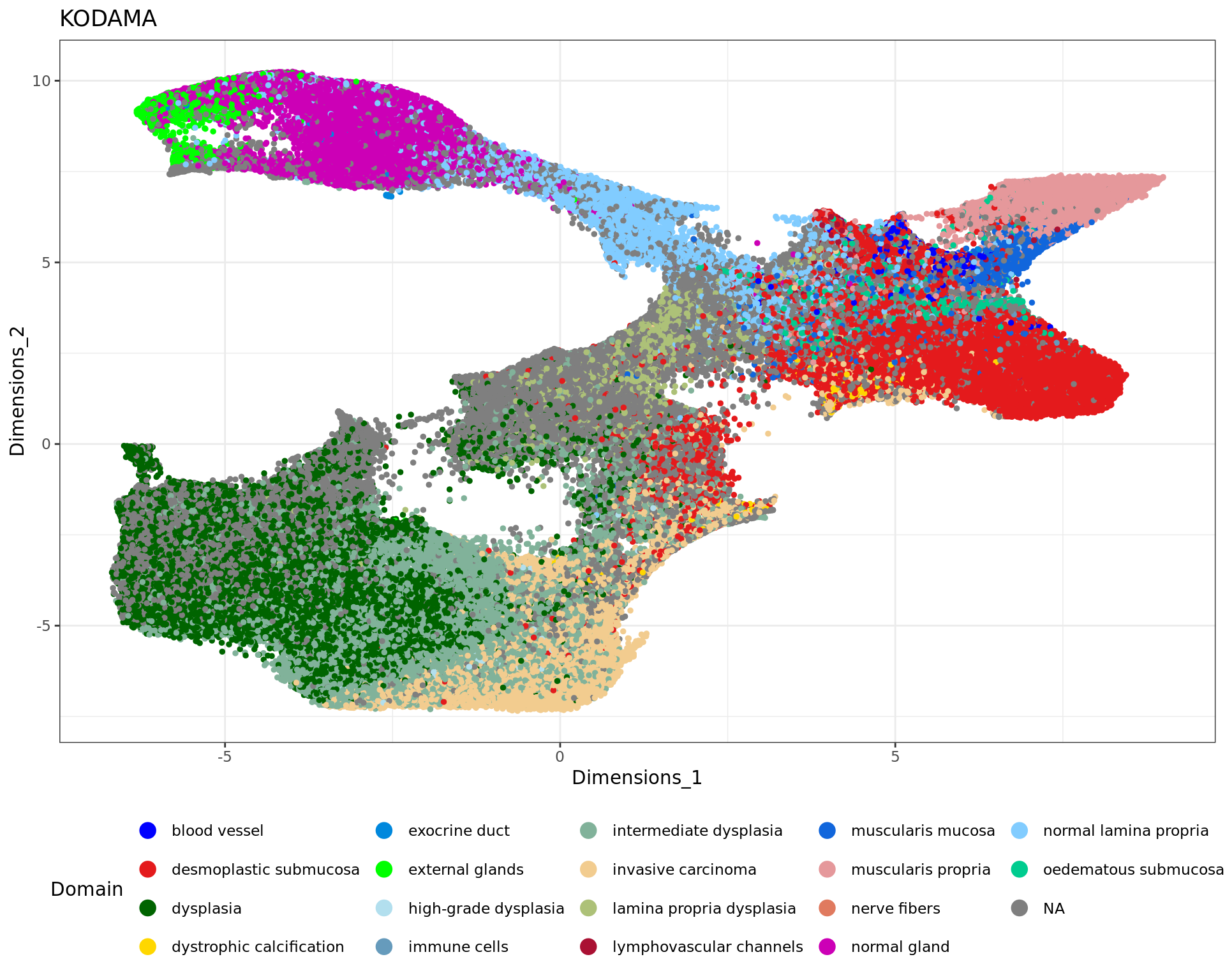
png("output/CRC.png",height = 2000,width = 2000)
plot1
dev.off()
png
2 par(xpd = T, mar = par()$mar + c(0,0,0,7))
plot1=plot(kk_UMAP,cex=0.5,pch=20,col=cols_tissue[labels])
legend(max(kk_UMAP[,1])+0.05*dist(range(kk_UMAP[,1])), max(kk_UMAP[,2]),
levels(labels),
col = cols,
cex = 0.8,
pch=20)
load("data/trajectories_VISIUMHD.RData")
data=sp_obj@assays$Spatial.008um$data[rownames(sp_obj@assays$Spatial.008um$scale.data),]
data=as.matrix(data)Warning in asMethod(object): sparse->dense coercion: allocating vector of size
6.4 GiBdata=t(data)
mm1=new_trajectory (kk_UMAP,data = data,trace=tra1$xy)
mm2=new_trajectory (kk_UMAP,data = data,trace=tra2$xy)
mm3=new_trajectory (kk_UMAP,data = data,trace=tra3$xy)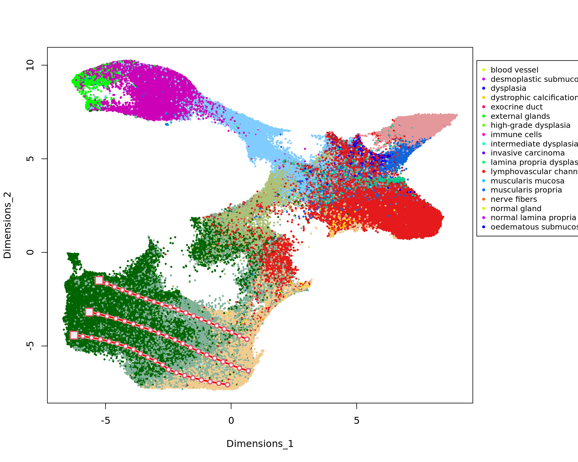
traj=rbind(mm1$trajectory,
           mm2$trajectory,
           mm3$trajectory)
y=rep(1:20,3)
ma=multi_analysis(traj,y,FUN="correlation.test",method="spearman")
ma=ma[order(as.numeric(ma$`p-value`)),]
colnames(ma)=c("Feature ","rho ","p-value ","FDR ")knitr::kable(ma[1:30,],row.names=FALSE)| Feature | rho | p-value | FDR |
|---|---|---|---|
| LCN2 | -0.90 | 1.22e-22 | 1.50e-19 |
| CXCL2 | -0.78 | 2.82e-13 | 1.48e-10 |
| CXCL3 | -0.78 | 3.62e-13 | 1.48e-10 |
| PI3 | -0.77 | 1.04e-12 | 3.21e-10 |
| GPX2 | -0.76 | 1.57e-12 | 3.85e-10 |
| SOD2 | -0.72 | 5.82e-11 | 1.19e-08 |
| CCL20 | -0.72 | 9.89e-11 | 1.74e-08 |
| MUC1 | -0.68 | 2.03e-09 | 3.12e-07 |
| TRIM31 | -0.66 | 8.18e-09 | 1.12e-06 |
| BACE2 | -0.65 | 1.46e-08 | 1.79e-06 |
| SPINK1 | -0.65 | 2.39e-08 | 2.67e-06 |
| CXCL1 | -0.64 | 5.02e-08 | 5.15e-06 |
| CDC25B | -0.63 | 6.51e-08 | 6.16e-06 |
| S100P | -0.60 | 4.58e-07 | 4.03e-05 |
| ID1 | -0.59 | 6.07e-07 | 4.98e-05 |
| LRATD1 | -0.58 | 1.38e-06 | 1.06e-04 |
| FXYD3 | -0.57 | 1.89e-06 | 1.37e-04 |
| SELENBP1 | -0.57 | 2.29e-06 | 1.56e-04 |
| NAMPT | -0.57 | 2.5e-06 | 1.62e-04 |
| LGR5 | 0.56 | 2.72e-06 | 1.67e-04 |
| AREG | -0.56 | 3.32e-06 | 1.94e-04 |
| CDC20 | -0.56 | 3.69e-06 | 2.07e-04 |
| STMN3 | -0.56 | 3.95e-06 | 2.11e-04 |
| NCOA7 | -0.55 | 6.49e-06 | 3.32e-04 |
| S100A9 | -0.54 | 7.43e-06 | 3.65e-04 |
| DNTTIP1 | -0.54 | 8.47e-06 | 4.01e-04 |
| PTP4A3 | -0.53 | 1.22e-05 | 5.55e-04 |
| UBE2C | -0.53 | 1.28e-05 | 5.55e-04 |
| CFB | -0.53 | 1.31e-05 | 5.55e-04 |
| NOS2 | -0.52 | 1.71e-05 | 7.00e-04 |
miRseq Analysis:
Analysing miRseq Gene Expression Data from a Colerectal Adenocarcinoma Cohort:
# install.packages("readxl")
library(readxl)
Prepare Clinical Data:
# Read in Clinical Data:
coad=read.csv("../TCGA/COAD/COAD.clin.merged.picked.txt",sep="\t",check.names = FALSE, row.names = 1)

coad <- as.data.frame(coad)

# Clean column names: replace dots with dashes & convert to uppercase
colnames(coad) = toupper(colnames(coad))

 # Transpose the dataframe so that rows become columns and vice versa
coad = t(coad)
Prepare miRNA-seq expression data:
# Read RNA-seq expression data:
r = read.csv("../TCGA/COAD/COAD.rnaseqv2__illuminahiseq_rnaseqv2__unc_edu__Level_3__RSEM_genes_normalized__data.data.txt", sep = "\t", check.names = FALSE, row.names = 1)
# Remove the first row:
r = r[-1,]
# Convert expression data to numeric matrix format
temp = matrix(as.numeric(as.matrix(r)), ncol=ncol(r))
colnames(temp) = colnames(r)
rownames(temp) = rownames(r)
RNA = temp

# Transpose the matrix so that genes are rows and samples are columns
RNA = t(RNA)
Extract patient and tissue information from column names:
tcgaID = list()
 # Extract sample ID
tcgaID$sample.ID <- substr(colnames(r), 1, 16)
# Extract patient ID
tcgaID$patient <- substr(colnames(r), 1, 12)
# Extract tissue type
tcgaID$tissue <- substr(colnames(r), 14, 16)

tcgaID = as.data.frame(tcgaID)
Select Primary Solid Tumor tissue data (“01A”):
sel=tcgaID$tissue == "01A"
tcgaID.sel = tcgaID[sel, ]

# Subset the RNA expression data to match selected samples
RNA.sel = RNA[sel, ]
Intersect patient IDs between clinical and RNA data:
sel = intersect(tcgaID.sel$patient, rownames(coad))
# Subset the clinical data to include only selected patients:
coad.sel = coad[sel, ]
# Assign patient IDs as row names to the RNA data:
rownames(RNA.sel) = tcgaID.sel$patient
# Subset the RNA data to include only selected patients
RNA.sel = RNA.sel[sel, ]
Prepare labels for pathology stages:
Classify stages
t1,t2, &t3as “low”Classify stages
t4,t4a, &t4bas “high”Convert any
tisstages toNA
labelsTCGA = coad.sel[, "pathology_T_stage"]
labelsTCGA[labelsTCGA %in% c("t1", "t2", "t3", "tis")] = "low"
labelsTCGA[labelsTCGA %in% c("t4", "t4a", "t4b")] = "high"
Log Transform the expression data for our selected gene
CXCL2:
CXCL2 <- log(1 + RNA.sel[, "CXCL2|2920"])
LCN2 <- log(1 + RNA.sel[,"LCN2|3934" ])
Boxplot to visualize the distribution of log transformed gene expression by pathology stage:
colors=c("#0073c2bb","#efc000bb","#868686bb","#cd534cbb","#7aabdcbb","#003c67bb")

library(ggpubr)
df=data.frame(variable=CXCL2,labels=labelsTCGA)

my_comparisons=list()
my_comparisons[[1]]=c(1,2)

Nplot1=ggboxplot(df, x = "labels", y = "variable",fill="labels",
                 width = 0.8,
                 palette=colors,
                 add = "jitter",
                 add.params = list(size = 2, jitter = 0.2,fill=3, shape=10))+
  ylab("CXCL2 gene expression (FPKM)")+ xlab("")+
  stat_compare_means(comparisons = my_comparisons,method="wilcox.test")

Nplot1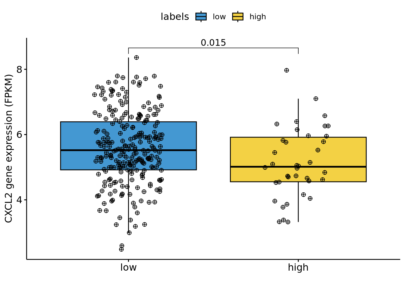
xy2=xy
xy2[,1]=xy[,2]
xy2[,2]=-xy[,1]
plot(xy2,col=cols_tissue[labels],pch=20,cex=0.5)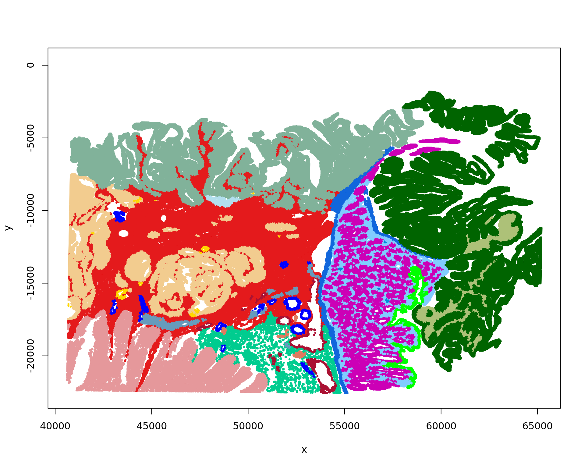
df <- data.frame(xy2, tissue=labels)
plot2 = ggplot(df, aes(x, y, color = tissue)) +labs(title="KODAMA") +
  geom_point(size = 1) +
  theme_bw() + theme(legend.position = "bottom")+
  scale_color_manual("Domain", values = cols_tissue) +
  guides(color = guide_legend(nrow = 4,
                              override.aes = list(size = 4)))
plot2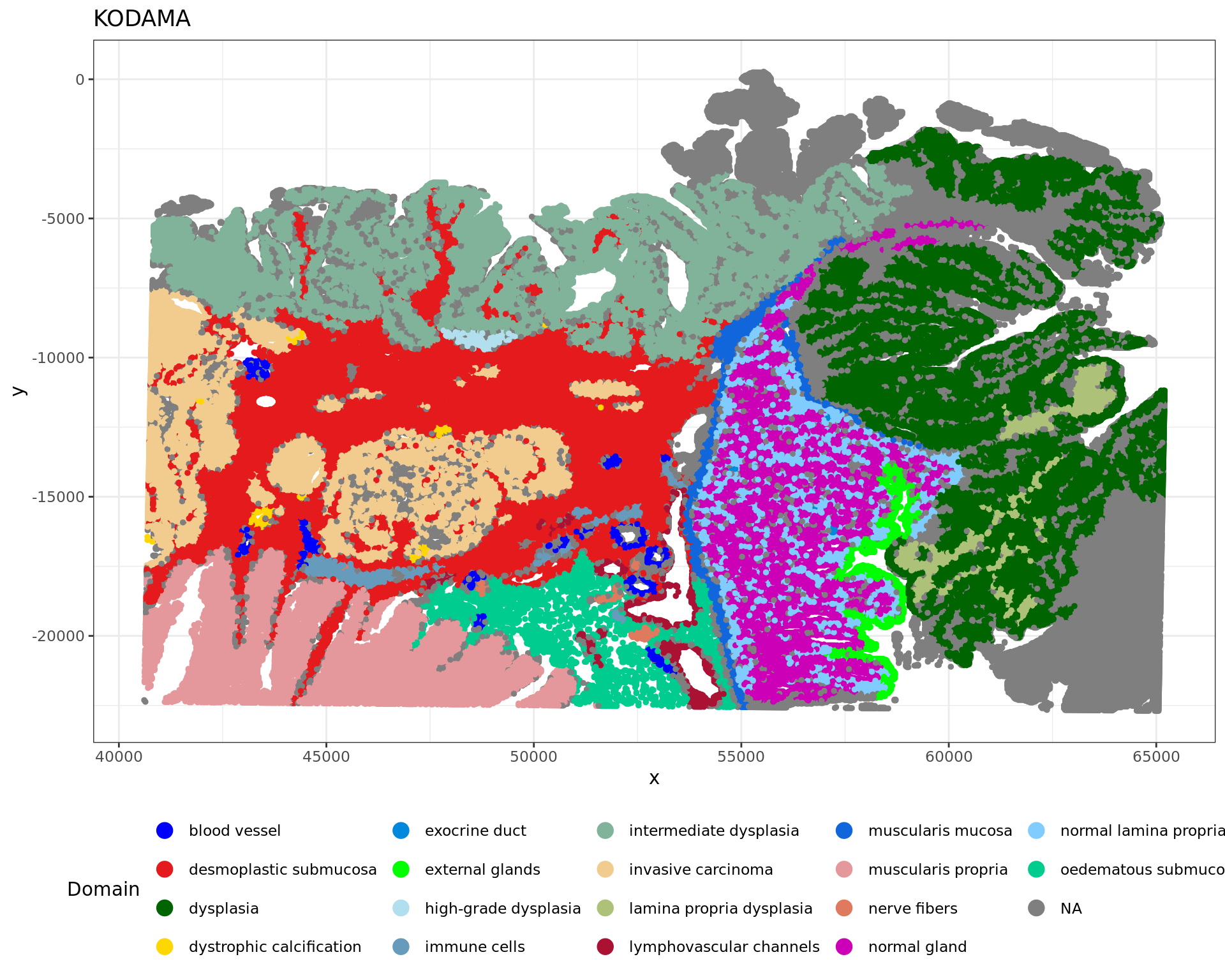
png("output/CRC2.png",height = 2000,width = 2000)
plot2
dev.off()

sel_desmoplastic_submucosa=which(labels=="desmoplastic submucosa")
kk_desmoplastic_submucosa=kk_UMAP[sel_desmoplastic_submucosa,]
xy_desmoplastic_submucosa=xy2[sel_desmoplastic_submucosa,]


g <- bluster::makeSNNGraph(as.matrix(kk_desmoplastic_submucosa), k = 20)
g_walk <- igraph::cluster_louvain(g,resolution = 0.005)
clu = g_walk$membership
names(clu)=rownames(kk_desmoplastic_submucosa)


df <- data.frame(kk_desmoplastic_submucosa[,1:2], tissue=as.factor(clu))
plot3 = ggplot(df, aes(Dimensions_1, Dimensions_2, color = tissue)) +labs(title="KODAMA") +
  geom_point(size = 1) +
  theme_bw() + theme(legend.position = "bottom")+
  scale_color_manual("Domain", values = cols_tissue) +
  guides(color = guide_legend(nrow = 4,
                              override.aes = list(size = 4)))
plot3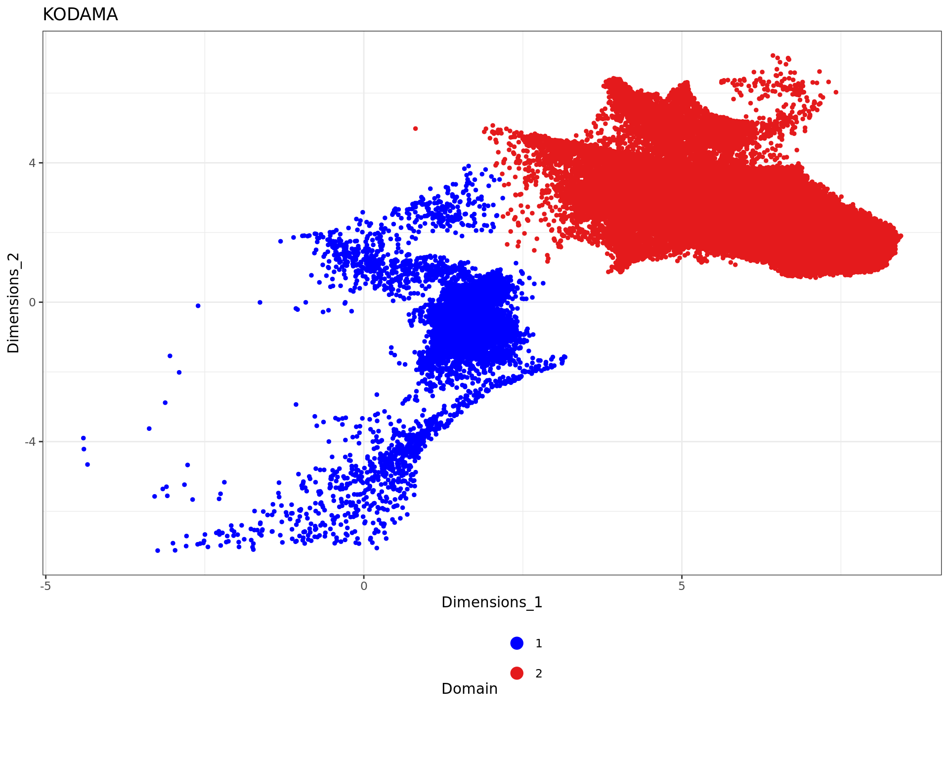
png("output/CRC7.png",height = 2000,width = 2000)
plot3
dev.off()


df <- data.frame(xy_desmoplastic_submucosa, tissue=as.factor(clu))
plot4 = ggplot(df, aes(x, y, color = tissue)) +labs(title="KODAMA") +
  geom_point(size = 1) +
  theme_bw() + theme(legend.position = "bottom")+
  scale_color_manual("Domain", values = cols_tissue) +
  guides(color = guide_legend(nrow = 4,
                              override.aes = list(size = 4)))
plot4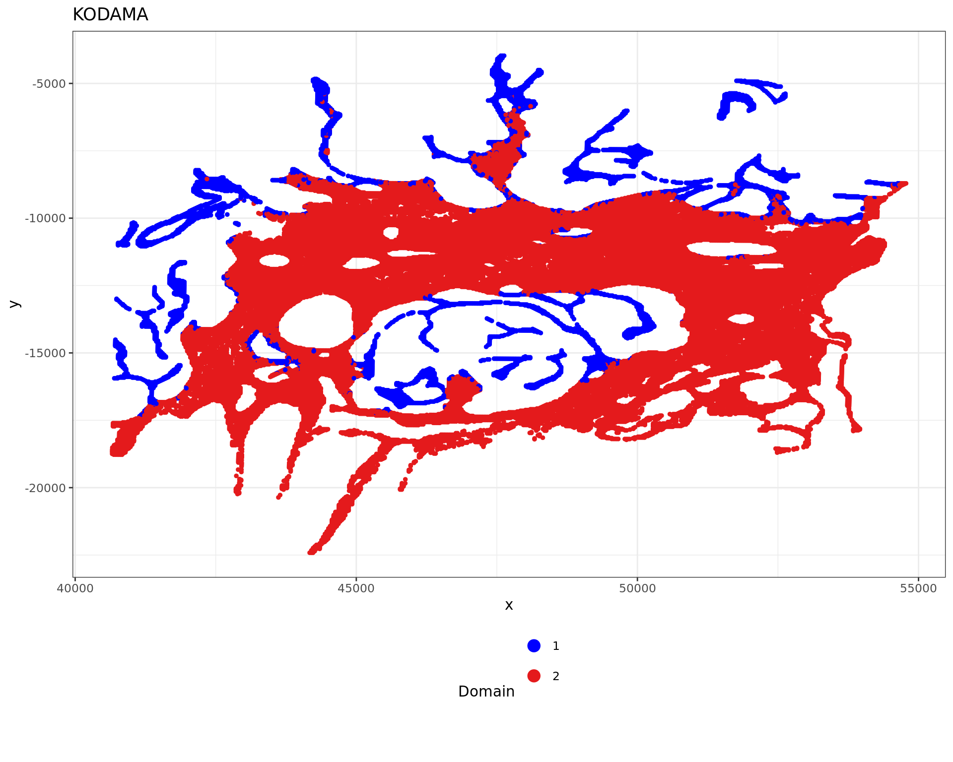
png("output/CRC8.png",height = 2000,width = 2000)
plot4
dev.off()


sel_desmoplastic_submucosa_selected=names(which(clu==names(which.max(table(clu)))))
kk_desmoplastic_submucosa_selected=kk_UMAP[sel_desmoplastic_submucosa_selected,]
xy_desmoplastic_submucosa_selected=xy2[sel_desmoplastic_submucosa_selected,]
data_desmoplastic_submucosa_selected=data[sel_desmoplastic_submucosa_selected,]
data_desmoplastic_submucosa_selected=data_desmoplastic_submucosa_selected[,-which(colMeans(data_desmoplastic_submucosa_selected==0)>0.95)]

sel_invasive_carcinoma=which(labels=="invasive carcinoma" | labels=="intermediate dysplasia")
kk_invasive_carcinoma=kk_UMAP[sel_invasive_carcinoma,]
xy_invasive_carcinoma=xy2[sel_invasive_carcinoma,]

knn=Rnanoflann::nn(xy_invasive_carcinoma,xy_desmoplastic_submucosa_selected,1)

y=knn$distances[,1]


ma=multi_analysis(data_desmoplastic_submucosa_selected,y,FUN="correlation.test",method="spearman")
ma=ma[order(abs(as.numeric(ma$rho)),decreasing = TRUE),]
colnames(ma)=c("Feature   ","rho   ","p-value   ","FDR   ")


# 2) Define custom intervals
break_points <-c(quantile(y,probs=c(seq(0,1,0.005))))

# 3) Convert continuous data to intervals
distance_binned <- cut(y, breaks = break_points)

gene_binned=apply(data_desmoplastic_submucosa_selected,2,function(x)  tapply(x,distance_binned,mean))
break_points=break_points[-length(break_points)]

ma=multi_analysis(gene_binned,break_points,FUN="correlation.test",method="MINE")
ma=ma[order(as.numeric(ma$MIC),decreasing = TRUE),]
ma[1:10,]
rownames(ma)=ma[,"Feature"]
#plot(knn$distances,PMdata[,3])

zmax=NULL
for(i in 1:ncol(gene_binned)){
 df=data.frame(x=break_points,y=gene_binned[,i])
 ll=loess(y~x,data = df,span = 0.3)
 z=predict(ll,newdata = data.frame(x=break_points))
 zmax[i]=break_points[which.max(z)]
# points(break_points,z,type="l",col=2)
}
genes=colnames(gene_binned)
names(zmax)=genes


plot(log(1+zmax[genes]),ma[genes,]$MIC,cex=0.2)
text(log(1+zmax[genes]),ma[genes,]$MIC,labels=genes,cex=0.7)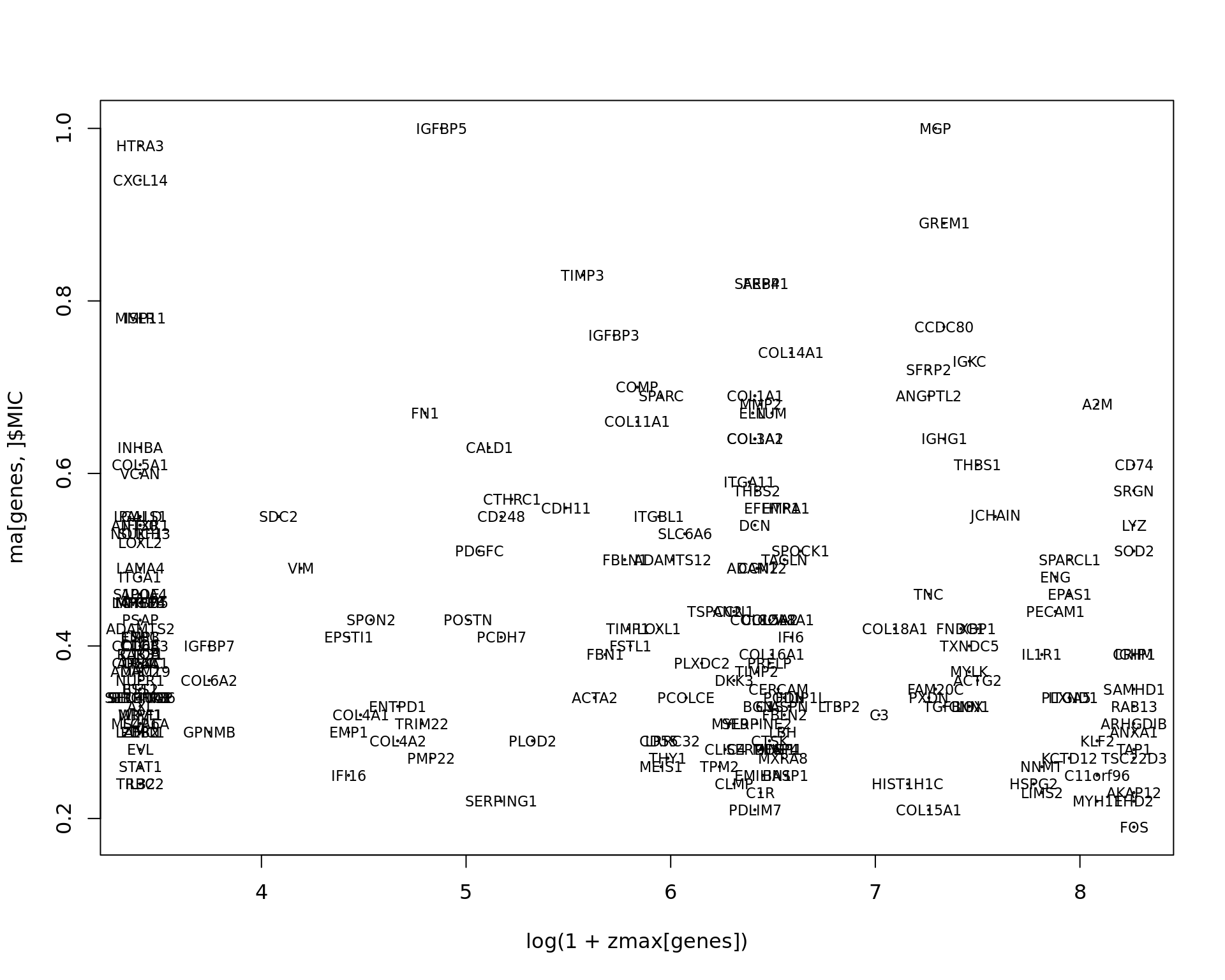
plot(log(1+break_points),gene_binned[,1],ylim=c(0,1),type="n")
 df=data.frame(x=break_points,
               HTRA3=gene_binned[,"HTRA3"],
               IGFBP5=gene_binned[,"IGFBP5"],
               CXCL14=gene_binned[,"CXCL14"],
               MMP11=gene_binned[,"MMP11"],
               TIMP3=gene_binned[,"TIMP3"],
               MGP=gene_binned[,"MGP"])

 ll=loess(IGFBP5~x,data = df,span = 0.3)
 IGFBP5=predict(ll,newdata = data.frame(x=break_points))

 ll=loess(CXCL14~x,data = df,span = 0.3)
 CXCL14=predict(ll,newdata = data.frame(x=break_points))

 ll=loess(MMP11~x,data = df,span = 0.3)
 MMP11=predict(ll,newdata = data.frame(x=break_points))

 ll=loess(TIMP3~x,data = df,span = 0.3)
 TIMP3=predict(ll,newdata = data.frame(x=break_points))

 ll=loess(HTRA3~x,data = df,span = 0.3)
 HTRA3=predict(ll,newdata = data.frame(x=break_points))

 ll=loess(MGP~x,data = df,span = 0.3)
 MGP=predict(ll,newdata = data.frame(x=break_points))
 points(log(1+break_points),HTRA3/max(HTRA3),type="l",col=2,lwd=3)
 points(log(1+break_points),IGFBP5/max(IGFBP5),type="l",col=3,lwd=3)
 points(log(1+break_points),CXCL14/max(CXCL14),type="l",col=4,lwd=3)
 points(log(1+break_points),MMP11/max(MMP11),type="l",col=5,lwd=3)
 points(log(1+break_points),TIMP3/max(TIMP3),type="l",col=6,lwd=3)
 points(log(1+break_points),MGP/max(MGP),type="l",col=7,lwd=3)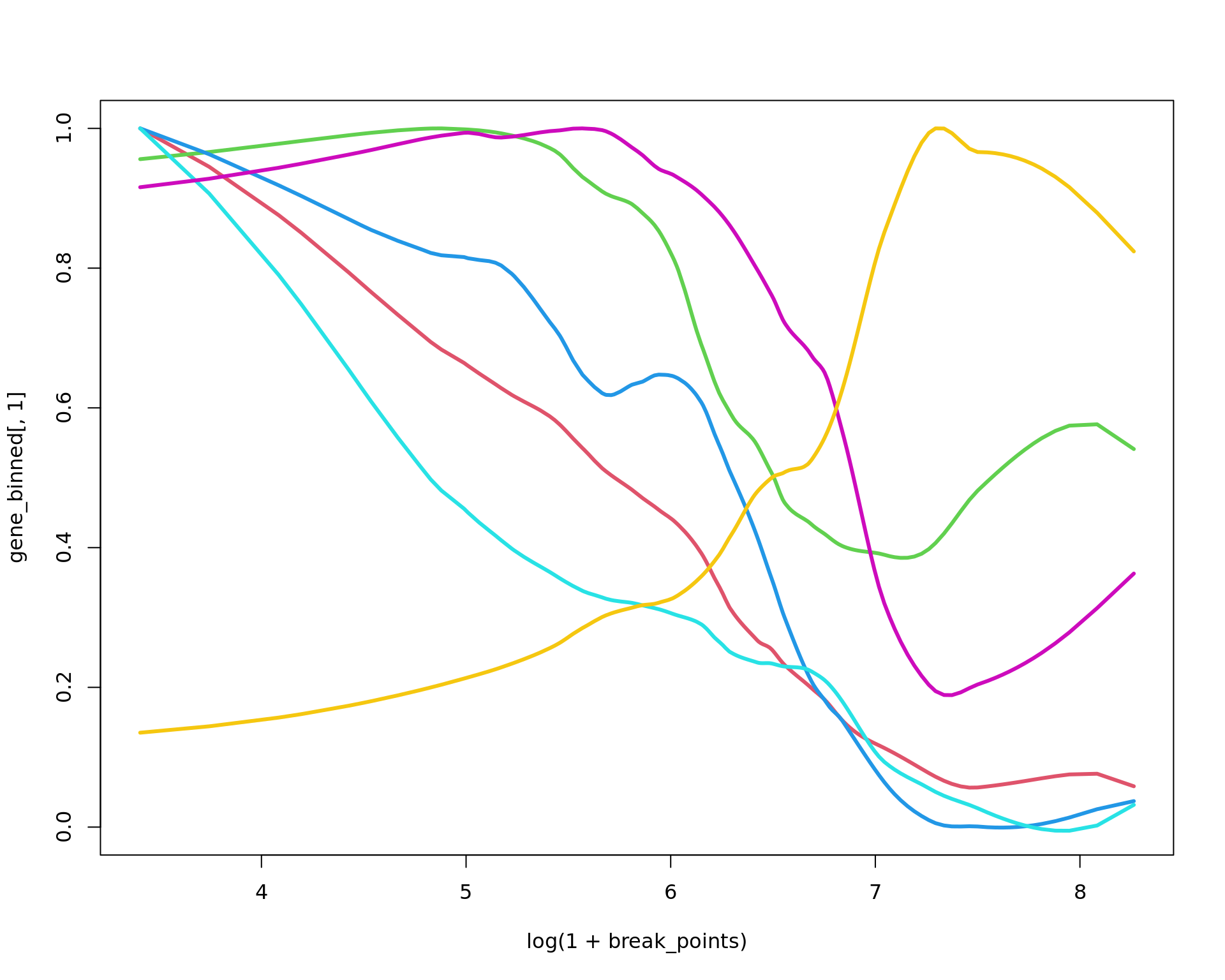
knitr::kable(ma[1:30,],row.names=FALSE)| Feature | MIC | p-value | FDR |
|---|---|---|---|
| IGFBP5 | 1.00 | 6.8e-241 | 3.52e-239 |
| MGP | 1.00 | 1.79e-277 | 1.85e-275 |
| HTRA3 | 0.98 | 0e+00 | 0.00e+00 |
| CXCL14 | 0.94 | 1.11e-256 | 7.68e-255 |
| GREM1 | 0.89 | 5.49e-180 | 2.27e-178 |
| TIMP3 | 0.83 | 3.75e-142 | 9.71e-141 |
| SFRP4 | 0.82 | 1.09e-139 | 2.50e-138 |
| AEBP1 | 0.82 | 2.46e-139 | 5.09e-138 |
| ISLR | 0.78 | 9.88e-115 | 1.46e-113 |
| MMP11 | 0.78 | 2.86e-143 | 8.46e-142 |
| CCDC80 | 0.77 | 1.42e-92 | 1.47e-91 |
| IGFBP3 | 0.76 | 7.7e-145 | 2.66e-143 |
| COL14A1 | 0.74 | 1.6e-95 | 1.84e-94 |
| IGKC | 0.73 | 1.5e-112 | 2.07e-111 |
| SFRP2 | 0.72 | 2.34e-73 | 1.80e-72 |
| COMP | 0.70 | 3.01e-87 | 2.71e-86 |
| SPARC | 0.69 | 1.74e-96 | 2.11e-95 |
| ANGPTL2 | 0.69 | 2.66e-100 | 3.44e-99 |
| COL1A1 | 0.69 | 1.88e-116 | 3.24e-115 |
| A2M | 0.68 | 5.44e-95 | 5.93e-94 |
| MMP2 | 0.68 | 3.48e-92 | 3.43e-91 |
| FN1 | 0.67 | 7.81e-72 | 5.58e-71 |
| ELN | 0.67 | 4.9e-115 | 7.80e-114 |
| LUM | 0.67 | 2.02e-81 | 1.74e-80 |
| COL11A1 | 0.66 | 8e-90 | 7.53e-89 |
| COL3A1 | 0.64 | 5.02e-72 | 3.71e-71 |
| COL1A2 | 0.64 | 3.94e-55 | 2.26e-54 |
| IGHG1 | 0.64 | 4.41e-80 | 3.65e-79 |
| INHBA | 0.63 | 2.2e-61 | 1.42e-60 |
| CALD1 | 0.63 | 1.44e-130 | 2.71e-129 |
sessionInfo()R version 4.4.2 (2024-10-31)
Platform: x86_64-pc-linux-gnu
Running under: Ubuntu 20.04.6 LTS
Matrix products: default
BLAS: /usr/lib/x86_64-linux-gnu/blas/libblas.so.3.9.0
LAPACK: /usr/lib/x86_64-linux-gnu/lapack/liblapack.so.3.9.0
locale:
[1] LC_CTYPE=en_US.UTF-8 LC_NUMERIC=C
[3] LC_TIME=en_US.UTF-8 LC_COLLATE=en_US.UTF-8
[5] LC_MONETARY=en_US.UTF-8 LC_MESSAGES=en_US.UTF-8
[7] LC_PAPER=en_US.UTF-8 LC_NAME=C
[9] LC_ADDRESS=C LC_TELEPHONE=C
[11] LC_MEASUREMENT=en_US.UTF-8 LC_IDENTIFICATION=C
time zone: Etc/UTC
tzcode source: system (glibc)
attached base packages:
[1] parallel stats graphics grDevices utils datasets methods
[8] base
other attached packages:
[1] ggpubr_0.6.0 readxl_1.4.3 bigmemory_4.6.4 KODAMAextra_1.2
[5] e1071_1.7-16 doParallel_1.0.17 iterators_1.0.14 foreach_1.5.2
[9] KODAMA_3.0 Matrix_1.7-1 umap_0.2.10.0 Rtsne_0.17
[13] minerva_1.5.10 Seurat_5.1.0 SeuratObject_5.0.2 sp_2.1-4
[17] dplyr_1.1.4 patchwork_1.3.0 ggplot2_3.5.1 workflowr_1.7.1
loaded via a namespace (and not attached):
[1] RcppAnnoy_0.0.22 splines_4.4.2 later_1.4.0
[4] tibble_3.2.1 cellranger_1.1.0 polyclip_1.10-7
[7] fastDummies_1.7.4 lifecycle_1.0.4 rstatix_0.7.2
[10] tcltk_4.4.2 rprojroot_2.0.4 globals_0.16.3
[13] processx_3.8.4 Rnanoflann_0.0.3 lattice_0.22-6
[16] hdf5r_1.3.11 MASS_7.3-61 backports_1.5.0
[19] magrittr_2.0.3 plotly_4.10.4 sass_0.4.9
[22] rmarkdown_2.29 jquerylib_0.1.4 yaml_2.3.10
[25] httpuv_1.6.15 sctransform_0.4.1 spam_2.11-0
[28] askpass_1.2.1 spatstat.sparse_3.1-0 reticulate_1.38.0
[31] cowplot_1.1.3 pbapply_1.7-2 RColorBrewer_1.1-3
[34] abind_1.4-8 purrr_1.0.2 BiocGenerics_0.50.0
[37] misc3d_0.9-1 git2r_0.33.0 S4Vectors_0.42.1
[40] ggrepel_0.9.6 irlba_2.3.5.1 listenv_0.9.1
[43] spatstat.utils_3.1-2 goftest_1.2-3 RSpectra_0.16-2
[46] spatstat.random_3.3-2 fitdistrplus_1.2-2 parallelly_1.41.0
[49] leiden_0.4.3.1 codetools_0.2-20 tidyselect_1.2.1
[52] farver_2.1.2 stats4_4.4.2 matrixStats_1.4.1
[55] spatstat.explore_3.3-3 jsonlite_1.8.9 BiocNeighbors_1.22.0
[58] Formula_1.2-5 progressr_0.14.0 ggridges_0.5.6
[61] survival_3.8-3 tools_4.4.2 ica_1.0-3
[64] Rcpp_1.0.13-1 glue_1.8.0 gridExtra_2.3
[67] xfun_0.49 withr_3.0.1 fastmap_1.2.0
[70] bluster_1.14.0 fansi_1.0.6 openssl_2.2.2
[73] callr_3.7.6 digest_0.6.37 R6_2.5.1
[76] mime_0.12 colorspace_2.1-1 scattermore_1.2
[79] tensor_1.5 spatstat.data_3.1-4 utf8_1.2.4
[82] tidyr_1.3.1 generics_0.1.3 data.table_1.15.4
[85] class_7.3-23 httr_1.4.7 htmlwidgets_1.6.4
[88] whisker_0.4.1 uwot_0.2.2 pkgconfig_2.0.3
[91] gtable_0.3.5 lmtest_0.9-40 htmltools_0.5.8.1
[94] carData_3.0-5 dotCall64_1.2 scales_1.3.0
[97] png_0.1-8 spatstat.univar_3.1-1 bigmemory.sri_0.1.8
[100] knitr_1.49 rstudioapi_0.17.1 reshape2_1.4.4
[103] uuid_1.2-1 nlme_3.1-166 proxy_0.4-27
[106] cachem_1.1.0 zoo_1.8-12 stringr_1.5.1
[109] KernSmooth_2.23-26 miniUI_0.1.1.1 vipor_0.4.7
[112] arrow_16.1.0 ggrastr_1.0.2 pillar_1.9.0
[115] grid_4.4.2 vctrs_0.6.5 RANN_2.6.2
[118] promises_1.3.2 car_3.1-3 xtable_1.8-4
[121] cluster_2.1.8 beeswarm_0.4.0 evaluate_1.0.1
[124] cli_3.6.3 compiler_4.4.2 rlang_1.1.4
[127] future.apply_1.11.3 ggsignif_0.6.4 labeling_0.4.3
[130] ps_1.8.1 getPass_0.2-4 plyr_1.8.9
[133] fs_1.6.5 ggbeeswarm_0.7.2 stringi_1.8.4
[136] BiocParallel_1.38.0 viridisLite_0.4.2 deldir_2.0-4
[139] assertthat_0.2.1 munsell_0.5.1 lazyeval_0.2.2
[142] spatstat.geom_3.3-4 RcppHNSW_0.6.0 bit64_4.5.2
[145] future_1.34.0 shiny_1.10.0 ROCR_1.0-11
[148] broom_1.0.7 igraph_2.0.3 bslib_0.8.0
[151] bit_4.5.0.1