DLPFC
Last updated: 2024-10-16
Checks: 7 0
Knit directory: KODAMA-Analysis/
This reproducible R Markdown analysis was created with workflowr (version 1.7.1). The Checks tab describes the reproducibility checks that were applied when the results were created. The Past versions tab lists the development history.
Great! Since the R Markdown file has been committed to the Git repository, you know the exact version of the code that produced these results.
Great job! The global environment was empty. Objects defined in the global environment can affect the analysis in your R Markdown file in unknown ways. For reproduciblity it’s best to always run the code in an empty environment.
The command set.seed(20240618) was run prior to running
the code in the R Markdown file. Setting a seed ensures that any results
that rely on randomness, e.g. subsampling or permutations, are
reproducible.
Great job! Recording the operating system, R version, and package versions is critical for reproducibility.
Nice! There were no cached chunks for this analysis, so you can be confident that you successfully produced the results during this run.
Great job! Using relative paths to the files within your workflowr project makes it easier to run your code on other machines.
Great! You are using Git for version control. Tracking code development and connecting the code version to the results is critical for reproducibility.
The results in this page were generated with repository version df98881. See the Past versions tab to see a history of the changes made to the R Markdown and HTML files.
Note that you need to be careful to ensure that all relevant files for
the analysis have been committed to Git prior to generating the results
(you can use wflow_publish or
wflow_git_commit). workflowr only checks the R Markdown
file, but you know if there are other scripts or data files that it
depends on. Below is the status of the Git repository when the results
were generated:
Ignored files:
    Ignored:    .RData
    Ignored:    .Rhistory
    Ignored:    .Rproj.user/
    Ignored:    analysis/figure/

Untracked files:
    Untracked:  KODAMA.svg
    Untracked:  code/Acinar_Cell_Carcinoma.ipynb
    Untracked:  code/Adenocarcinoma.ipynb
    Untracked:  code/Adjacent_normal_section.ipynb
    Untracked:  code/DLFPC_preprocessing.R
    Untracked:  code/DLPFC - BANKSY.R
    Untracked:  code/DLPFC - BASS.R
    Untracked:  code/DLPFC - BAYESPACE.R
    Untracked:  code/DLPFC - Nonspatial.R
    Untracked:  code/DLPFC - PRECAST.R
    Untracked:  code/DLPFC_comparison.R
    Untracked:  code/VisiumHD-CRC.ipynb
    Untracked:  data/DLFPC-Br5292-input.RData
    Untracked:  data/DLFPC-Br5595-input.RData
    Untracked:  data/DLFPC-Br8100-input.RData
    Untracked:  data/DLPFC-general.RData
    Untracked:  data/spots_classification_ALL.csv
    Untracked:  data/trajectories.RData
    Untracked:  data/trajectories_VISIUMHD.RData
    Untracked:  output/BANSKY-results.RData
    Untracked:  output/BASS-results.RData
    Untracked:  output/CRC-image.RData
    Untracked:  output/CRC-image2.RData
    Untracked:  output/DLFPC-All.RData
    Untracked:  output/DLFPC-Br5292.RData
    Untracked:  output/DLFPC-Br5595.RData
    Untracked:  output/DLFPC-Br8100.RData
    Untracked:  output/KODAMA-results.RData
    Untracked:  output/MERFISH.RData
    Untracked:  output/Nonspatial-results.RData
    Untracked:  output/Prostate.RData
    Untracked:  output/VisiumHD3.RData
    Untracked:  output/image.RData

Unstaged changes:
    Deleted:    analysis/DLPFC-12.Rmd
    Deleted:    analysis/DLPFC-4.Rmd
    Deleted:    analysis/DLPFC1.Rmd
    Deleted:    analysis/DLPFC10.Rmd
    Deleted:    analysis/DLPFC2.Rmd
    Deleted:    analysis/DLPFC3.Rmd
    Deleted:    analysis/DLPFC4.Rmd
    Deleted:    analysis/DLPFC5.Rmd
    Deleted:    analysis/DLPFC6.Rmd
    Deleted:    analysis/DLPFC7.Rmd
    Deleted:    analysis/DLPFC8.Rmd
    Deleted:    analysis/DLPFC9.Rmd
    Modified:   analysis/Giotto.Rmd
    Deleted:    analysis/STARmap.Rmd
    Modified:   analysis/VisiumHD.Rmd
Note that any generated files, e.g. HTML, png, CSS, etc., are not included in this status report because it is ok for generated content to have uncommitted changes.
These are the previous versions of the repository in which changes were
made to the R Markdown (analysis/DLPFC.Rmd) and HTML
(docs/DLPFC.html) files. If you’ve configured a remote Git
repository (see ?wflow_git_remote), click on the hyperlinks
in the table below to view the files as they were in that past version.
| File | Version | Author | Date | Message |
|---|---|---|---|---|
| Rmd | df98881 | Stefano Cacciatore | 2024-10-16 | Start my new project |
| Rmd | 47b0163 | Stefano Cacciatore | 2024-10-15 | Start my new project |
| html | fd8d092 | Stefano Cacciatore | 2024-10-15 | Build site. |
| Rmd | e31e3e8 | Stefano Cacciatore | 2024-10-15 | Start my new project |
| html | 1edc32b | Stefano Cacciatore | 2024-10-11 | Build site. |
| Rmd | eaad1a0 | Stefano Cacciatore | 2024-10-11 | Start my new project |
| html | c9d54ee | Stefano Cacciatore | 2024-10-11 | Build site. |
| Rmd | fa049de | Stefano Cacciatore | 2024-10-11 | Start my new project |
| Rmd | 454b8fc | Stefano Cacciatore | 2024-10-11 | Start my new project |
| html | 1352d91 | Stefano Cacciatore | 2024-10-10 | Build site. |
| Rmd | 1b119a0 | Stefano Cacciatore | 2024-10-10 | Start my new project |
| html | 6038af1 | Stefano Cacciatore | 2024-10-09 | Build site. |
| Rmd | d141628 | Stefano Cacciatore | 2024-10-09 | Start my new project |
| html | d1192e9 | Stefano Cacciatore | 2024-08-12 | Build site. |
| html | 3374e66 | Stefano Cacciatore | 2024-08-06 | Build site. |
| html | 35ce733 | Stefano Cacciatore | 2024-08-03 | Build site. |
| Rmd | 06f7055 | Stefano Cacciatore | 2024-08-02 | Start my new project |
| Rmd | 7be8f59 | tkcaccia | 2024-07-15 | updates |
| Rmd | f8ca54a | tkcaccia | 2024-07-14 | update |
| html | f8ca54a | tkcaccia | 2024-07-14 | update |
| html | 3ea09a6 | GitHub | 2024-07-08 | Update DLPFC.html |
| html | 93915d8 | GitHub | 2024-07-04 | Update DLPFC.html |
| html | ee4ee17 | GitHub | 2024-06-19 | Add files via upload |
| Rmd | 615fc05 | GitHub | 2024-06-19 | Add files via upload |
Introduction
Here, we apply KODAMA to analyze the human dorsolateral prefrontal cortex (DLPFC) data by 10x Visium from Maynard et al., 2021. The links to download the raw data and H&E full resolution images can be found in the LieberInstitute/spatialLIBD github page.
Loading the required libraries
library("nnSVG")
library("scater")
library("scran")
library("scry")
library("SPARK")
library("harmony")
library("Seurat")
library("spatialLIBD")
library("KODAMAextra")
library("mclust")
library("slingshot")
library("irlba")
Download the dataset
spe <- fetch_data(type = 'spe')Extract the metadata information
n.cores=40
splitting = 100
spatial.resolution = 0.3
aa_noise=3
gene_number=2000
graph = 20
seed=123


set.seed(seed)
ID=unlist(lapply(strsplit(rownames(colData(spe)),"-"),function(x) x[1]))
samples=colData(spe)$sample_id
rownames(colData(spe))=paste(ID,samples,sep="-")

txtfile=paste(splitting,spatial.resolution,aa_noise,2,gene_number,sep="_")

sample_names=c("151507",
               "151508",
               "151509",
               "151510",
               "151669",
               "151670",
               "151671",
               "151672",
               "151673",
               "151674",
               "151675",
               "151676")
subject_names= c("Br5292","Br5595", "Br8100")
metaData = SingleCellExperiment::colData(spe)
expr = SingleCellExperiment::counts(spe)
sample_names <- paste0("sample_", unique(colData(spe)$sample_id))
sample_names <-  unique(colData(spe)$sample_id)
dim(spe)
[1] 33538 47681# identify mitochondrial genes
is_mito <- grepl("(^MT-)|(^mt-)", rowData(spe)$gene_name)
table(is_mito)is_mito
FALSE TRUE
33525 13 # calculate per-spot QC metrics
spe <- addPerCellQC(spe, subsets = list(mito = is_mito))
# select QC thresholds
qc_lib_size <- colData(spe)$sum < 500
qc_detected <- colData(spe)$detected < 250
qc_mito <- colData(spe)$subsets_mito_percent > 30
qc_cell_count <- colData(spe)$cell_count > 12
# spots to discard
discard <- qc_lib_size | qc_detected | qc_mito | qc_cell_count
table(discard)discard
FALSE TRUE
46653 1028 colData(spe)$discard <- discard
# filter low-quality spots
spe <- spe[, !colData(spe)$discard]
dim(spe)[1] 33538 46653spe <- filter_genes(
spe,
filter_genes_ncounts = 2, #ncounts
filter_genes_pcspots = 0.5,
filter_mito = TRUE
)
dim(spe)[1] 6623 46653sel= !is.na(colData(spe)$layer_guess_reordered)
spe = spe[,sel]
dim(spe)[1] 6623 46318spe <- computeLibraryFactors(spe)
spe <- logNormCounts(spe)Gene selection
The identification of genes that display spatial expression patterns is performed using the SPARKX method (Zhu et al. (2021)). The genes are ranked based on the median value of the logarithm value of the p-value obtained in each slide individually.
top=multi_SPARKX(spe,n.cores=n.cores)Warning in asMethod(object): sparse->dense coercion: allocating vector of size
2.3 GiBdata=as.matrix(t(logcounts(spe)[top[1:gene_number],]))
samples=colData(spe)$sample_id
labels=as.factor(colData(spe)$layer_guess_reordered)
names(labels)=rownames(colData(spe))
subjects=colData(spe)$subjectPatient Br5595
subject_names="Br5595"
nclusters=5

spe_sub <- spe[, colData(spe)$subject ==  subject_names]
 # subjects=colData(spe_sub)$subject
dim(spe_sub)
[1] 6623 14646# spe_sub <- runPCA(spe_sub, 50,subset_row = top[1:gene_number], scale=TRUE)
#pca=reducedDim(spe_sub,type = "PCA")[,1:50]
spe_sub <- spe[, colData(spe)$subject == subject_names]
sel= subjects == subject_names
data_Br5595=data[sel,top[1:gene_number]]
RNA.scaled=scale(data_Br5595)
pca_results <- irlba(A = RNA.scaled, nv = 50)
pca_Br5595 <- pca_results$u %*% diag(pca_results$d)[,1:50]
rownames(pca_Br5595)=rownames(data_Br5595)
colnames(pca_Br5595)=paste("PC",1:50,sep="")
labels=as.factor(colData(spe_sub)$layer_guess_reordered)
names(labels)=rownames(colData(spe_sub))
xy=as.matrix(spatialCoords(spe_sub))
rownames(xy)=rownames(colData(spe_sub))
samples=colData(spe_sub)$sample_id
plot(pca_Br5595, pch=20,col=as.factor(colData(spe_sub)$sample_id))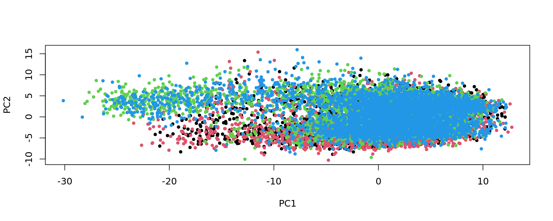
KODAMA analysis
set.seed(seed)
kk=KODAMA.matrix.parallel(pca_Br5595,
                          spatial = xy,
                          samples=samples,
                          FUN= "PLS" ,
                          landmarks = 100000,
                          splitting = splitting,
                          f.par.pls = 50,
                          spatial.resolution = spatial.resolution,
                          n.cores=n.cores,
                          aa_noise=aa_noise,
                          seed = seed)
Calculating Network
Calculating Network spatial
socket cluster with 40 nodes on host 'localhost'
================================================================================
Finished parallel computation
[1] "Calculation of dissimilarity matrix..."
================================================================================print("KODAMA finished")[1] "KODAMA finished"config=umap.defaults
config$n_threads = n.cores
config$n_sgd_threads = "auto"
kk_UMAP=KODAMA.visualization(kk,method="UMAP",config=config)
plot(kk_UMAP,pch=20,col=as.factor(labels))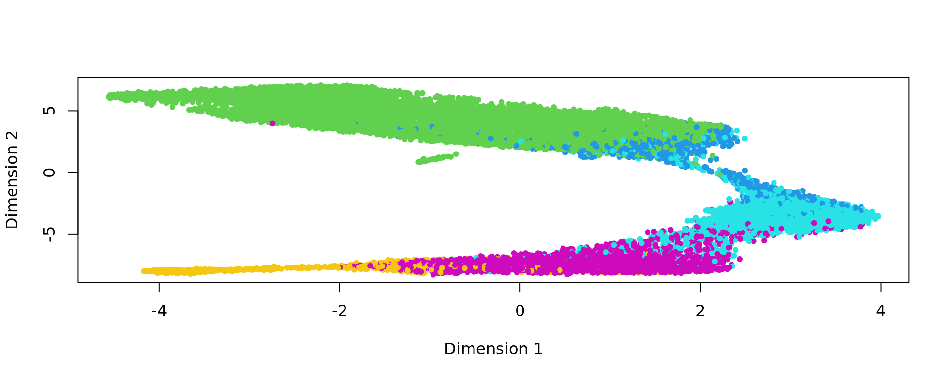
Graph-based clustering
    # Graph-based clustering

g <- bluster::makeSNNGraph(as.matrix(kk_UMAP), k = 20)
g_walk <- igraph::cluster_walktrap(g)
clu <- as.character(igraph::cut_at(g_walk, no = 2))
plot(kk_UMAP,pch=20,col=as.factor(clu))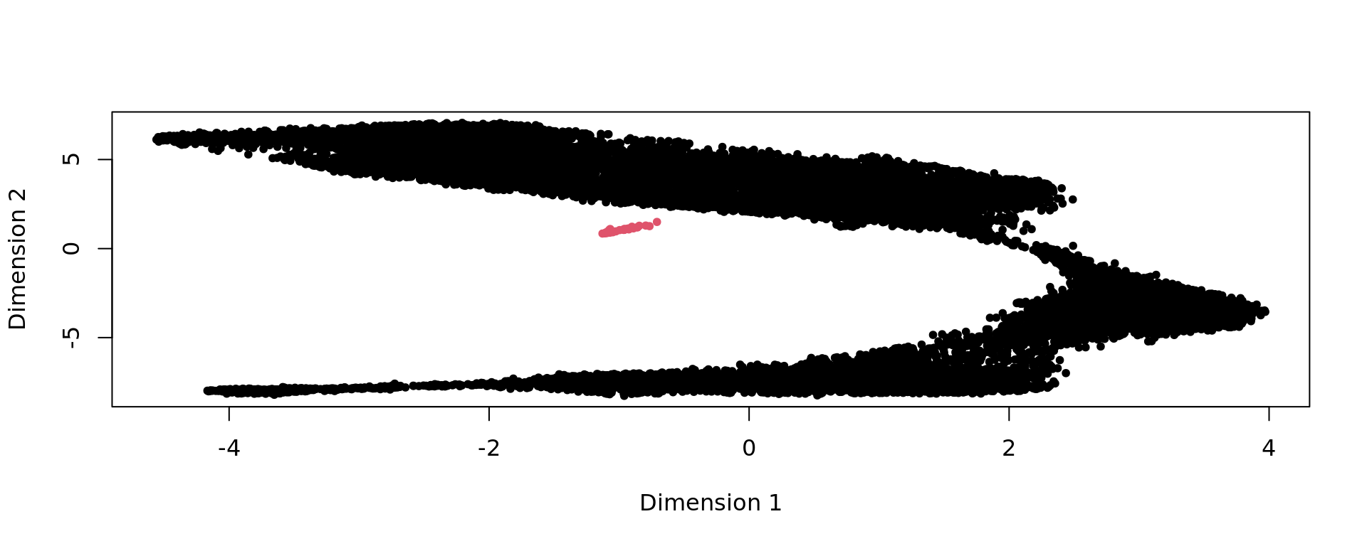
FB=names(which.min(table(clu)))
selFB=clu!=FB

 # kk_UMAP=kk_UMAP[selFB,]
#  labels=labels[selFB]
#  samples=samples[selFB]
#  xy=xy[selFB,]


g <- bluster::makeSNNGraph(as.matrix(kk_UMAP[selFB,]), k = graph)
g_walk <- igraph::cluster_walktrap(g)
clu <- as.character(igraph::cut_at(g_walk, no = nclusters))
plot(kk_UMAP[selFB,],pch=20,col=as.factor(clu))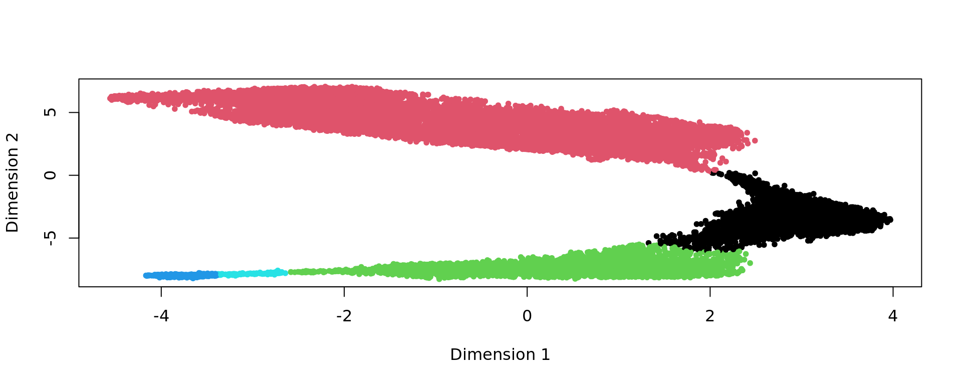
ref=refine_SVM(xy[selFB,],clu,samples[selFB],cost=100)[1] "151669"
[1] "151670"
[1] "151671"
[1] "151672"u=unique(samples[selFB])
for(j in u){
sel=samples[selFB]==j
print(mclust::adjustedRandIndex(labels[selFB][sel],ref[sel]))
}[1] 0.7708206
[1] 0.7696762
[1] 0.8132983
[1] 0.7338236 ###########
cols_cluster <- c("#0000b6", "#81b29a", "#f2cc8f","#e07a5f",
"#cc00b6", "#81ccff", "#33b233")
plot_slide(xy[selFB,],samples[selFB],ref,col=cols_cluster)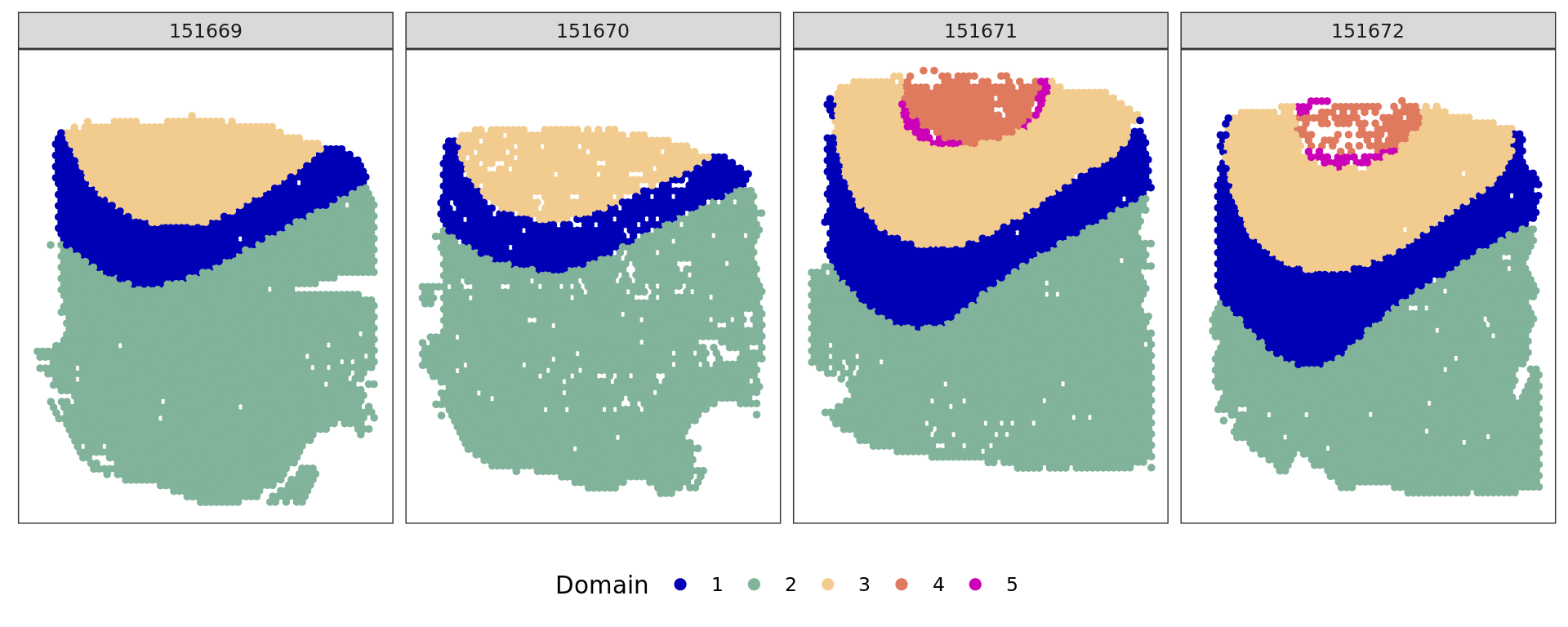
kk_UMAP_Br5595=kk_UMAP
samples_Br5595=samples
xy_Br5595=xy
labels_Br5595=labels
subject_names_Br5595=subject_names
ref_Br5595=ref
clu_Br5595=clu
save(kk_UMAP_Br5595,samples_Br5595,xy_Br5595,labels_Br5595,subject_names_Br5595,ref_Br5595,clu_Br5595,selFB,file="output/DLFPC-Br5595.RData")
save(data_Br5595,pca_Br5595,samples_Br5595,xy_Br5595,labels_Br5595,subject_names_Br5595,selFB,file="data/DLFPC-Br5595-input.RData")Patient Br5292
subject_names="Br5292"
nclusters=7
spe_sub <- spe[, colData(spe)$subject == subject_names]
dim(spe_sub)[1] 6623 17734# spe_sub <- runPCA(spe_sub, 50,subset_row = top[1:gene_number], scale=TRUE)
#pca=reducedDim(spe_sub,type = "PCA")[,1:50]
spe_sub <- spe[, colData(spe)$subject == subject_names]
sel= subjects == subject_names
data_Br5292=data[sel,top[1:gene_number]]
RNA.scaled=scale(data_Br5292)
pca_results <- irlba(A = RNA.scaled, nv = 50)
pca_Br5292 <- pca_results$u %*% diag(pca_results$d)[,1:50]
rownames(pca_Br5292)=rownames(data_Br5292)
colnames(pca_Br5292)=paste("PC",1:50,sep="")
labels=as.factor(colData(spe_sub)$layer_guess_reordered)
names(labels)=rownames(colData(spe_sub))
xy=as.matrix(spatialCoords(spe_sub))
rownames(xy)=rownames(colData(spe_sub))
samples=colData(spe_sub)$sample_id
plot(pca_Br5292, pch=20,col=as.factor(colData(spe_sub)$sample_id))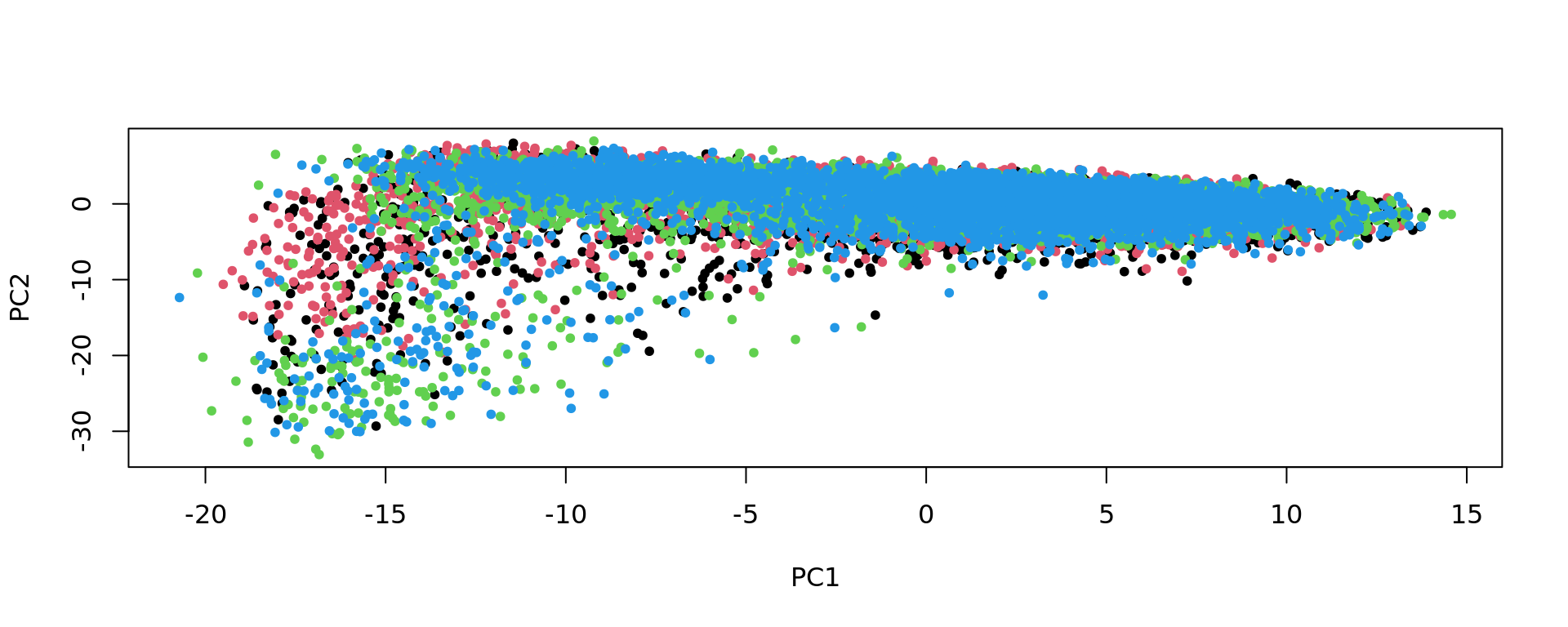
KODAMA analysis
set.seed(seed)
kk=KODAMA.matrix.parallel(pca_Br5292,
spatial = xy,
samples=samples,
FUN= "PLS" ,
landmarks = 100000,
splitting = splitting,
f.par.pls = 50,
spatial.resolution = spatial.resolution,
n.cores=n.cores,
aa_noise=aa_noise,
seed = seed)Calculating Network
Calculating Network spatial
socket cluster with 40 nodes on host 'localhost'
================================================================================
Finished parallel computation
[1] "Calculation of dissimilarity matrix..."
================================================================================ print("KODAMA finished")[1] "KODAMA finished" config=umap.defaults
config$n_threads = n.cores
config$n_sgd_threads = "auto"
kk_UMAP=KODAMA.visualization(kk,method="UMAP",config=config)
plot(kk_UMAP,pch=20,col=as.factor(labels))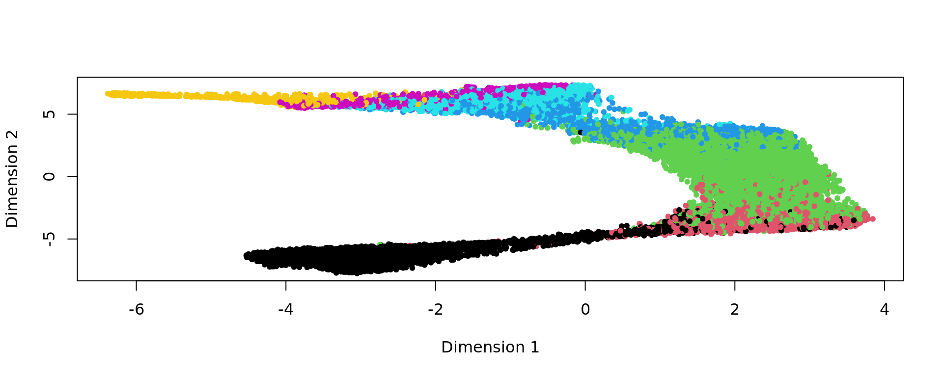
Graph-based clustering
# Graph-based clustering
g <- bluster::makeSNNGraph(as.matrix(kk_UMAP), k = graph)
g_walk <- igraph::cluster_walktrap(g)
clu <- as.character(igraph::cut_at(g_walk, no = nclusters))
plot(kk_UMAP,pch=20,col=as.factor(clu))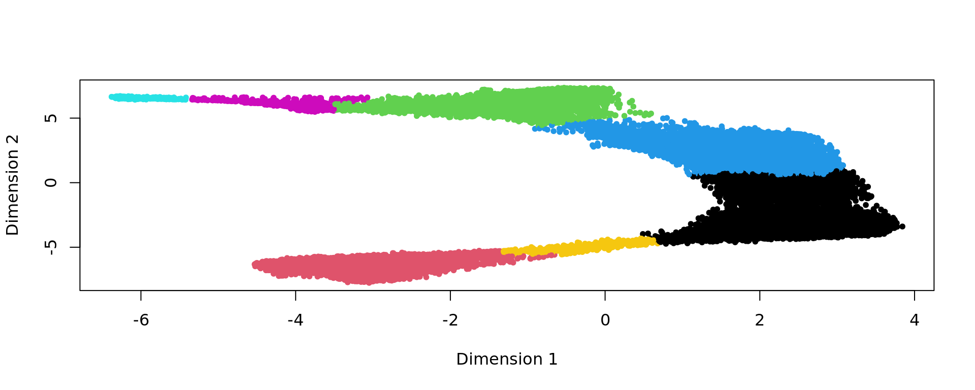
ref=refine_SVM(xy,clu,samples,cost=100)[1] "151507"
[1] "151508"
[1] "151509"
[1] "151510" u=unique(samples)
for(j in u){
sel=samples==j
print(mclust::adjustedRandIndex(labels[sel],ref[sel]))
}[1] 0.4816022
[1] 0.522308
[1] 0.4649832
[1] 0.4428301 ###########
g <- bluster::makeSNNGraph(as.matrix(kk_UMAP), k = graph)
g_walk <- igraph::cluster_walktrap(g)
clu <- as.character(igraph::cut_at(g_walk, no = nclusters))
ref=refine_SVM(xy,clu,samples,cost=100)[1] "151507"
[1] "151508"
[1] "151509"
[1] "151510" u=unique(samples)
for(j in u){
sel=samples==j
print(mclust::adjustedRandIndex(labels[sel],ref[sel]))
}[1] 0.4816022
[1] 0.522308
[1] 0.4649832
[1] 0.4428301 ###########
cols_cluster <- c("#0000b6", "#81b29a", "#f2cc8f","#e07a5f",
"#cc00b6", "#81ccff", "#33b233")
plot_slide(xy,samples,ref,col=cols_cluster)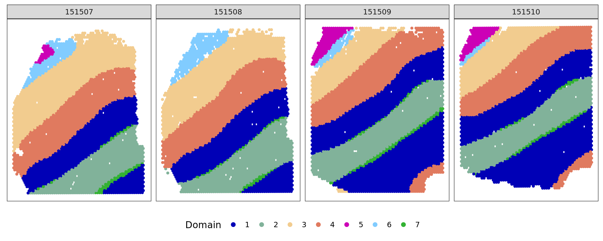
kk_UMAP_Br5292=kk_UMAP
samples_Br5292=samples
xy_Br5292=xy
labels_Br5292=labels
subject_names_Br5292=subject_names
ref_Br5292=ref
clu_Br5292=clu
save(kk_UMAP_Br5292,pca_Br5292,samples_Br5292,xy_Br5292,subject_names_Br5292,labels_Br5292,ref_Br5292,clu_Br5292,file="output/DLFPC-Br5292.RData")
save(data_Br5292,pca_Br5292,samples_Br5292,xy_Br5292,labels_Br5292,subject_names_Br5292,file="data/DLFPC-Br5292-input.RData")Patient Br8100
subject_names="Br8100"
nclusters=7
spe_sub <- spe[, colData(spe)$subject == subject_names]
dim(spe_sub)[1] 6623 13938# spe_sub <- runPCA(spe_sub, 50,subset_row = top[1:gene_number], scale=TRUE)
#pca=reducedDim(spe_sub,type = "PCA")[,1:50]
spe_sub <- spe[, colData(spe)$subject == subject_names]
sel= subjects == subject_names
data_Br8100=data[sel,top[1:gene_number]]
RNA.scaled=scale(data_Br8100)
pca_results <- irlba(A = RNA.scaled, nv = 50)
pca_Br8100 <- pca_results$u %*% diag(pca_results$d)[,1:50]
rownames(pca_Br8100)=rownames(data_Br8100)
colnames(pca_Br8100)=paste("PC",1:50,sep="")
labels=as.factor(colData(spe_sub)$layer_guess_reordered)
names(labels)=rownames(colData(spe_sub))
xy=as.matrix(spatialCoords(spe_sub))
rownames(xy)=rownames(colData(spe_sub))
samples=colData(spe_sub)$sample_id
plot(pca_Br8100, pch=20,col=as.factor(colData(spe_sub)$sample_id))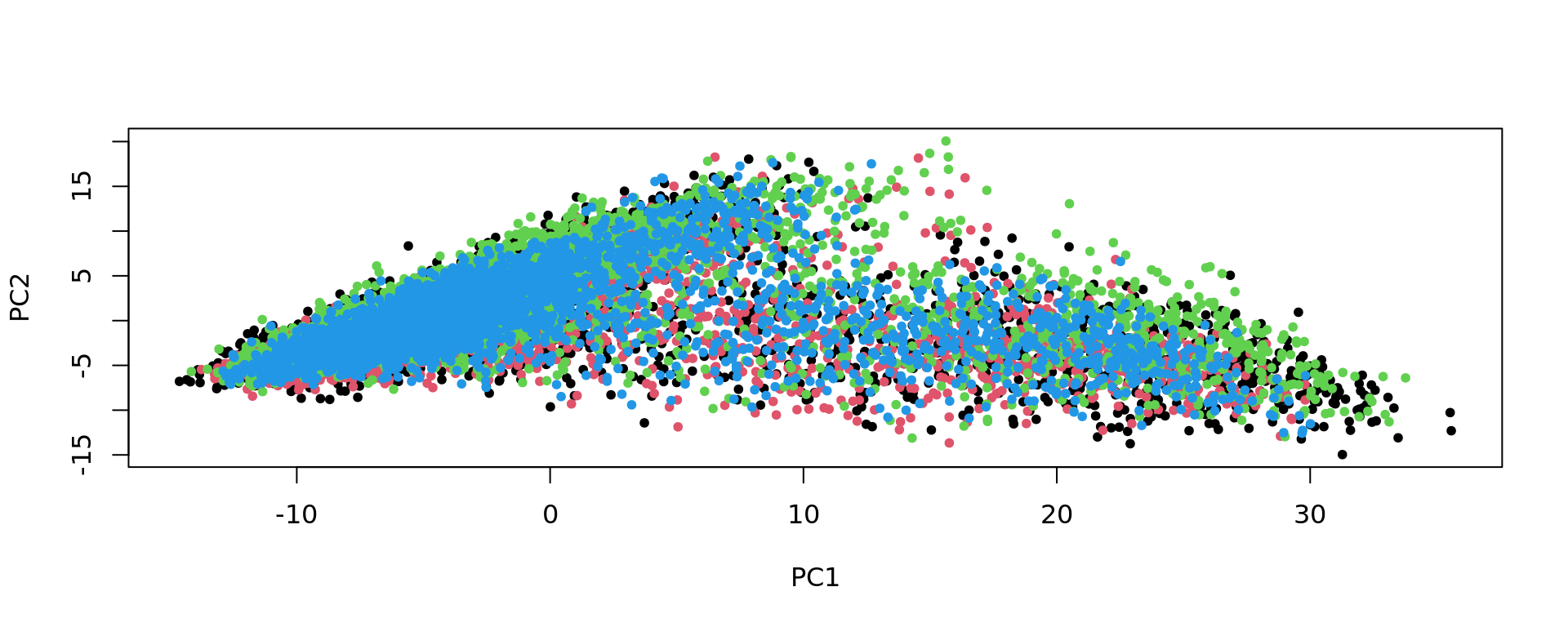
KODAMA analysis
set.seed(seed)
kk=KODAMA.matrix.parallel(pca_Br8100,
spatial = xy,
samples=samples,
FUN= "PLS" ,
landmarks = 100000,
splitting = splitting,
f.par.pls = 50,
spatial.resolution = spatial.resolution,
n.cores=n.cores,
aa_noise=aa_noise,
seed = seed)Calculating Network
Calculating Network spatial
socket cluster with 40 nodes on host 'localhost'
================================================================================
Finished parallel computation
[1] "Calculation of dissimilarity matrix..."
================================================================================ print("KODAMA finished")[1] "KODAMA finished" config=umap.defaults
config$n_threads = n.cores
config$n_sgd_threads = "auto"
kk_UMAP=KODAMA.visualization(kk,method="UMAP",config=config)
plot(kk_UMAP,pch=20,col=as.factor(labels))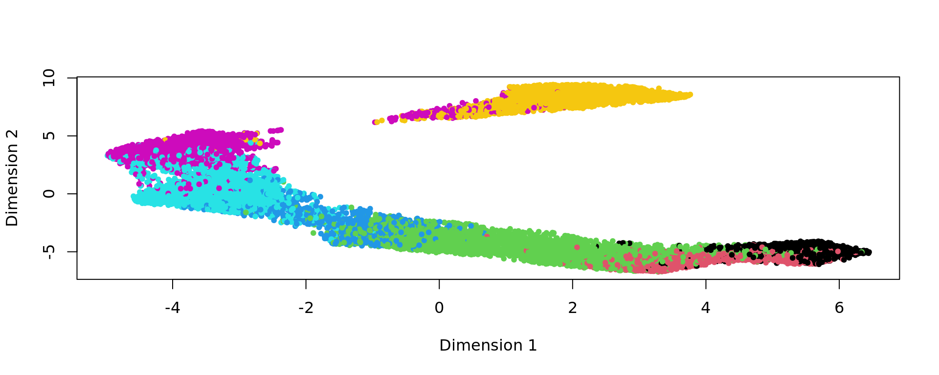
Graph-based clustering
# Graph-based clustering
g <- bluster::makeSNNGraph(as.matrix(kk_UMAP), k = graph)
g_walk <- igraph::cluster_walktrap(g)
clu <- as.character(igraph::cut_at(g_walk, no = nclusters))
ref=refine_SVM(xy,clu,samples,cost=100)[1] "151673"
[1] "151674"
[1] "151675"
[1] "151676" u=unique(samples)
for(j in u){
sel=samples==j
print(mclust::adjustedRandIndex(labels[sel],ref[sel]))
}[1] 0.5925319
[1] 0.6698008
[1] 0.6271936
[1] 0.6138289 ###########
g <- bluster::makeSNNGraph(as.matrix(kk_UMAP), k = graph)
g_walk <- igraph::cluster_walktrap(g)
clu <- as.character(igraph::cut_at(g_walk, no = nclusters))
plot(kk_UMAP,pch=20,col=as.factor(clu))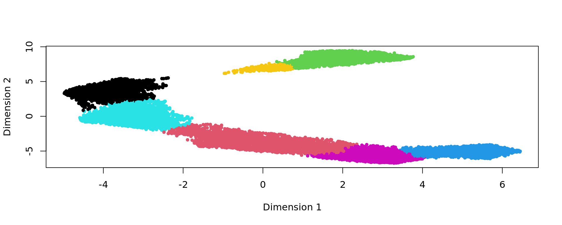
ref=refine_SVM(xy,clu,samples,cost=100)[1] "151673"
[1] "151674"
[1] "151675"
[1] "151676" u=unique(samples)
for(j in u){
sel=samples==j
print(mclust::adjustedRandIndex(labels[sel],ref[sel]))
}[1] 0.5925319
[1] 0.6698008
[1] 0.6271936
[1] 0.6138289 ###########
cols_cluster <- c("#0000b6", "#81b29a", "#f2cc8f","#e07a5f",
"#cc00b6", "#81ccff", "#33b233")
plot_slide(xy,samples,ref,col=cols_cluster)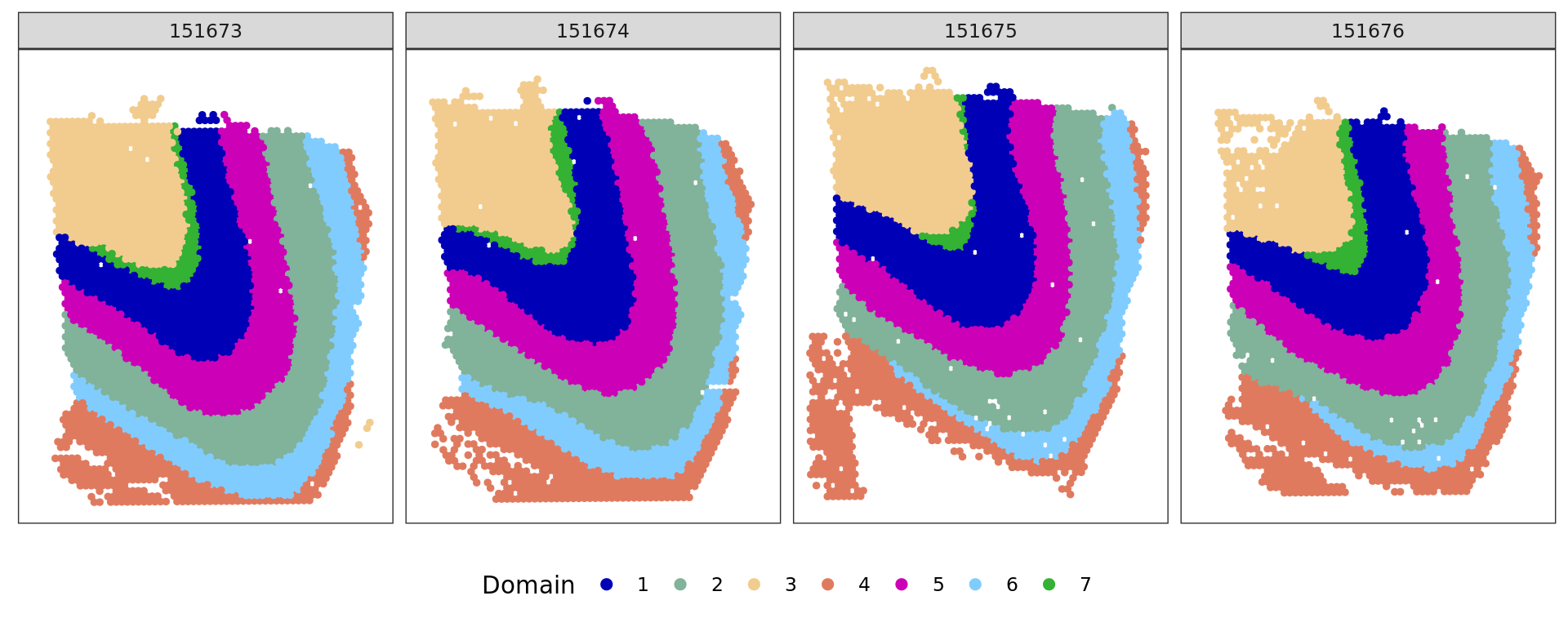
kk_UMAP_Br8100=kk_UMAP
samples_Br8100=samples
xy_Br8100=xy
labels_Br8100=labels
subject_names_Br8100=subject_names
ref_Br8100=ref
clu_Br8100=clu
save(kk_UMAP_Br8100,pca_Br8100,samples_Br8100,xy_Br8100,subject_names_Br8100,labels_Br8100,ref_Br8100,clu_Br8100,file="output/DLFPC-Br8100.RData")
save(data_Br8100,pca_Br8100,samples_Br8100,xy_Br8100,labels_Br8100,subject_names_Br8100,file="data/DLFPC-Br8100-input.RData")Saving the results
results_KODAMA <- list()
results_KODAMA$cluster <- list()
results_KODAMA$feature_extraction <- list()
results_KODAMA$cluster=c(results_KODAMA$cluster,tapply(ref_Br5292,samples_Br5292,function(x) x))
results_KODAMA$cluster=c(results_KODAMA$cluster,tapply(ref_Br5595,samples_Br5595,function(x) x))
results_KODAMA$cluster=c(results_KODAMA$cluster,tapply(ref_Br8100,samples_Br8100,function(x) x))
results_KODAMA$feature_extraction=c(results_KODAMA$feature_extraction,by(kk_UMAP_Br5292,samples_Br5292,function(x) x))
results_KODAMA$feature_extraction=c(results_KODAMA$feature_extraction,by(kk_UMAP_Br5595,samples_Br5595,function(x) x))
results_KODAMA$feature_extraction=c(results_KODAMA$feature_extraction,by(kk_UMAP_Br8100,samples_Br8100,function(x) x))
save(results_KODAMA,file="output/KODAMA-results.RData")#seurat list preprocessing
source("code/DLFPC_preprocessing.R")[1] 1
[1] 2
[1] 3
[1] 4
[1] 5
[1] 6
[1] 7
[1] 8
[1] 9
[1] 10
[1] 11
[1] 1212 Slides
PCA and HARMONY
dim(spe_sub)[1] 6623 13938 spe <- runPCA(spe, 50,subset_row = top[1:gene_number], scale=TRUE)
subjects=colData(spe)$subject
labels=as.factor(colData(spe)$layer_guess_reordered)
xy=as.matrix(spatialCoords(spe))
samples=colData(spe)$sample_id
spe <- RunHarmony(spe, "subject",lambda=NULL)
pca=reducedDim(spe,type = "HARMONY")[,1:50]
plot(pca, pch=20,col=as.factor(colData(spe_sub)$sample_id))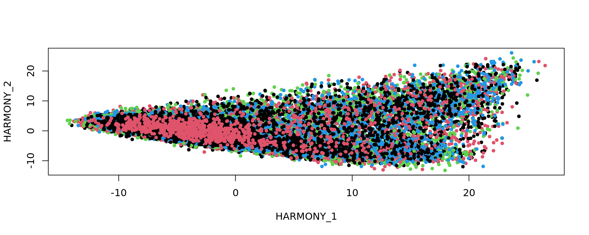
KODAMA
set.seed(seed)
kk=KODAMA.matrix.parallel(pca,
spatial = xy,
samples=samples,
FUN= "PLS" ,
landmarks = 100000,
splitting = 300,
f.par.pls = 50,
spatial.resolution = spatial.resolution,
n.cores=n.cores,
aa_noise=aa_noise,
seed = seed)Calculating Network
Calculating Network spatial
socket cluster with 40 nodes on host 'localhost'
================================================================================
Finished parallel computation
[1] "Calculation of dissimilarity matrix..."
================================================================================print("KODAMA finished")[1] "KODAMA finished"config=umap.defaults
config$n_threads = n.cores
config$n_sgd_threads = "auto"
kk_UMAP=KODAMA.visualization(kk,method="UMAP",config=config)
plot(kk_UMAP,pch=20,col=as.factor(labels))
CLUSTER
g <- bluster::makeSNNGraph(as.matrix(kk_UMAP), k = graph)
g_walk <- igraph::cluster_walktrap(g)
clu <- as.character(igraph::cut_at(g_walk, no = 7))
plot(kk_UMAP,pch=20,col=as.factor(clu)) 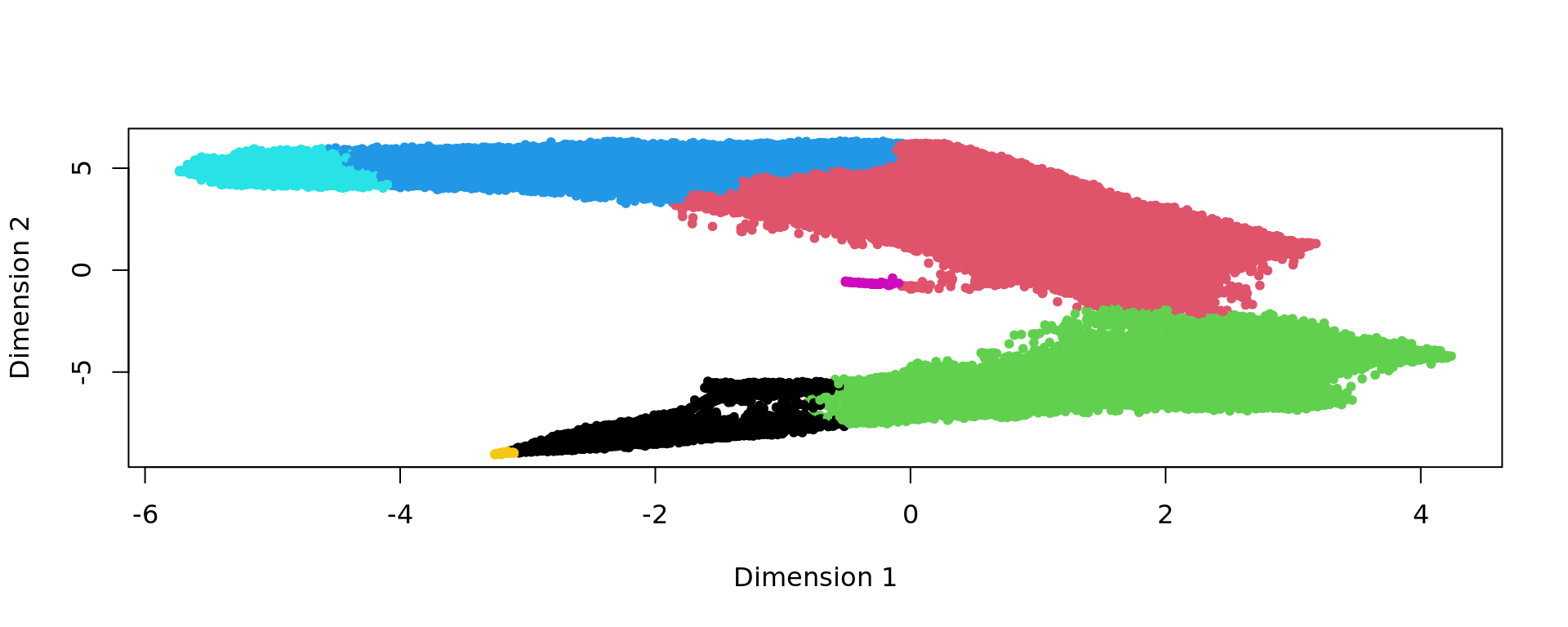
ref=refine_SVM(xy,clu,samples,cost=100)[1] "151507"
[1] "151508"
[1] "151509"
[1] "151510"
[1] "151669"
[1] "151670"
[1] "151671"
[1] "151672"
[1] "151673"
[1] "151674"
[1] "151675"
[1] "151676"cols_cluster <- c("#0000b6", "#81b29a", "#f2cc8f","#e07a5f",
"#cc00b6", "#81ccff", "#33b233")
plot_slide(xy,samples,ref,col=cols_cluster)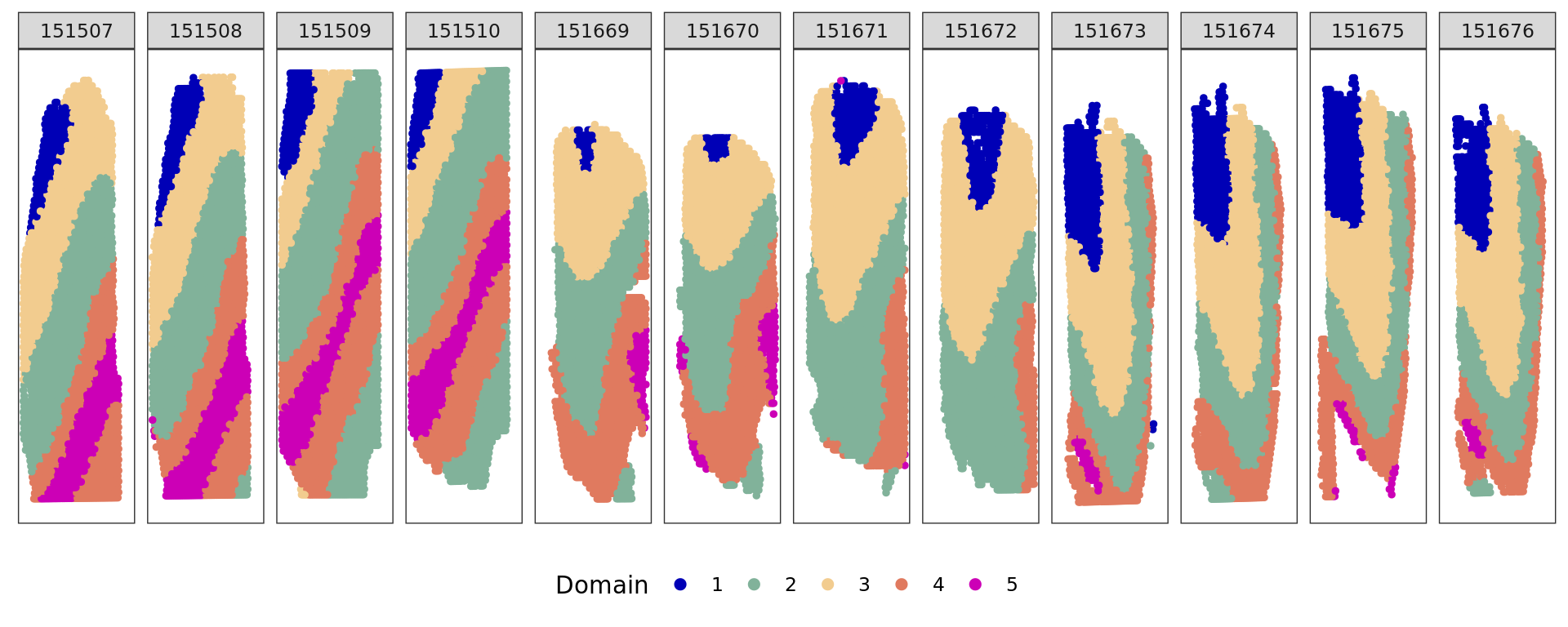
CLUSTER
clu=kmeans(kk_UMAP,7,nstart = 100)$cluster
plot(kk_UMAP,col=labels,pch=20)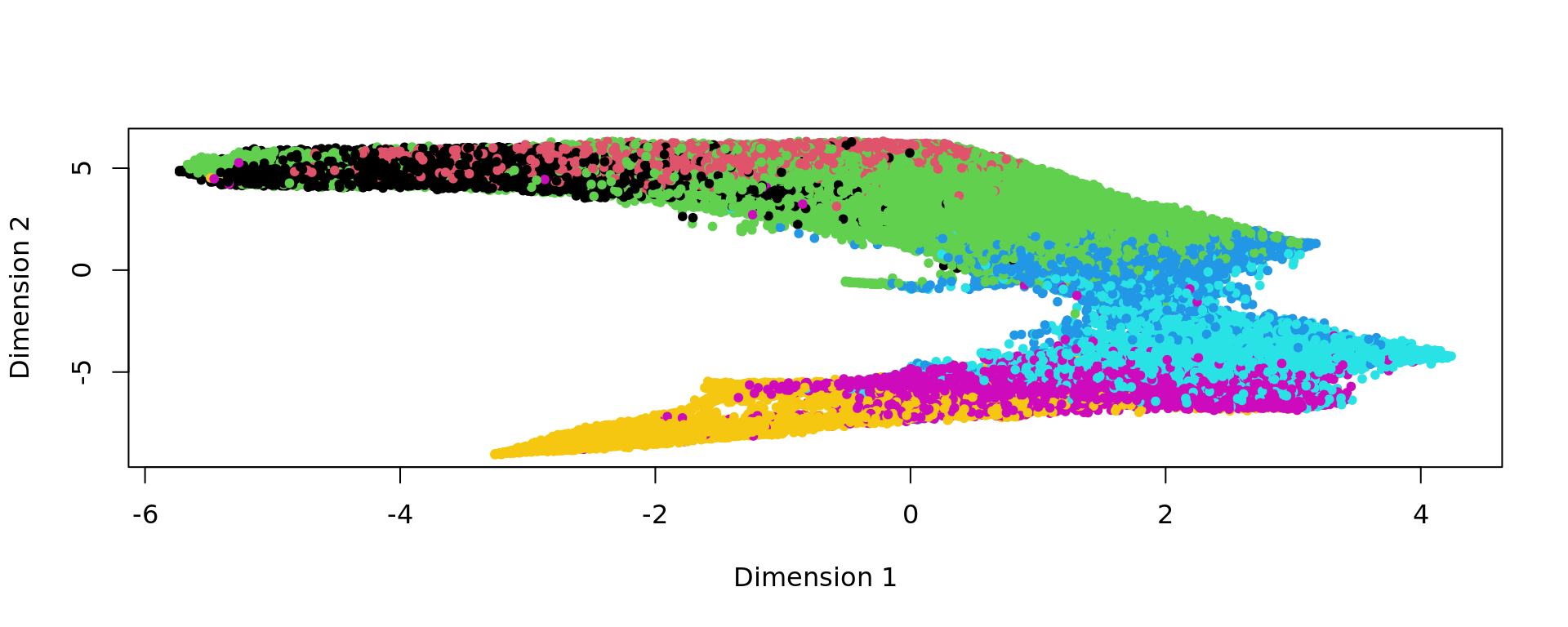
plot(kk_UMAP,col=cols_cluster[clu],pch=20)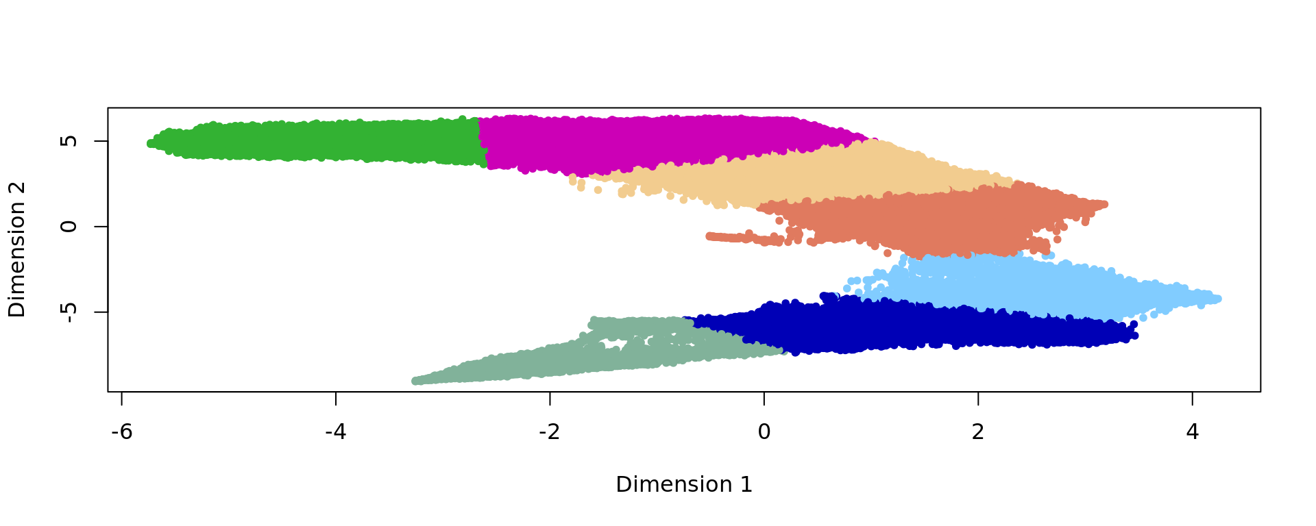
u=unique(samples)
for(i in 1:length(u)){
sel=samples==u[i]
print(adjustedRandIndex(labels[sel],clu[sel]))
}[1] 0.5284518
[1] 0.4909196
[1] 0.4830495
[1] 0.4689889
[1] 0.3425394
[1] 0.3187019
[1] 0.3771417
[1] 0.416698
[1] 0.5466472
[1] 0.555753
[1] 0.5436048
[1] 0.5270994ref=refine_SVM(xy,clu,samples,cost=100)[1] "151507"
[1] "151508"
[1] "151509"
[1] "151510"
[1] "151669"
[1] "151670"
[1] "151671"
[1] "151672"
[1] "151673"
[1] "151674"
[1] "151675"
[1] "151676"
u=unique(samples)
for(i in 1:length(u)){
sel=samples==u[i]
print(adjustedRandIndex(labels[sel],ref[sel]))
}[1] 0.5737931
[1] 0.5208063
[1] 0.4923182
[1] 0.4875874
[1] 0.385967
[1] 0.3768955
[1] 0.448543
[1] 0.5415363
[1] 0.5919723
[1] 0.5990537
[1] 0.609972
[1] 0.5886862plot_slide(xy,samples,ref,col=cols_cluster)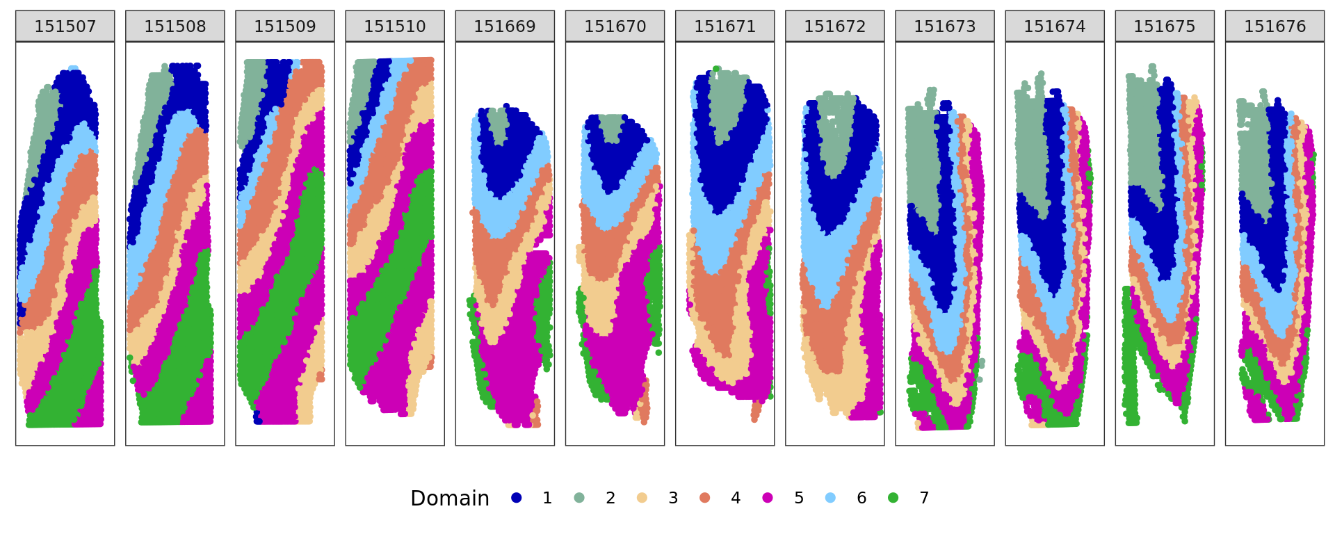
| Version | Author | Date |
|---|---|---|
| fd8d092 | Stefano Cacciatore | 2024-10-15 |
TRAJECTORY
d <- slingshot(kk_UMAP, clusterLabels = clu)
trajectory=d@metadata$curves$Lineage1$s
k=knn_Armadillo(trajectory,kk_UMAP,1)
map_color=rainbow(nrow(trajectory))[k$nn_index]
plot(kk_UMAP,pch=20,col=map_color)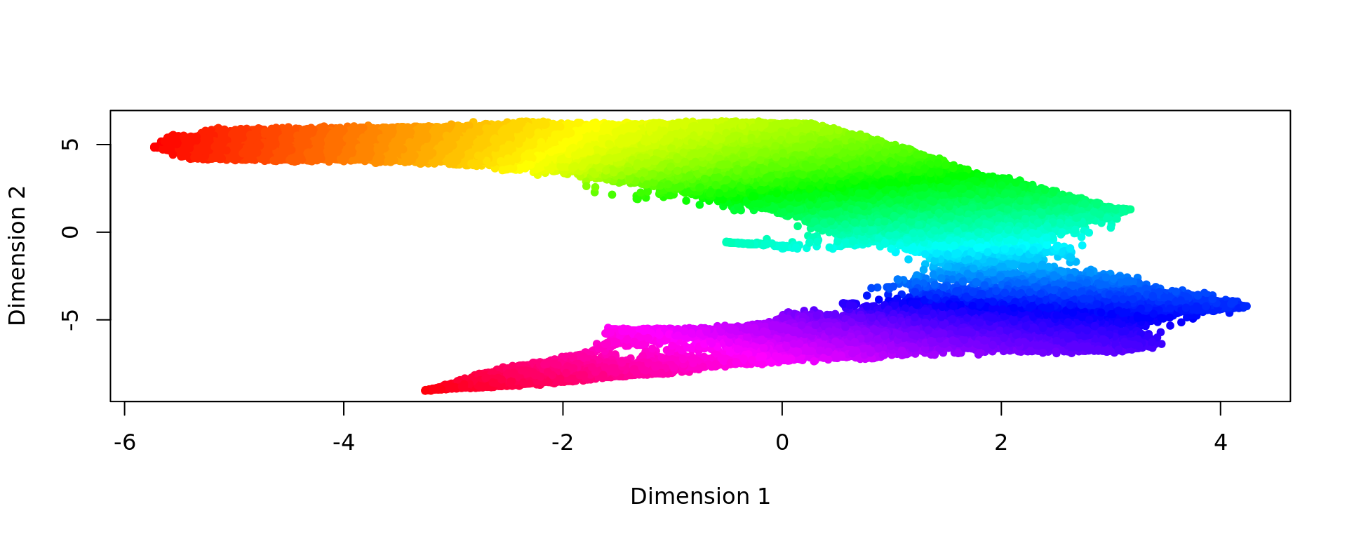
plot_slide(xy,samples,k$nn_index,col=rainbow(nrow(trajectory)))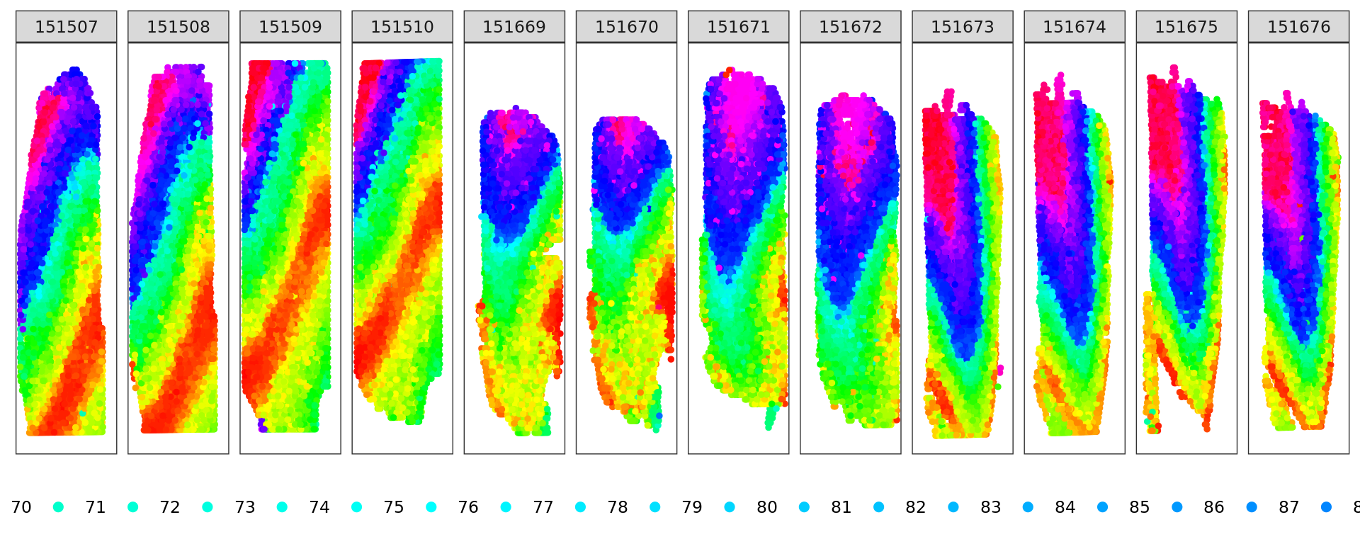
| Version | Author | Date |
|---|---|---|
| fd8d092 | Stefano Cacciatore | 2024-10-15 |
source("code/DLPFC_comparison.R")[1] 7
[1] 1
[1] 2
[1] 2
[1] 2
[1] 2
[1] 2
[1] 2
[1] 3
[1] 4
[1] 4
[1] 4
[1] 4
[1] 4
[1] 5
[1] 5
[1] 5
[1] 5
[1] 5
[1] 5
[1] 5
[1] 6
[1] 6
[1] 6
[1] 7
[1] 4
[1] 4
[1] 4
[1] 4
[1] 4
[1] 4
[1] 4
[1] 5
[1] 1
[1] 1
[1] 1
[1] 2
[1] 2
[1] 3
[1] 3
[1] 3
[1] 3
[1] 3
[1] 4
[1] 4
[1] 4
[1] 4
[1] 4
[1] 5
[1] 7
[1] 2
[1] 2
[1] 2
[1] 2
[1] 2
[1] 2
[1] 3
[1] 3
[1] 4
[1] 4
[1] 4
[1] 4
[1] 4
[1] 4
[1] 4
[1] 4
[1] 4
[1] 6
[1] 5
[1] 6
[1] 7
***************************************
INPUT INFO:
- Number of tissue sections: 4
- Number of cells/spots: 4170 4285 4708 4571
- Number of genes: 2000
- Potts interaction parameter estimation method: SW
- Estimate Potts interaction parameter with SW algorithm
To list all hyper-parameters, Type listAllHyper(BASS_object)
***************************************
Post-processing...
done
***************************************
INPUT INFO:
- Number of tissue sections: 4
- Number of cells/spots: 3587 3274 4013 3772
- Number of genes: 2000
- Potts interaction parameter estimation method: SW
- Estimate Potts interaction parameter with SW algorithm
To list all hyper-parameters, Type listAllHyper(BASS_object)
***************************************
Post-processing...
done
***************************************
INPUT INFO:
- Number of tissue sections: 4
- Number of cells/spots: 3568 3576 3468 3326
- Number of genes: 2000
- Potts interaction parameter estimation method: SW
- Estimate Potts interaction parameter with SW algorithm
To list all hyper-parameters, Type listAllHyper(BASS_object)
***************************************
Post-processing...
done
fitting ...
| | | 0% | |=================================== | 50% | |======================================================================| 100%
variable initialize finish!
predict Y and V!
diff Energy = 1.953018
diff Energy = 8.141713
diff Energy = 19.443110
diff Energy = 2.580638
Finish ICM step!
iter = 2, loglik= -13930299.000000, dloglik=0.993513
predict Y and V!
diff Energy = 3.343862
diff Energy = 1.076378
diff Energy = 16.470758
diff Energy = 3.114019
Finish ICM step!
iter = 3, loglik= -13855945.000000, dloglik=0.005338
predict Y and V!
diff Energy = 10.926458
diff Energy = 12.746197
diff Energy = 17.945403
diff Energy = 10.686093
Finish ICM step!
iter = 4, loglik= -13826536.000000, dloglik=0.002122
predict Y and V!
diff Energy = 12.373065
diff Energy = 7.074120
diff Energy = 24.492056
diff Energy = 19.422095
Finish ICM step!
iter = 5, loglik= -13812401.000000, dloglik=0.001022
predict Y and V!
diff Energy = 12.534292
diff Energy = 7.827485
diff Energy = 31.227270
diff Energy = 12.679315
Finish ICM step!
iter = 6, loglik= -13804297.000000, dloglik=0.000587
predict Y and V!
diff Energy = 7.976928
diff Energy = 12.374174
diff Energy = 35.633381
diff Energy = 14.944129
Finish ICM step!
iter = 7, loglik= -13799340.000000, dloglik=0.000359
predict Y and V!
diff Energy = 7.718569
diff Energy = 8.578184
diff Energy = 22.873074
diff Energy = 12.299571
Finish ICM step!
iter = 8, loglik= -13796130.000000, dloglik=0.000233
predict Y and V!
diff Energy = 6.616963
diff Energy = 4.701413
diff Energy = 19.178816
diff Energy = 10.107264
Finish ICM step!
iter = 9, loglik= -13793975.000000, dloglik=0.000156
predict Y and V!
diff Energy = 5.563113
diff Energy = 11.360947
diff Energy = 20.831881
diff Energy = 6.159683
Finish ICM step!
iter = 10, loglik= -13792445.000000, dloglik=0.000111
predict Y and V!
diff Energy = 1.923684
diff Energy = 10.232090
diff Energy = 20.112130
diff Energy = 4.056136
Finish ICM step!
iter = 11, loglik= -13791317.000000, dloglik=0.000082
predict Y and V!
diff Energy = 3.979426
diff Energy = 8.213570
diff Energy = 23.118767
diff Energy = 11.890381
Finish ICM step!
iter = 12, loglik= -13790474.000000, dloglik=0.000061
predict Y and V!
diff Energy = 0.517123
diff Energy = 5.708328
diff Energy = 26.217663
diff Energy = 12.489663
Finish ICM step!
iter = 13, loglik= -13789809.000000, dloglik=0.000048
predict Y and V!
diff Energy = 4.868877
diff Energy = 11.706409
diff Energy = 19.387300
diff Energy = 9.421632
Finish ICM step!
iter = 14, loglik= -13789288.000000, dloglik=0.000038
predict Y and V!
diff Energy = 0.167818
diff Energy = 6.425094
diff Energy = 25.762972
diff Energy = 4.255616
Finish ICM step!
iter = 15, loglik= -13788862.000000, dloglik=0.000031
predict Y and V!
diff Energy = 6.157080
diff Energy = 9.561001
diff Energy = 20.982824
diff Energy = 9.972268
Finish ICM step!
iter = 16, loglik= -13788518.000000, dloglik=0.000025
predict Y and V!
diff Energy = 0.811254
diff Energy = 9.090096
diff Energy = 22.996069
diff Energy = 12.289073
Finish ICM step!
iter = 17, loglik= -13788236.000000, dloglik=0.000020
predict Y and V!
diff Energy = 5.597086
diff Energy = 7.522623
diff Energy = 23.225553
diff Energy = 21.973080
Finish ICM step!
iter = 18, loglik= -13788006.000000, dloglik=0.000017
predict Y and V!
diff Energy = 6.266428
diff Energy = 2.871766
diff Energy = 23.844093
diff Energy = 14.426780
Finish ICM step!
iter = 19, loglik= -13787809.000000, dloglik=0.000014
predict Y and V!
diff Energy = 5.076429
diff Energy = 8.608232
diff Energy = 26.371702
diff Energy = 15.465027
Finish ICM step!
iter = 20, loglik= -13787643.000000, dloglik=0.000012
predict Y and V!
diff Energy = 2.606656
diff Energy = 2.685831
diff Energy = 29.903853
diff Energy = 17.212277
Finish ICM step!
iter = 21, loglik= -13787490.000000, dloglik=0.000011
predict Y and V!
diff Energy = 5.676004
diff Energy = 3.783376
diff Energy = 29.372576
diff Energy = 11.489312
Finish ICM step!
iter = 22, loglik= -13787365.000000, dloglik=0.000009
fitting ...
| | | 0% | |=================================== | 50% | |======================================================================| 100%
variable initialize finish!
predict Y and V!
diff Energy = 2.565470
diff Energy = 0.584042
diff Energy = 6.057265
diff Energy = 3.061791
Finish ICM step!
iter = 2, loglik= -9972800.000000, dloglik=0.995356
predict Y and V!
diff Energy = 14.114203
diff Energy = 1.165911
diff Energy = 0.753432
diff Energy = 1.194389
Finish ICM step!
iter = 3, loglik= -9914716.000000, dloglik=0.005824
predict Y and V!
diff Energy = 20.161622
diff Energy = 3.189229
diff Energy = 19.531276
diff Energy = 10.980305
Finish ICM step!
iter = 4, loglik= -9891159.000000, dloglik=0.002376
predict Y and V!
diff Energy = 19.147380
diff Energy = 10.431936
diff Energy = 2.947157
diff Energy = 6.377402
Finish ICM step!
iter = 5, loglik= -9879672.000000, dloglik=0.001161
predict Y and V!
diff Energy = 22.060679
diff Energy = 8.820266
diff Energy = 17.204482
diff Energy = 9.850850
Finish ICM step!
iter = 6, loglik= -9873269.000000, dloglik=0.000648
predict Y and V!
diff Energy = 17.484536
diff Energy = 13.904037
diff Energy = 0.970989
diff Energy = 7.993890
Finish ICM step!
iter = 7, loglik= -9869452.000000, dloglik=0.000387
predict Y and V!
diff Energy = 18.583919
diff Energy = 13.488603
diff Energy = 13.056635
diff Energy = 5.918180
Finish ICM step!
iter = 8, loglik= -9867032.000000, dloglik=0.000245
predict Y and V!
diff Energy = 13.752026
diff Energy = 22.456746
diff Energy = 0.517486
diff Energy = 8.704953
Finish ICM step!
iter = 9, loglik= -9865406.000000, dloglik=0.000165
predict Y and V!
diff Energy = 14.655218
diff Energy = 13.808834
diff Energy = 1.747965
diff Energy = 8.778440
Finish ICM step!
iter = 10, loglik= -9864276.000000, dloglik=0.000115
predict Y and V!
diff Energy = 13.660964
diff Energy = 17.445726
diff Energy = 2.945565
diff Energy = 5.123273
Finish ICM step!
iter = 11, loglik= -9863453.000000, dloglik=0.000083
predict Y and V!
diff Energy = 13.294779
diff Energy = 17.479028
diff Energy = 4.355807
diff Energy = 11.960606
Finish ICM step!
iter = 12, loglik= -9862866.000000, dloglik=0.000060
predict Y and V!
diff Energy = 13.146640
diff Energy = 20.702204
diff Energy = 1.542905
diff Energy = 7.328645
Finish ICM step!
iter = 13, loglik= -9862424.000000, dloglik=0.000045
predict Y and V!
diff Energy = 11.795079
diff Energy = 14.734103
diff Energy = 6.337264
diff Energy = 9.458880
Finish ICM step!
iter = 14, loglik= -9862076.000000, dloglik=0.000035
predict Y and V!
diff Energy = 12.161588
diff Energy = 13.036398
diff Energy = 6.881132
diff Energy = 10.586986
Finish ICM step!
iter = 15, loglik= -9861799.000000, dloglik=0.000028
predict Y and V!
diff Energy = 12.208746
diff Energy = 11.393562
diff Energy = 5.504740
diff Energy = 11.358293
Finish ICM step!
iter = 16, loglik= -9861573.000000, dloglik=0.000023
predict Y and V!
diff Energy = 15.334242
diff Energy = 6.691065
diff Energy = 3.301489
diff Energy = 15.225853
Finish ICM step!
iter = 17, loglik= -9861396.000000, dloglik=0.000018
predict Y and V!
diff Energy = 4.765992
diff Energy = 9.942739
diff Energy = 6.590917
diff Energy = 0.381692
Finish ICM step!
iter = 18, loglik= -9861231.000000, dloglik=0.000017
predict Y and V!
diff Energy = 3.507494
diff Energy = 6.647690
diff Energy = 3.728636
diff Energy = 6.103977
Finish ICM step!
iter = 19, loglik= -9861099.000000, dloglik=0.000013
predict Y and V!
diff Energy = 4.640637
diff Energy = 9.132833
diff Energy = 1.068987
diff Energy = 3.515024
Finish ICM step!
iter = 20, loglik= -9860988.000000, dloglik=0.000011
predict Y and V!
diff Energy = 6.008195
diff Energy = 6.416183
diff Energy = 4.608951
diff Energy = 3.900260
Finish ICM step!
iter = 21, loglik= -9860887.000000, dloglik=0.000010
predict Y and V!
diff Energy = 5.022243
diff Energy = 7.741218
diff Energy = 0.879150
diff Energy = 6.282546
Finish ICM step!
iter = 22, loglik= -9860798.000000, dloglik=0.000009
fitting ...
| | | 0% | |=================================== | 50% | |======================================================================| 100%
variable initialize finish!
predict Y and V!
diff Energy = 6.154259
diff Energy = 0.674600
diff Energy = 21.472756
diff Energy = 3.920762
Finish ICM step!
iter = 2, loglik= -9267840.000000, dloglik=0.995684
predict Y and V!
diff Energy = 9.144959
diff Energy = 0.370867
diff Energy = 14.004674
diff Energy = 4.651187
Finish ICM step!
iter = 3, loglik= -9207665.000000, dloglik=0.006493
predict Y and V!
diff Energy = 18.268786
diff Energy = 12.287058
diff Energy = 31.479777
diff Energy = 31.660518
Finish ICM step!
iter = 4, loglik= -9182367.000000, dloglik=0.002747
predict Y and V!
diff Energy = 32.759643
diff Energy = 18.929512
diff Energy = 29.591938
diff Energy = 11.306277
Finish ICM step!
iter = 5, loglik= -9169607.000000, dloglik=0.001390
predict Y and V!
diff Energy = 24.618622
diff Energy = 21.819884
diff Energy = 34.194294
diff Energy = 14.214422
Finish ICM step!
iter = 6, loglik= -9162353.000000, dloglik=0.000791
predict Y and V!
diff Energy = 24.780251
diff Energy = 6.760886
diff Energy = 24.640985
diff Energy = 14.435737
Finish ICM step!
iter = 7, loglik= -9157901.000000, dloglik=0.000486
predict Y and V!
diff Energy = 30.391947
diff Energy = 11.457682
diff Energy = 28.493764
diff Energy = 21.204576
Finish ICM step!
iter = 8, loglik= -9155034.000000, dloglik=0.000313
predict Y and V!
diff Energy = 22.595902
diff Energy = 7.759056
diff Energy = 6.491424
diff Energy = 18.470470
Finish ICM step!
iter = 9, loglik= -9153073.000000, dloglik=0.000214
predict Y and V!
diff Energy = 11.787161
diff Energy = 11.660366
diff Energy = 10.471258
diff Energy = 22.365486
Finish ICM step!
iter = 10, loglik= -9151693.000000, dloglik=0.000151
predict Y and V!
diff Energy = 20.443170
diff Energy = 4.844400
diff Energy = 6.870913
diff Energy = 22.530623
Finish ICM step!
iter = 11, loglik= -9150682.000000, dloglik=0.000110
predict Y and V!
diff Energy = 9.287491
diff Energy = 2.055274
diff Energy = 10.272830
diff Energy = 25.210668
Finish ICM step!
iter = 12, loglik= -9149904.000000, dloglik=0.000085
predict Y and V!
diff Energy = 9.850887
diff Energy = 3.479769
diff Energy = 2.225239
diff Energy = 25.191220
Finish ICM step!
iter = 13, loglik= -9149279.000000, dloglik=0.000068
predict Y and V!
diff Energy = 8.240278
diff Energy = 8.621623
diff Energy = 3.149501
diff Energy = 27.705288
Finish ICM step!
iter = 14, loglik= -9148850.000000, dloglik=0.000047
predict Y and V!
diff Energy = 9.282241
diff Energy = 0.394975
diff Energy = 1.471517
diff Energy = 28.640782
Finish ICM step!
iter = 15, loglik= -9148410.000000, dloglik=0.000048
predict Y and V!
diff Energy = 9.232025
diff Energy = 3.868532
diff Energy = 5.221636
diff Energy = 24.500799
Finish ICM step!
iter = 16, loglik= -9148068.000000, dloglik=0.000037
predict Y and V!
diff Energy = 14.312273
diff Energy = 1.721576
diff Energy = 1.868712
diff Energy = 28.580078
Finish ICM step!
iter = 17, loglik= -9147758.000000, dloglik=0.000034
predict Y and V!
diff Energy = 10.519846
diff Energy = 3.306228
diff Energy = 3.078168
diff Energy = 31.128279
Finish ICM step!
iter = 18, loglik= -9147539.000000, dloglik=0.000024
predict Y and V!
diff Energy = 8.912950
diff Energy = 0.887420
diff Energy = 10.734067
diff Energy = 29.072680
Finish ICM step!
iter = 19, loglik= -9147289.000000, dloglik=0.000027
predict Y and V!
diff Energy = 9.127815
diff Energy = 3.416733
diff Energy = 0.088839
diff Energy = 31.428592
Finish ICM step!
iter = 20, loglik= -9147068.000000, dloglik=0.000024
predict Y and V!
diff Energy = 9.630816
diff Energy = 1.456853
diff Energy = 6.223830
diff Energy = 18.127232
Finish ICM step!
iter = 21, loglik= -9146873.000000, dloglik=0.000021
predict Y and V!
diff Energy = 4.558375
diff Energy = 3.492783
diff Energy = 2.248278
diff Energy = 28.422799
Finish ICM step!
iter = 22, loglik= -9146675.000000, dloglik=0.000022
predict Y and V!
diff Energy = 4.865577
diff Energy = 0.205503
diff Energy = 2.129716
diff Energy = 29.027058
Finish ICM step!
iter = 23, loglik= -9146493.000000, dloglik=0.000020
predict Y and V!
diff Energy = 6.491902
diff Energy = 2.425016
diff Energy = 31.081611
Finish ICM step!
iter = 24, loglik= -9146345.000000, dloglik=0.000016
predict Y and V!
diff Energy = 4.151331
diff Energy = 0.154580
diff Energy = 29.134086
Finish ICM step!
iter = 25, loglik= -9146171.000000, dloglik=0.000019
predict Y and V!
diff Energy = 4.601915
diff Energy = 0.466578
diff Energy = 2.671628
diff Energy = 31.407540
Finish ICM step!
iter = 26, loglik= -9146005.000000, dloglik=0.000018
predict Y and V!
diff Energy = 0.118307
diff Energy = 0.260166
diff Energy = 1.985538
diff Energy = 30.698976
Finish ICM step!
iter = 27, loglik= -9145814.000000, dloglik=0.000021
predict Y and V!
diff Energy = 3.441213
diff Energy = 1.463324
diff Energy = 8.717503
diff Energy = 25.982390
Finish ICM step!
iter = 28, loglik= -9145663.000000, dloglik=0.000017
predict Y and V!
diff Energy = 0.320328
diff Energy = 0.189082
diff Energy = 2.124648
diff Energy = 23.658331
Finish ICM step!
iter = 29, loglik= -9145508.000000, dloglik=0.000017
predict Y and V!
diff Energy = 8.075440
diff Energy = 0.761397
diff Energy = 1.202379
diff Energy = 27.614691
Finish ICM step!
iter = 30, loglik= -9145407.000000, dloglik=0.000011
sessionInfo()R version 4.4.1 (2024-06-14)
Platform: x86_64-pc-linux-gnu
Running under: Ubuntu 20.04.6 LTS
Matrix products: default
BLAS: /usr/lib/x86_64-linux-gnu/blas/libblas.so.3.9.0
LAPACK: /usr/lib/x86_64-linux-gnu/lapack/liblapack.so.3.9.0
locale:
[1] LC_CTYPE=en_US.UTF-8 LC_NUMERIC=C
[3] LC_TIME=en_US.UTF-8 LC_COLLATE=en_US.UTF-8
[5] LC_MONETARY=en_US.UTF-8 LC_MESSAGES=en_US.UTF-8
[7] LC_PAPER=en_US.UTF-8 LC_NAME=C
[9] LC_ADDRESS=C LC_TELEPHONE=C
[11] LC_MEASUREMENT=en_US.UTF-8 LC_IDENTIFICATION=C
time zone: Etc/UTC
tzcode source: system (glibc)
attached base packages:
[1] parallel stats4 stats graphics grDevices utils datasets
[8] methods base
other attached packages:
[1] BayesSpace_1.14.0 PRECAST_1.6.5
[3] gtools_3.9.5 Banksy_1.0.0
[5] BASS_1.1.0.017 GIGrvg_0.8
[7] bluster_1.14.0 igraph_2.0.3
[9] irlba_2.3.5.1 Matrix_1.7-0
[11] slingshot_2.12.0 TrajectoryUtils_1.12.0
[13] princurve_2.1.6 mclust_6.1.1
[15] KODAMAextra_1.0 bigmemory_4.6.4
[17] rgl_1.3.1 misc3d_0.9-1
[19] e1071_1.7-16 doParallel_1.0.17
[21] iterators_1.0.14 foreach_1.5.2
[23] KODAMA_3.1 umap_0.2.10.0
[25] Rtsne_0.17 minerva_1.5.10
[27] spatialLIBD_1.16.2 SpatialExperiment_1.14.0
[29] Seurat_5.1.0 SeuratObject_5.0.2
[31] sp_2.1-4 harmony_1.2.1
[33] Rcpp_1.0.13 SPARK_1.1.1
[35] scry_1.16.0 scran_1.32.0
[37] scater_1.32.1 ggplot2_3.5.1
[39] scuttle_1.14.0 SingleCellExperiment_1.26.0
[41] SummarizedExperiment_1.34.0 Biobase_2.64.0
[43] GenomicRanges_1.56.1 GenomeInfoDb_1.40.1
[45] IRanges_2.38.1 S4Vectors_0.42.1
[47] BiocGenerics_0.50.0 MatrixGenerics_1.16.0
[49] matrixStats_1.4.1 nnSVG_1.8.0
[51] workflowr_1.7.1
loaded via a namespace (and not attached):
[1] ica_1.0-3 plotly_4.10.4
[3] Formula_1.2-5 rematch2_2.1.2
[5] maps_3.4.2 zlibbioc_1.50.0
[7] tidyselect_1.2.1 bit_4.5.0
[9] lattice_0.22-6 rjson_0.2.23
[11] label.switching_1.8 blob_1.2.4
[13] stringr_1.5.1 BRISC_1.0.6
[15] S4Arrays_1.4.1 png_0.1-8
[17] cli_3.6.3 askpass_1.2.0
[19] openssl_2.2.0 goftest_1.2-3
[21] BiocIO_1.14.0 doSNOW_1.0.20
[23] purrr_1.0.2 BiocNeighbors_1.22.0
[25] uwot_0.2.2 curl_5.2.1
[27] mime_0.12 evaluate_0.24.0
[29] leiden_0.4.3.1 stringi_1.8.4
[31] backports_1.5.0 XML_3.99-0.17
[33] httpuv_1.6.15 AnnotationDbi_1.66.0
[35] paletteer_1.6.0 magrittr_2.0.3
[37] rappdirs_0.3.3 splines_4.4.1
[39] dplyr_1.1.4 DT_0.33
[41] sctransform_0.4.1 lpSolve_5.6.21
[43] ggbeeswarm_0.7.2 sessioninfo_1.2.2
[45] DBI_1.2.3 jquerylib_0.1.4
[47] withr_3.0.1 git2r_0.33.0
[49] class_7.3-22 rprojroot_2.0.4
[51] xgboost_1.7.8.1 lmtest_0.9-40
[53] benchmarkme_1.0.8 rtracklayer_1.64.0
[55] BiocManager_1.30.25 htmlwidgets_1.6.4
[57] fs_1.6.4 ggrepel_0.9.6
[59] labeling_0.4.3 SparseArray_1.4.8
[61] reticulate_1.38.0 zoo_1.8-12
[63] XVector_0.44.0 knitr_1.48
[65] UCSC.utils_1.0.0 RhpcBLASctl_0.23-42
[67] fansi_1.0.6 patchwork_1.3.0
[69] grid_4.4.1 data.table_1.15.4
[71] rhdf5_2.48.0 RSpectra_0.16-2
[73] fastDummies_1.7.4 lazyeval_0.2.2
[75] yaml_2.3.9 rdist_0.0.5
[77] survival_3.7-0 scattermore_1.2
[79] BiocVersion_3.19.1 crayon_1.5.3
[81] RcppAnnoy_0.0.22 RColorBrewer_1.1-3
[83] tidyr_1.3.1 progressr_0.14.0
[85] later_1.3.2 ggridges_0.5.6
[87] codetools_0.2-20 base64enc_0.1-3
[89] KEGGREST_1.44.1 sccore_1.0.5
[91] limma_3.60.3 Rsamtools_2.20.0
[93] filelock_1.0.3 leidenAlg_1.1.3
[95] pkgconfig_2.0.3 spatstat.univar_3.0-1
[97] ggpubr_0.6.0 GenomicAlignments_1.40.0
[99] getPass_0.2-4 spatstat.sparse_3.1-0
[101] viridisLite_0.4.2 xtable_1.8-4
[103] car_3.1-3 highr_0.11
[105] plyr_1.8.9 httr_1.4.7
[107] tools_4.4.1 DR.SC_3.4
[109] globals_0.16.3 beeswarm_0.4.0
[111] broom_1.0.7 nlme_3.1-166
[113] dbplyr_2.5.0 ExperimentHub_2.12.0
[115] miscTools_0.6-28 maxLik_1.5-2.1
[117] assertthat_0.2.1 digest_0.6.36
[119] farver_2.1.2 reshape2_1.4.4
[121] viridis_0.6.5 glue_1.8.0
[123] cachem_1.1.0 BiocFileCache_2.12.0
[125] polyclip_1.10-7 generics_0.1.3
[127] Biostrings_2.72.1 CompQuadForm_1.4.3
[129] golem_0.5.1 parallelly_1.38.0
[131] statmod_1.5.0 RcppHNSW_0.6.0
[133] ScaledMatrix_1.12.0 carData_3.0-5
[135] pbapply_1.7-2 tcltk_4.4.1
[137] fields_16.3 spam_2.10-0
[139] dqrng_0.4.1 config_0.3.2
[141] snow_0.4-4 utf8_1.2.4
[143] ggsignif_0.6.4 gridExtra_2.3
[145] shiny_1.9.1 GenomeInfoDbData_1.2.12
[147] rhdf5filters_1.16.0 RCurl_1.98-1.16
[149] memoise_2.0.1 rmarkdown_2.27
[151] scales_1.3.0 future_1.34.0
[153] RANN_2.6.2 bigmemory.sri_0.1.8
[155] spatstat.data_3.1-2 rstudioapi_0.16.0
[157] cluster_2.1.6 whisker_0.4.1
[159] spatstat.utils_3.1-0 fitdistrplus_1.2-1
[161] munsell_0.5.1 cowplot_1.1.3
[163] colorspace_2.1-1 rlang_1.1.4
[165] matlab_1.0.4.1 DelayedMatrixStats_1.26.0
[167] sparseMatrixStats_1.16.0 shinyWidgets_0.8.7
[169] dotCall64_1.1-1 aricode_1.0.3
[171] dbscan_1.2-0 xfun_0.45
[173] coda_0.19-4.1 abind_1.4-8
[175] tibble_3.2.1 Rhdf5lib_1.26.0
[177] bitops_1.0-9 ps_1.8.0
[179] promises_1.3.0 RSQLite_2.3.7
[181] GiRaF_1.0.1 sandwich_3.1-1
[183] DelayedArray_0.30.1 proxy_0.4-27
[185] compiler_4.4.1 beachmat_2.20.0
[187] RcppHungarian_0.3 listenv_0.9.1
[189] benchmarkmeData_1.0.4 edgeR_4.2.1
[191] AnnotationHub_3.12.0 BiocSingular_1.20.0
[193] tensor_1.5 MASS_7.3-61
[195] uuid_1.2-1 BiocParallel_1.38.0
[197] spatstat.random_3.3-2 R6_2.5.1
[199] fastmap_1.2.0 rstatix_0.7.2
[201] vipor_0.4.7 ROCR_1.0-11
[203] rsvd_1.0.5 gtable_0.3.5
[205] KernSmooth_2.23-24 miniUI_0.1.1.1
[207] deldir_2.0-4 htmltools_0.5.8.1
[209] ggthemes_5.1.0 bit64_4.5.2
[211] attempt_0.3.1 spatstat.explore_3.3-2
[213] lifecycle_1.0.4 processx_3.8.4
[215] callr_3.7.6 restfulr_0.0.15
[217] sass_0.4.9 vctrs_0.6.5
[219] spatstat.geom_3.3-3 future.apply_1.11.2
[221] pracma_2.4.4 bslib_0.7.0
[223] pillar_1.9.0 magick_2.8.4
[225] metapod_1.12.0 locfit_1.5-9.10
[227] combinat_0.0-8 jsonlite_1.8.8
[229] DirichletReg_0.7-1