Gene ontology (GO) analysis
Ha M. Tran
08-01-2024
Last updated: 2024-01-13
Checks: 7 0
Knit directory: 4_Treg_uNK/1_analysis/
This reproducible R Markdown analysis was created with workflowr (version 1.7.1). The Checks tab describes the reproducibility checks that were applied when the results were created. The Past versions tab lists the development history.
Great! Since the R Markdown file has been committed to the Git repository, you know the exact version of the code that produced these results.
Great job! The global environment was empty. Objects defined in the global environment can affect the analysis in your R Markdown file in unknown ways. For reproduciblity it’s best to always run the code in an empty environment.
The command set.seed(12345) was run prior to running the
code in the R Markdown file. Setting a seed ensures that any results
that rely on randomness, e.g. subsampling or permutations, are
reproducible.
Great job! Recording the operating system, R version, and package versions is critical for reproducibility.
Nice! There were no cached chunks for this analysis, so you can be confident that you successfully produced the results during this run.
Great job! Using relative paths to the files within your workflowr project makes it easier to run your code on other machines.
Great! You are using Git for version control. Tracking code development and connecting the code version to the results is critical for reproducibility.
The results in this page were generated with repository version a957cff. See the Past versions tab to see a history of the changes made to the R Markdown and HTML files.
Note that you need to be careful to ensure that all relevant files for
the analysis have been committed to Git prior to generating the results
(you can use wflow_publish or
wflow_git_commit). workflowr only checks the R Markdown
file, but you know if there are other scripts or data files that it
depends on. Below is the status of the Git repository when the results
were generated:
Ignored files:
    Ignored:    .Rproj.user/

Untracked files:
    Untracked:  .gitignore
    Untracked:  0_data/rds_objects/reactome.rds
    Untracked:  0_data/rds_objects/reactome_all.rds
    Untracked:  0_data/rds_objects/reactome_sig.rds
    Untracked:  2_plots/3_FA/kegg/combine_kegg_dot.svg
    Untracked:  2_plots/3_FA/kegg/heat_DT vs PBS_Antigen processing and presentation.svg
    Untracked:  2_plots/3_FA/kegg/heat_DT vs PBS_Natural killer cell mediated cytotoxicity.svg
    Untracked:  2_plots/3_FA/kegg/heat_DT vs PBS_Phagosome.svg
    Untracked:  2_plots/3_FA/kegg/heat_DT vs PBS_Th1 and Th2 cell differentiation.svg
    Untracked:  2_plots/3_FA/kegg/heat_Treg vs DT_Antigen processing and presentation.svg
    Untracked:  2_plots/3_FA/kegg/heat_Treg vs DT_Natural killer cell mediated cytotoxicity.svg
    Untracked:  2_plots/3_FA/kegg/heat_Treg vs DT_Phagosome.svg
    Untracked:  2_plots/3_FA/kegg/heat_Treg vs DT_Th1 and Th2 cell differentiation.svg
    Untracked:  2_plots/3_FA/kegg/heat_Treg vs PBS_Antigen processing and presentation.svg
    Untracked:  2_plots/3_FA/kegg/heat_Treg vs PBS_Natural killer cell mediated cytotoxicity.svg
    Untracked:  2_plots/3_FA/kegg/heat_Treg vs PBS_Phagosome.svg
    Untracked:  2_plots/3_FA/kegg/heat_Treg vs PBS_Th1 and Th2 cell differentiation.svg
    Untracked:  2_plots/3_FA/kegg/kegg_dot_DT vs PBS.svg
    Untracked:  2_plots/3_FA/kegg/kegg_dot_Treg vs DT.svg
    Untracked:  2_plots/3_FA/kegg/kegg_dot_Treg vs PBS.svg
    Untracked:  2_plots/3_FA/kegg/kegg_upset_DT vs PBS.svg
    Untracked:  2_plots/3_FA/kegg/kegg_upset_Treg vs DT.svg
    Untracked:  2_plots/3_FA/kegg/kegg_upset_Treg vs PBS.svg
    Untracked:  2_plots/3_FA/reactome/
    Untracked:  2_plots/functionalHeat.svg
    Untracked:  2_plots/functionalHeat_DT vs PBS.svg
    Untracked:  2_plots/functionalHeat_Treg vs DT.svg
    Untracked:  2_plots/functionalHeat_legend.svg

Unstaged changes:
    Modified:   0_data/rds_objects/comp.rds
    Modified:   0_data/rds_objects/dge.rds
    Modified:   0_data/rds_objects/enrichGO.rds
    Modified:   0_data/rds_objects/enrichGO_sig.rds
    Modified:   0_data/rds_objects/enrichKEGG.rds
    Modified:   0_data/rds_objects/enrichKEGG_all.rds
    Modified:   0_data/rds_objects/enrichKEGG_sig.rds
    Modified:   0_data/rds_objects/lm.rds
    Modified:   0_data/rds_objects/lm_all.rds
    Modified:   0_data/rds_objects/lm_sig.rds
    Modified:   1_analysis/_site.yml
    Deleted:    1_analysis/gsea.Rmd
    Modified:   2_plots/1_QC/counts_after_filtering.svg
    Modified:   2_plots/1_QC/counts_before_after_filtering.svg
    Modified:   2_plots/1_QC/counts_before_filtering.svg
    Modified:   2_plots/1_QC/library_size.svg
    Modified:   2_plots/2_DE/heat_DT vs PBS.svg
    Modified:   2_plots/2_DE/heat_Treg vs DT.svg
    Modified:   2_plots/2_DE/heat_Treg vs PBS.svg
    Modified:   2_plots/2_DE/heat_combined.svg
    Modified:   2_plots/2_DE/hist_DT vs PBS.svg
    Modified:   2_plots/2_DE/hist_Treg vs DT.svg
    Modified:   2_plots/2_DE/hist_Treg vs PBS.svg
    Modified:   2_plots/2_DE/ma_DT vs PBS.png
    Modified:   2_plots/2_DE/ma_Treg vs DT.png
    Modified:   2_plots/2_DE/ma_Treg vs PBS.png
    Modified:   2_plots/2_DE/venn.png
    Modified:   2_plots/2_DE/vol_DT vs PBS.png
    Modified:   2_plots/2_DE/vol_Treg vs DT.png
    Modified:   2_plots/2_DE/vol_Treg vs PBS.png
    Modified:   2_plots/3_FA/kegg/venn.png
    Modified:   2_plots/sampleHeat.svg
    Modified:   3_output/GO_sig.xlsx
    Modified:   3_output/KEGG_all.xlsx
    Modified:   3_output/KEGG_sig.xlsx
    Modified:   3_output/de_genes_all.xlsx
    Modified:   3_output/de_genes_sig.xlsx
    Modified:   3_output/reactome_all.xlsx
    Modified:   3_output/reactome_sig.xlsx
Note that any generated files, e.g. HTML, png, CSS, etc., are not included in this status report because it is ok for generated content to have uncommitted changes.
These are the previous versions of the repository in which changes were
made to the R Markdown (1_analysis/go.Rmd) and HTML
(docs/go.html) files. If you’ve configured a remote Git
repository (see ?wflow_git_remote), click on the hyperlinks
in the table below to view the files as they were in that past version.
| File | Version | Author | Date | Message |
|---|---|---|---|---|
| Rmd | c78dfac | tranmanhha135 | 2024-01-12 | remote from ipad |
| html | c78dfac | tranmanhha135 | 2024-01-12 | remote from ipad |
| Rmd | 8ce4e15 | tranmanhha135 | 2024-01-10 | minor adjustments |
| Rmd | 221e2fa | tranmanhha135 | 2024-01-10 | fixed error |
| html | 221e2fa | tranmanhha135 | 2024-01-10 | fixed error |
| html | 762020e | tranmanhha135 | 2024-01-09 | Build site. |
| Rmd | c6d389f | tranmanhha135 | 2024-01-09 | workflowr::wflow_publish(here::here("1_analysis/*.Rmd")) |
| Rmd | 05fa0b3 | tranmanhha135 | 2024-01-06 | added description |
# working with data
library(dplyr)
library(magrittr)
library(readr)
library(tibble)
library(reshape2)
library(tidyverse)

# Visualisation:
library(kableExtra)
library(ggplot2)
library(grid)
library(DT)
library(extrafont)
library(VennDiagram)
# Custom ggplot
library(gridExtra)
library(ggbiplot)
library(ggrepel)
library(rrvgo)
library(d3treeR)
library(plotly)
library(GOSemSim)
library(data.table)

# Bioconductor packages:
library(edgeR)
library(limma)
library(Glimma)
library(clusterProfiler)
library(org.Mm.eg.db)
library(enrichplot)
library(patchwork)

library(pandoc)
library(knitr)
opts_knit$set(progress = FALSE, verbose = FALSE)
opts_chunk$set(warning=FALSE, message=FALSE, echo=FALSE)
Gene ontology (GO) Analysis
Functional enrichment analysis is a method used to identify biological functions or processes overrepresented in a set of genes or proteins.
Gene Ontology (GO) is a standardized system for annotating genes and their products with terms from a controlled vocabulary, organized into three main categories: Molecular Function, Biological Process, and Cellular Component.
Biological Process (BP): Describes the larger, coordinated biological events or processes in which a gene product is involved. This category represents a series of molecular events that contribute to a specific function.
Molecular Function (MF): Describes the specific molecular activities that a gene product performs, such as catalytic or binding activities.
Cellular Component (CC): Describes the location or structure within the cell where a gene product is active, such as the nucleus, cytoplasm, or membrane.
Each of these three main categories is further organized into a hierarchical structure with more specific terms. The terms become more specialized as you move down the hierarchy (ontology level). Comparing a gene list to a reference database offers critical insights into the biological significance of gene expression changes.
Visualisations
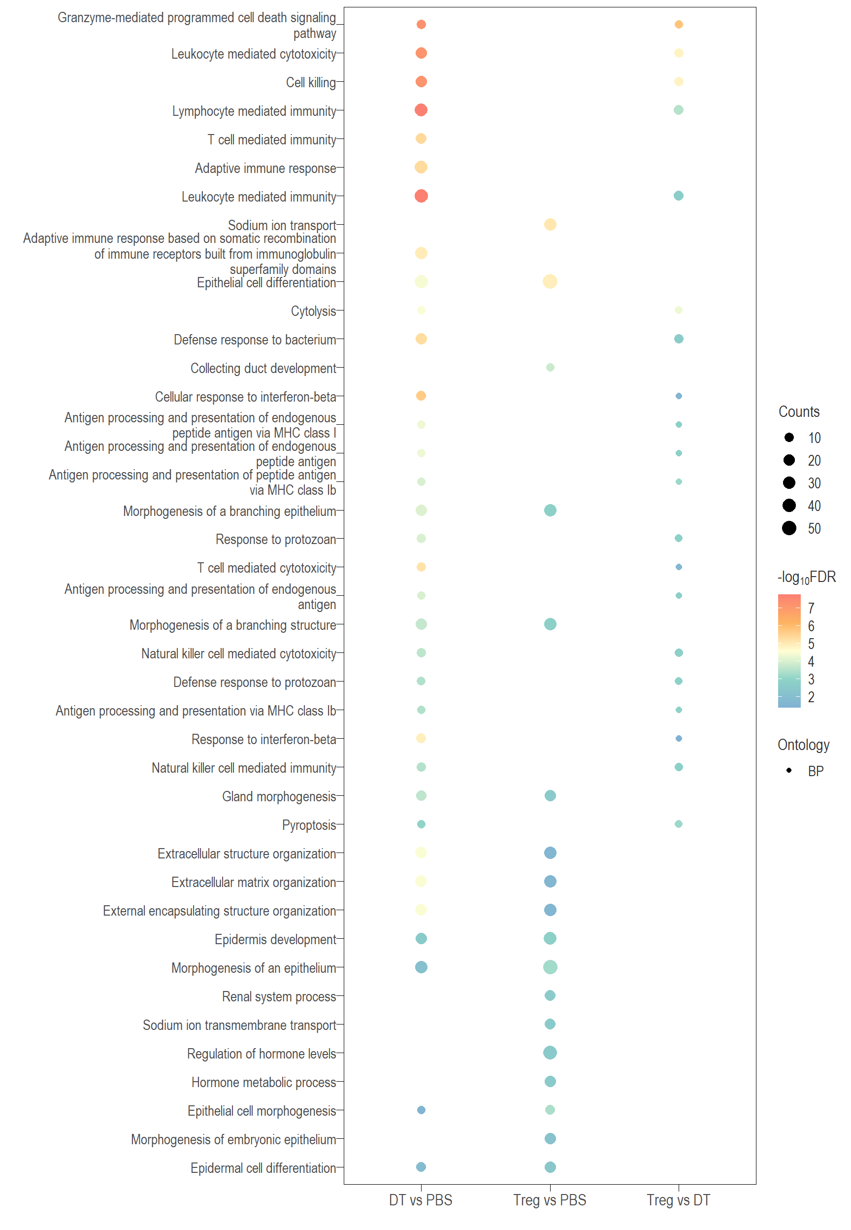
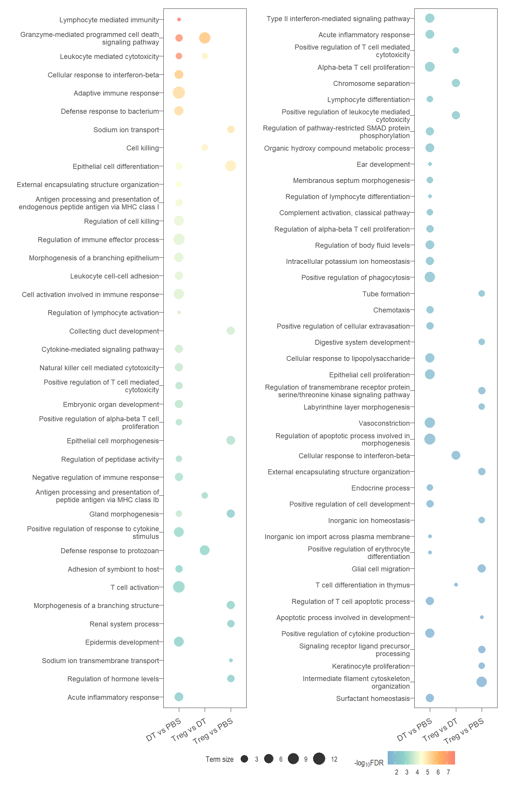
The following visualisations are GO enrichment analysis performed with set of DE genes significantly below FDR 0.1 without FC threshold (TREAT). IMPORTANTLY, these GO terms are all significantly enriched (FDR <0.05)
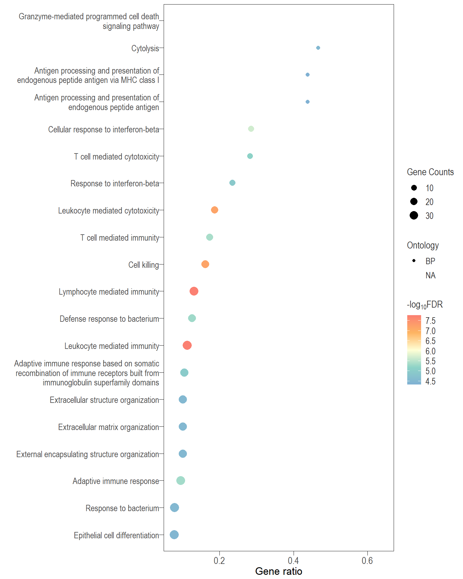
Dot plot: illustrates the top 25 enriched GO terms.
- \(Gene ratio =\) the number of significant DE gene in the term / the total of number of genes in the term. Indicated by the size
- The shapes represents the three main GO categories, either BP, MP, or CC
Table: list of all the significant GO terms
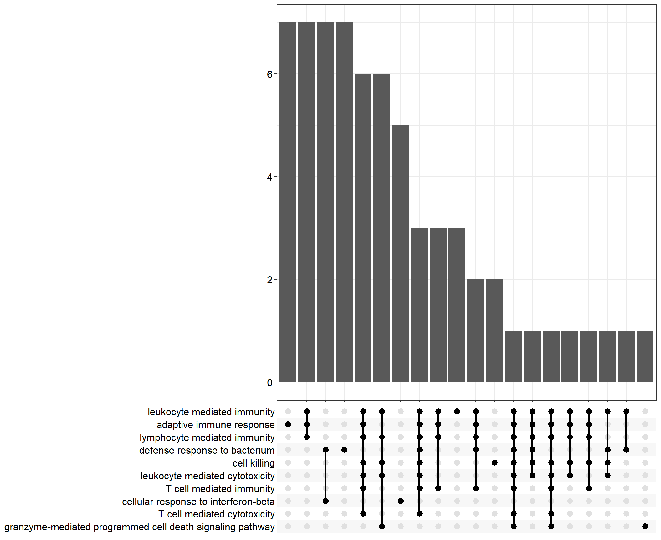
Upset: illustrate the overlap of gene between different functional terms
Semantic similarity plots - GO specific
Due to the hierarchical structure of Gene Ontologies, the enriched sets generated often exhibit redundancy and pose challenges in interpretation. The subsequent analyses and visualizations seek to alleviate this redundancy in GO sets by grouping comparable terms based on their semantic similarity. The underlying concept behind measuring semantic similarity is grounded in the idea that genes sharing similar functions should possess analogous annotation vocabulary and exhibit close relationships within the ontology structure.
NOTE: the following semantic similarity analyses are performed using Graph-based method (Wang et al. 2007)
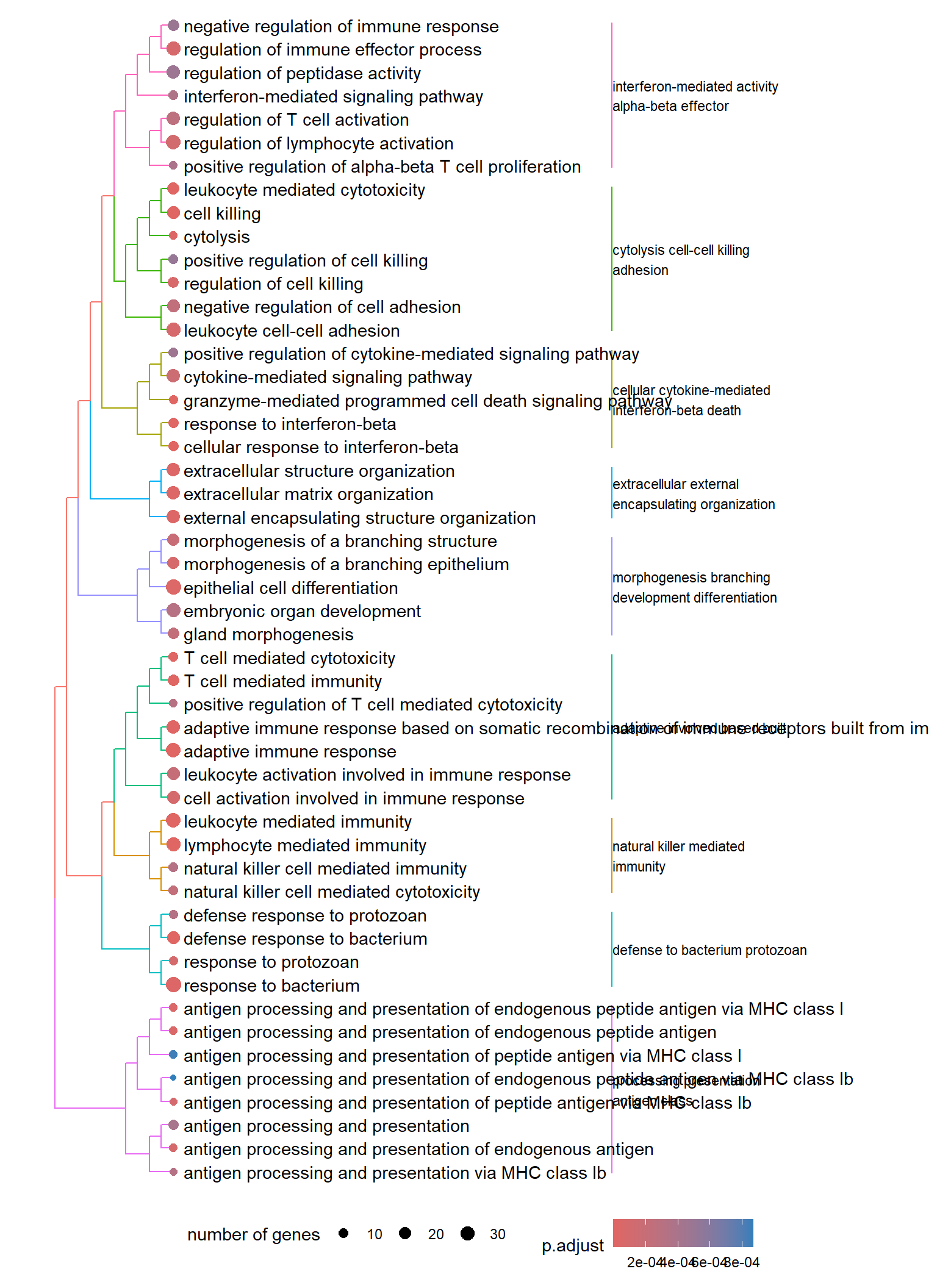
Dendrogram plot: performs hierarchical clustering on the semantic similarity of GO terms.
- NOTE: to maintain readability, only the top 50 most significant GO terms are clustered. These clusters are then divided into 9 clades and labeled using the top 4 high-frequency words.
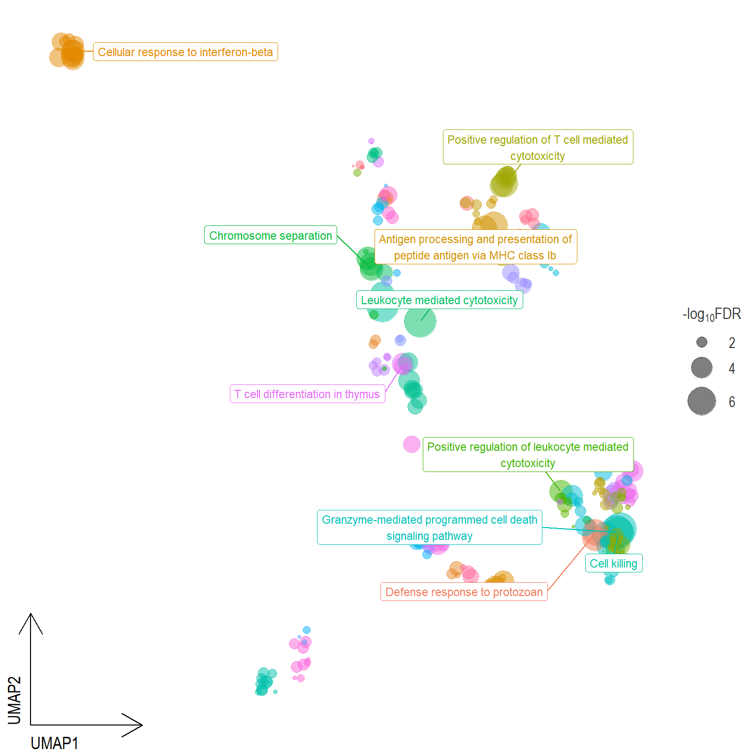
Scatter plot: illustrates the UMAP space between semantically similar significant GO terms
- Distances represent the similarity between terms,
- Size represents the significance (in \(-\log_{10}FDR\)))
- NOTE: to maintain reability, only the top 15 most significant parent terms are labeled. Parent terms are the most significant term in a particular cluster
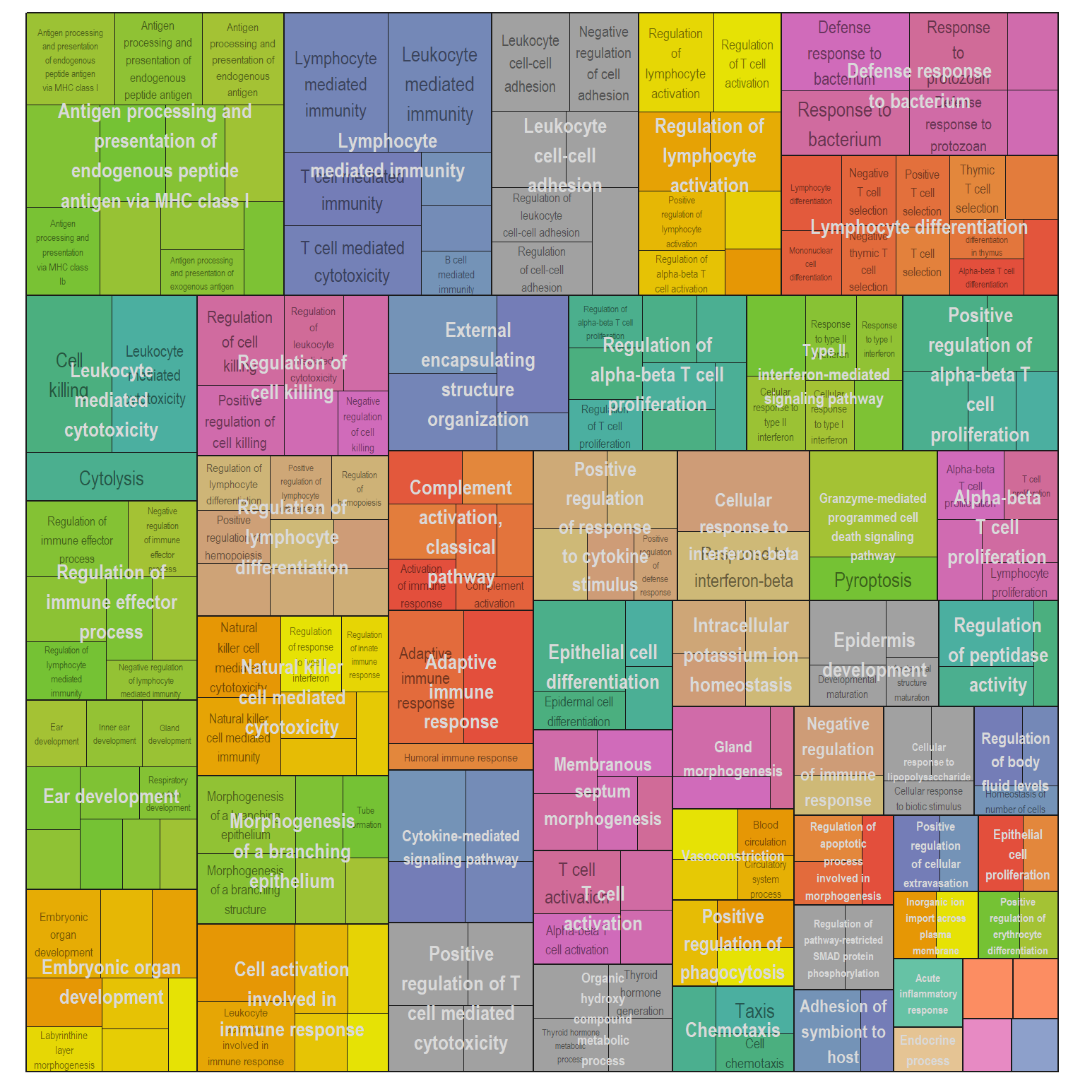
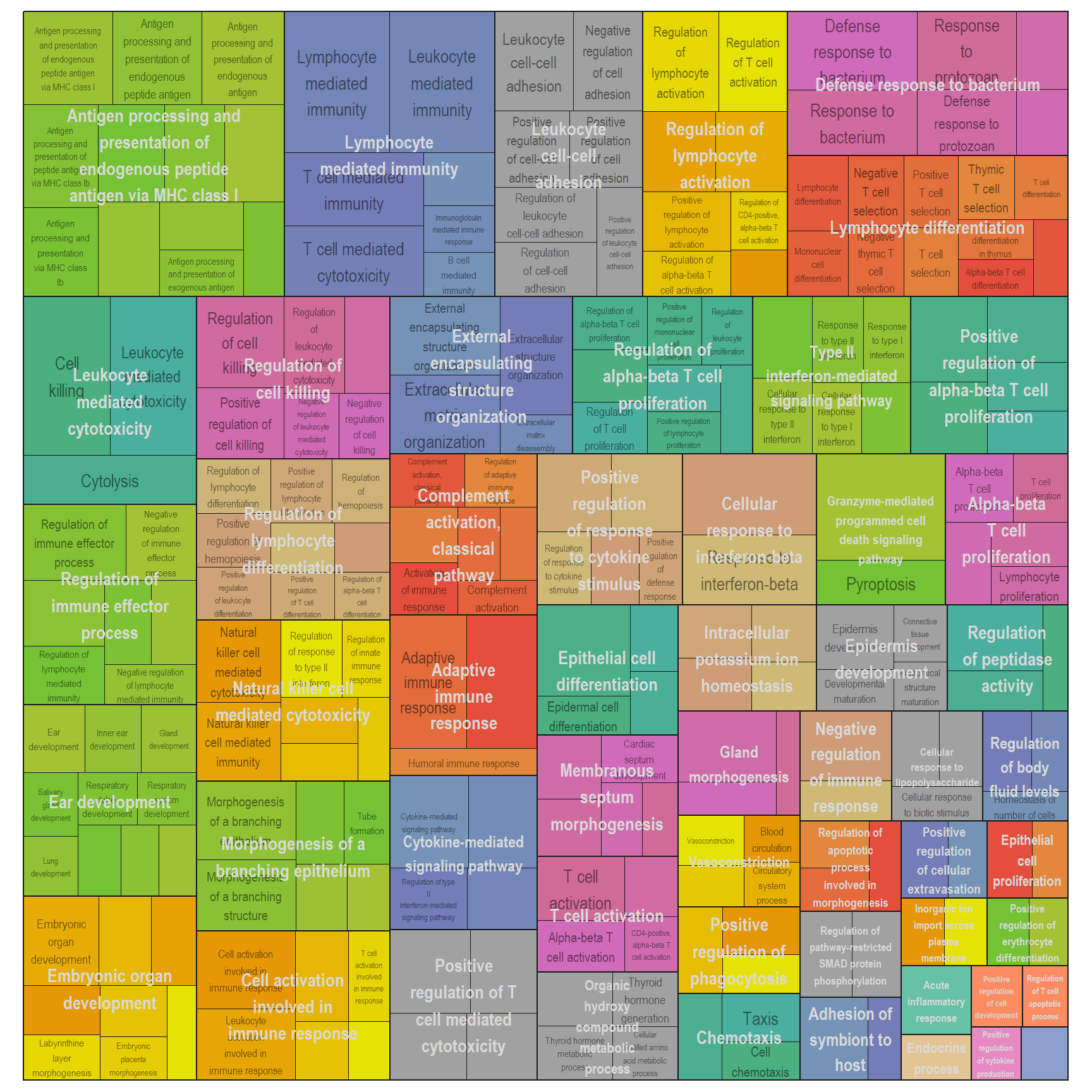
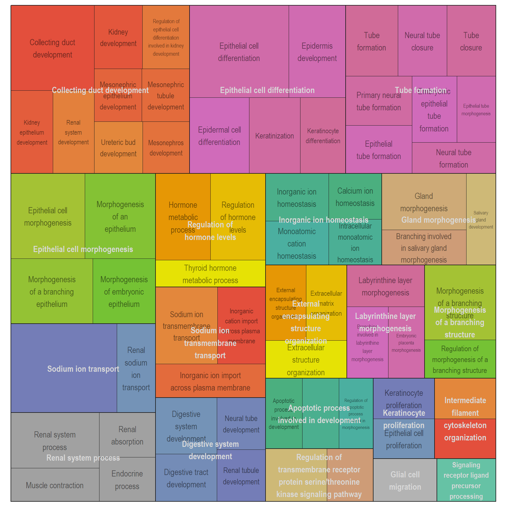
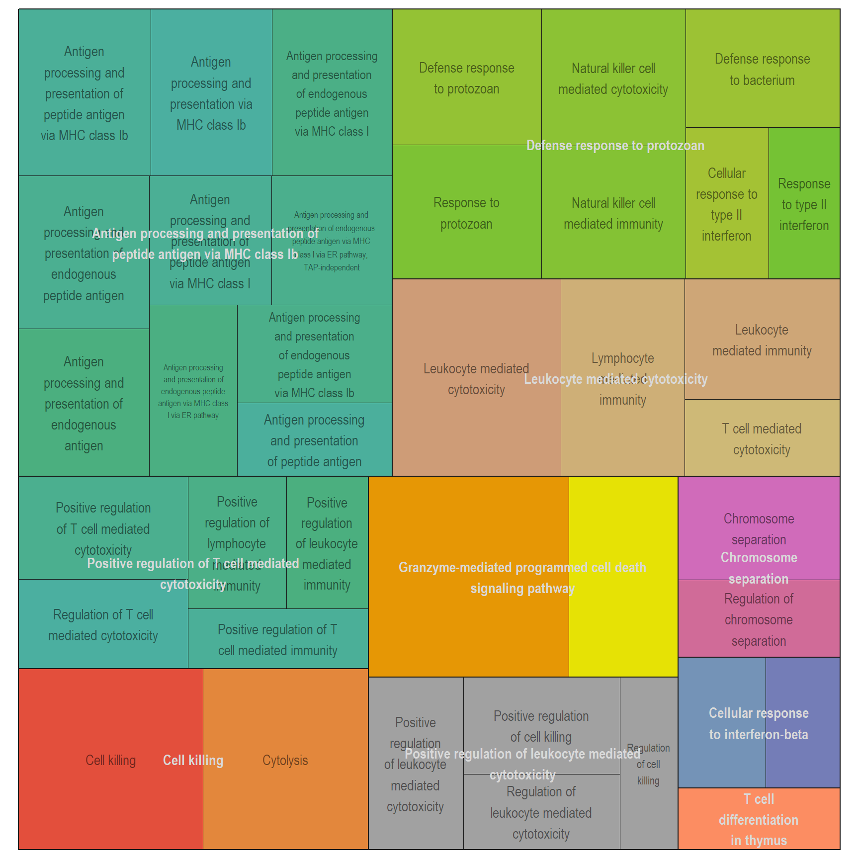
Treemap plot: Visualise the of hierarchical structures of semantically similar GO terms.
- The terms are colored based on their parent term,
- The size of the term is proportional to the significance.
I recommend reading through the full list of significant GO terms and selecting the most biologically relevant for better visualisation
DT vs PBS
Dot plot
Table
Upset plot
Dendrogram
Scatter plot
Interactive scatter
3D Interactive scatter
Parent terms
[[1]]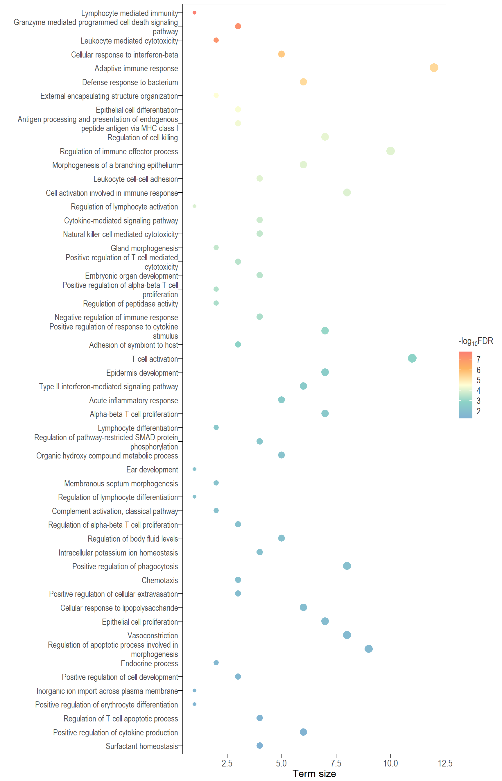
Treg vs PBS
Dot plot
.pl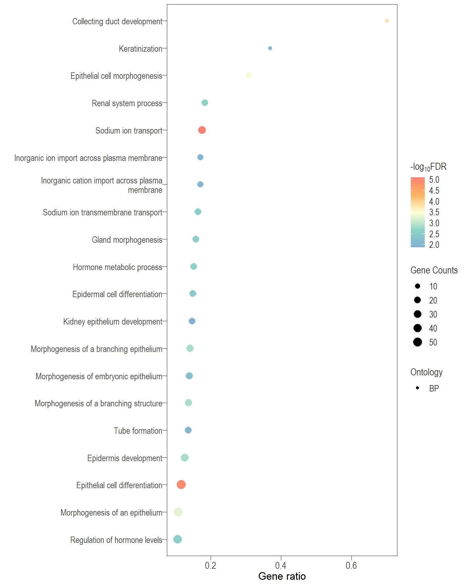
Table
.plUpset plot
.pl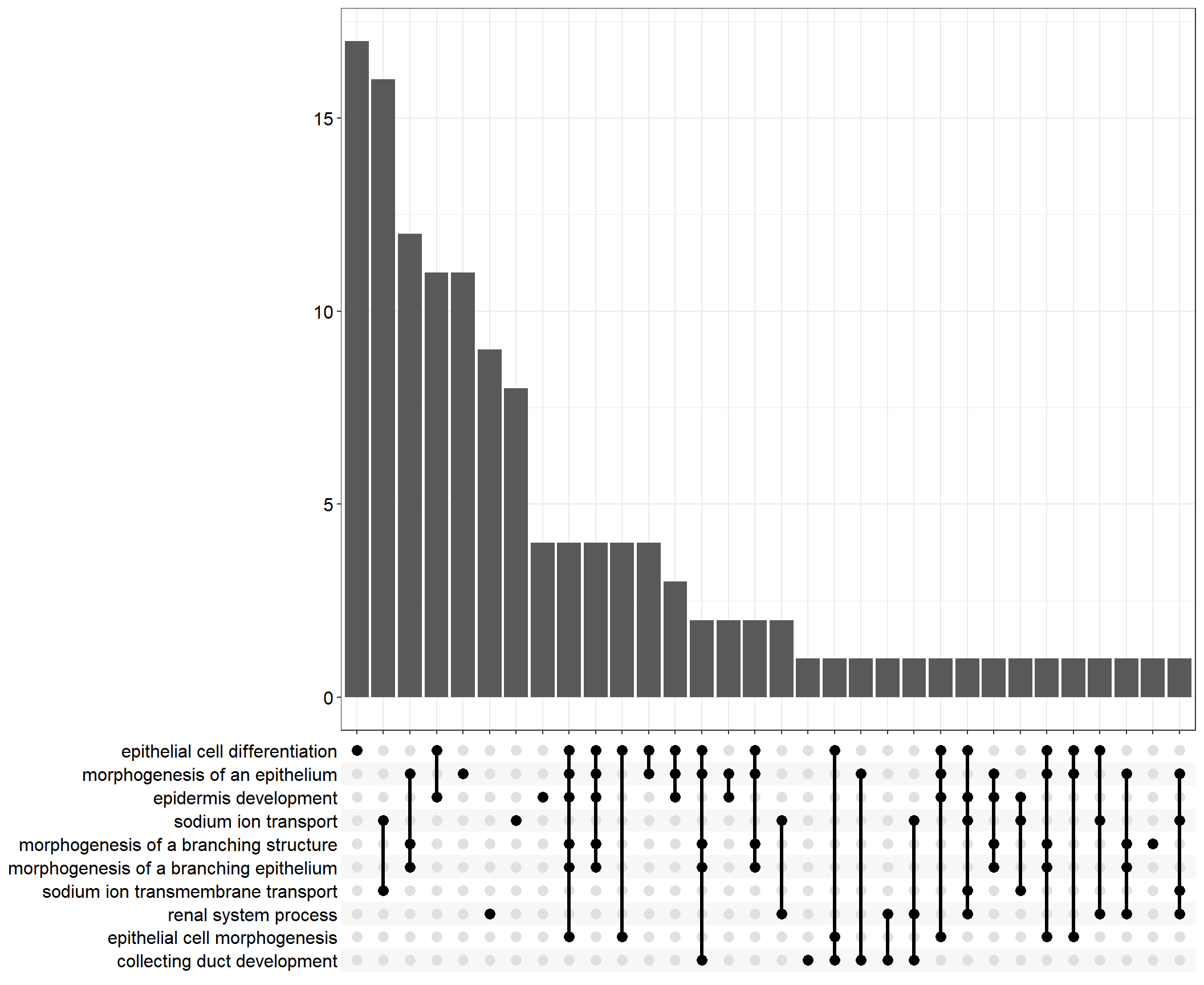
Dendrogram
.pl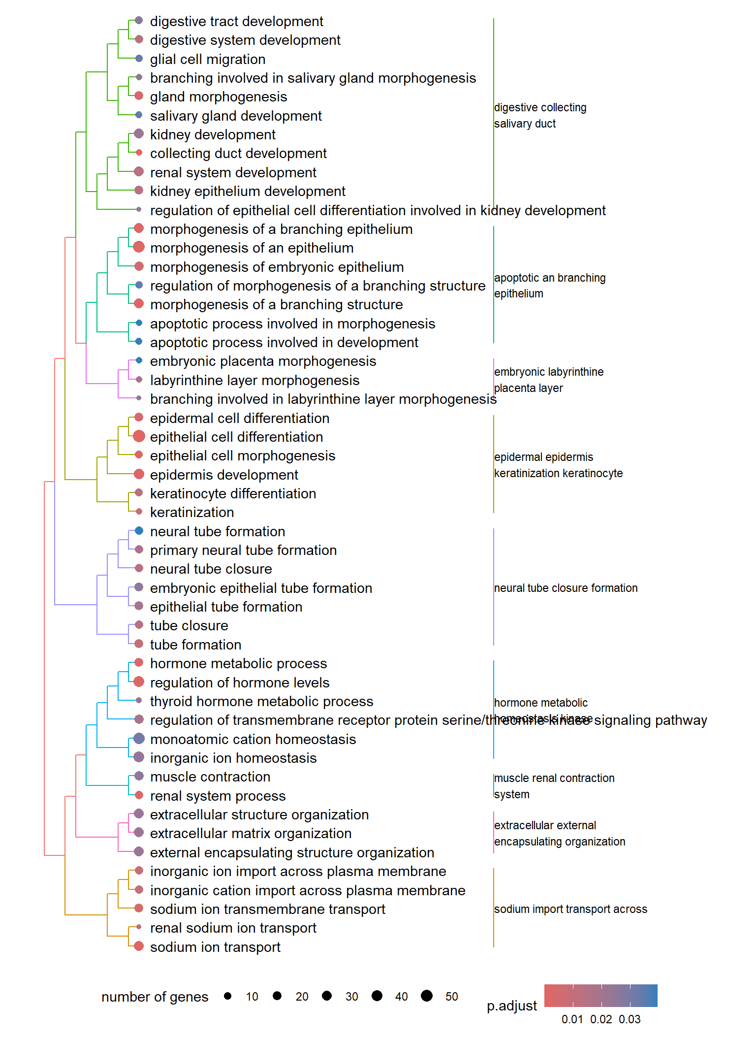
Scatter
.pl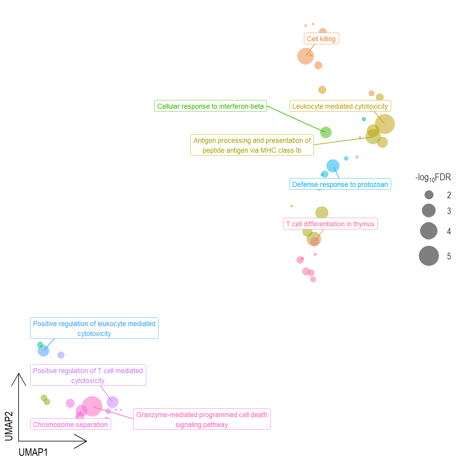
Interactive Scatter
.pl3D scatter
.plParent term
.pl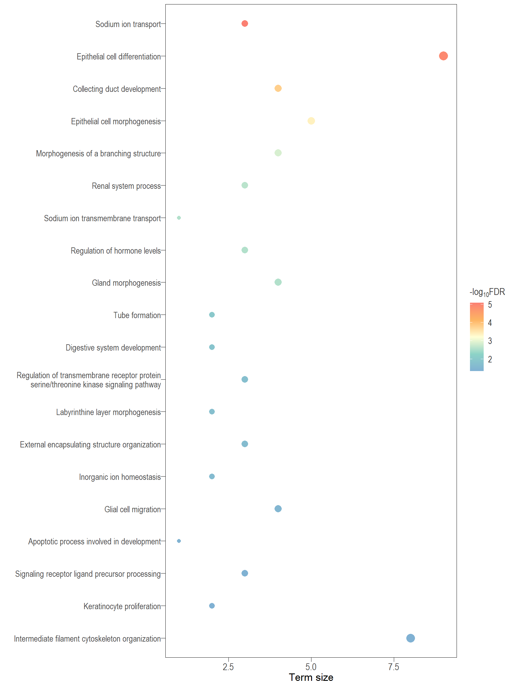
Treg vs DT
Dot plot
.pl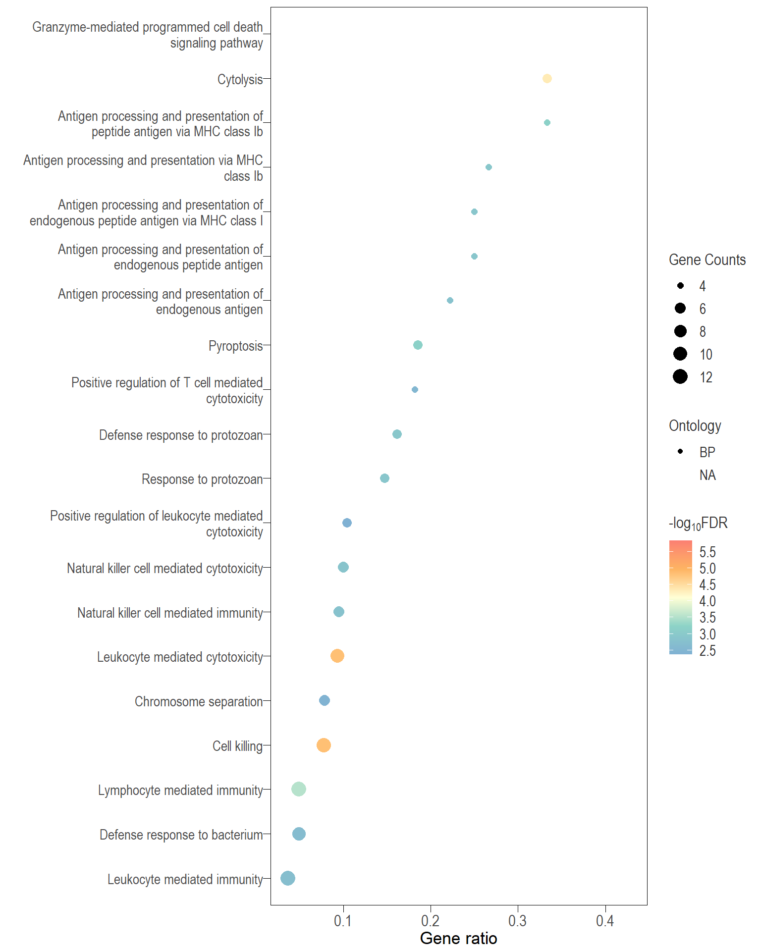
Table
.plUpset plot
.pl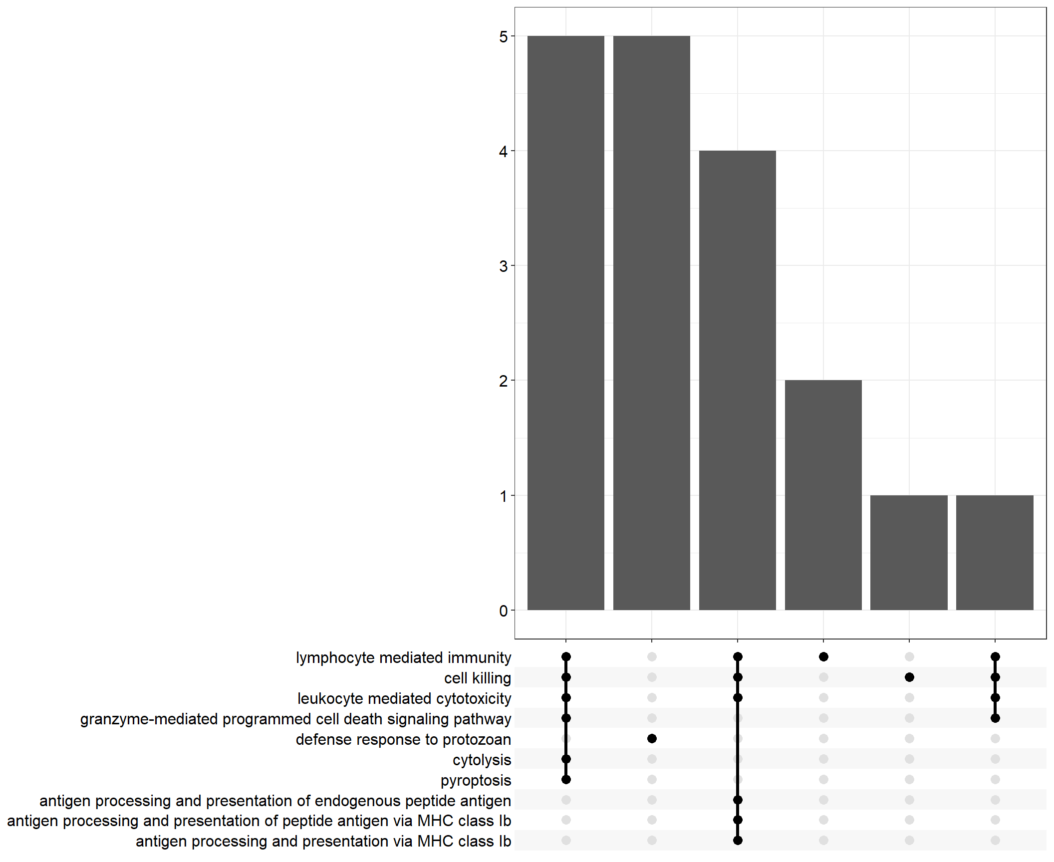
Dendrogram
.pl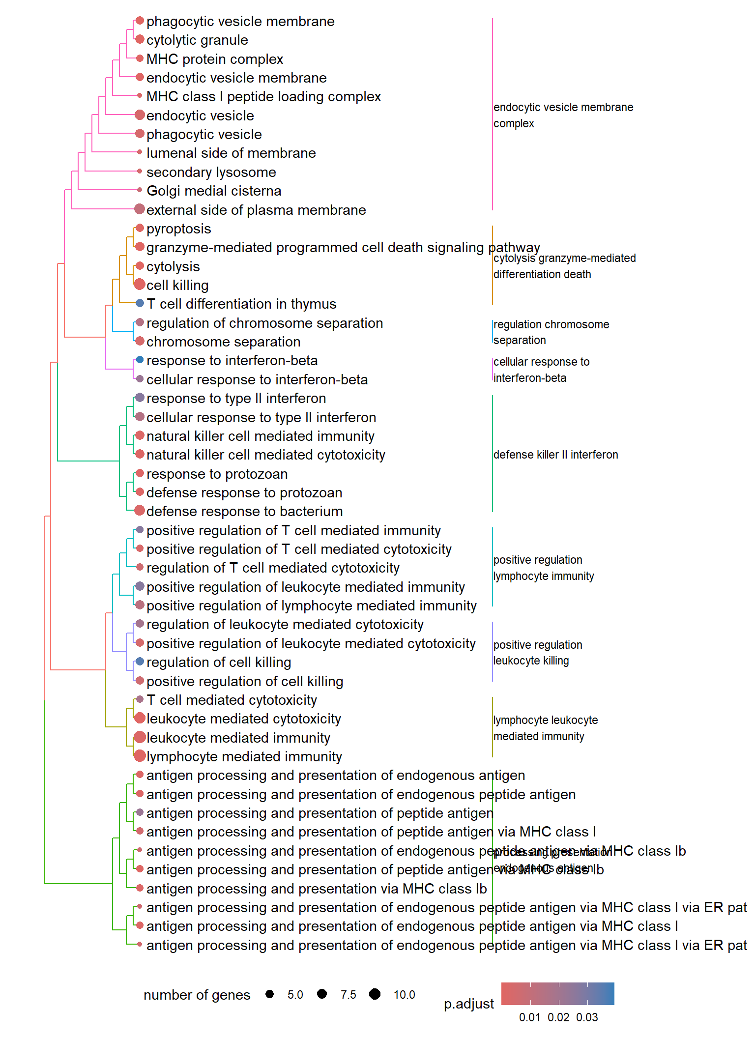
Scatter
.pl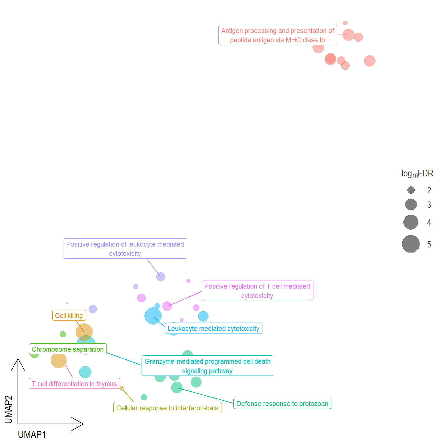
Interactive Scatter
.pl3D scatter
.plParent term
.pl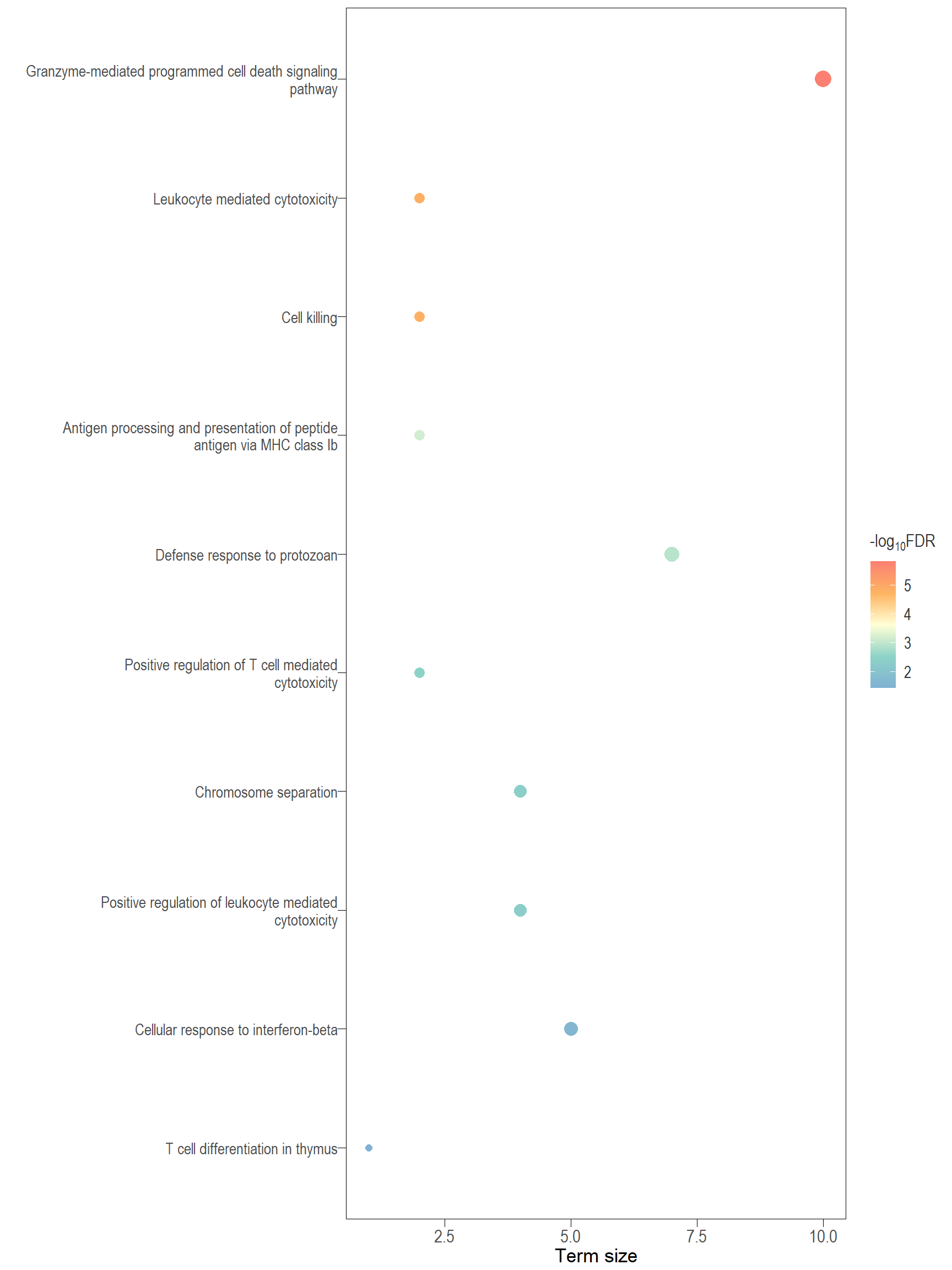
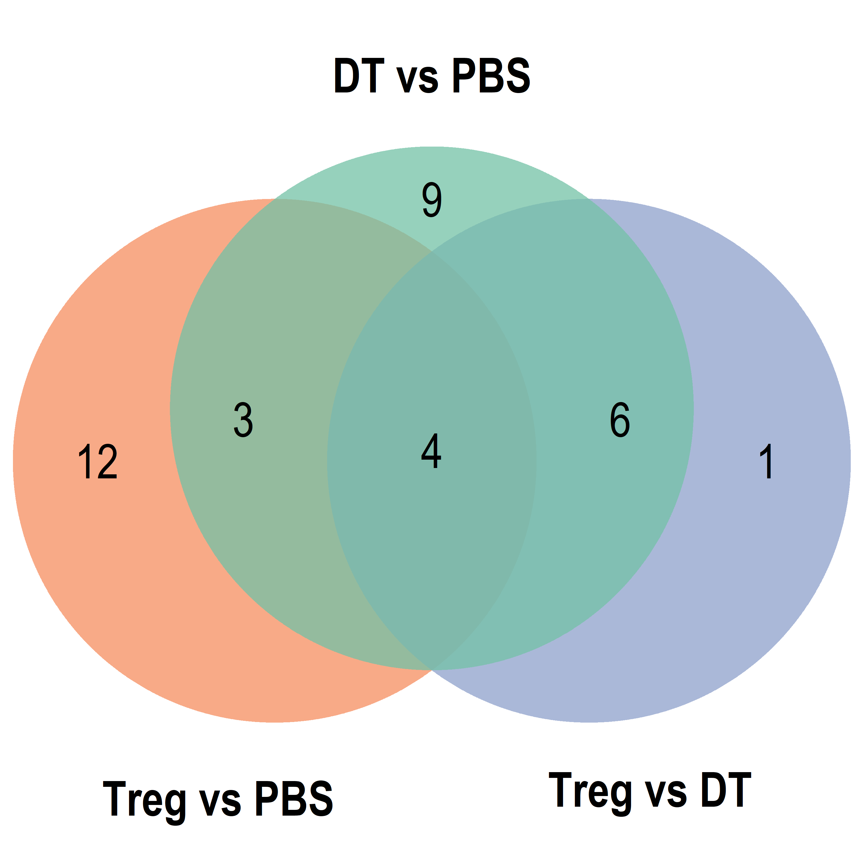
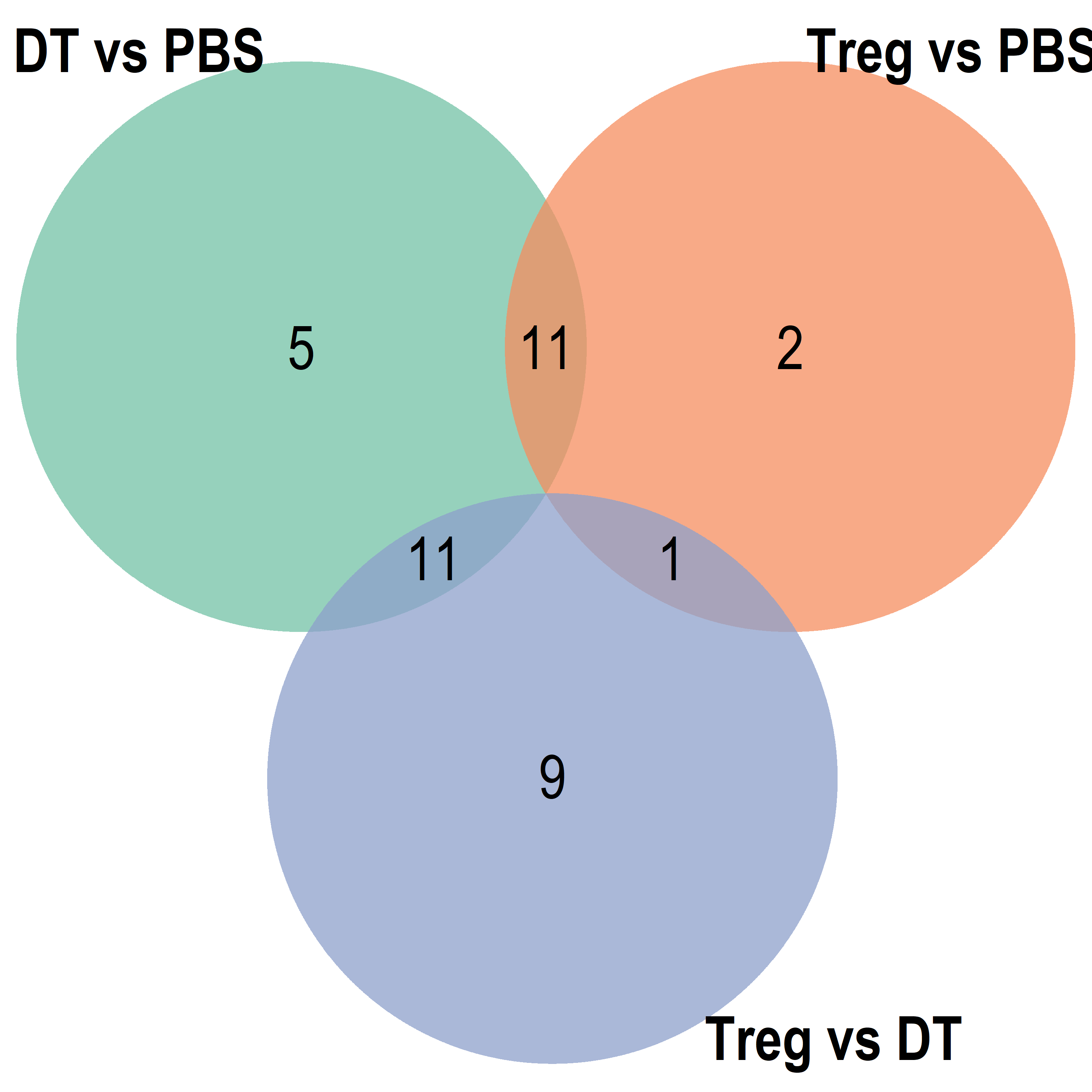
Combined
Venn diagram
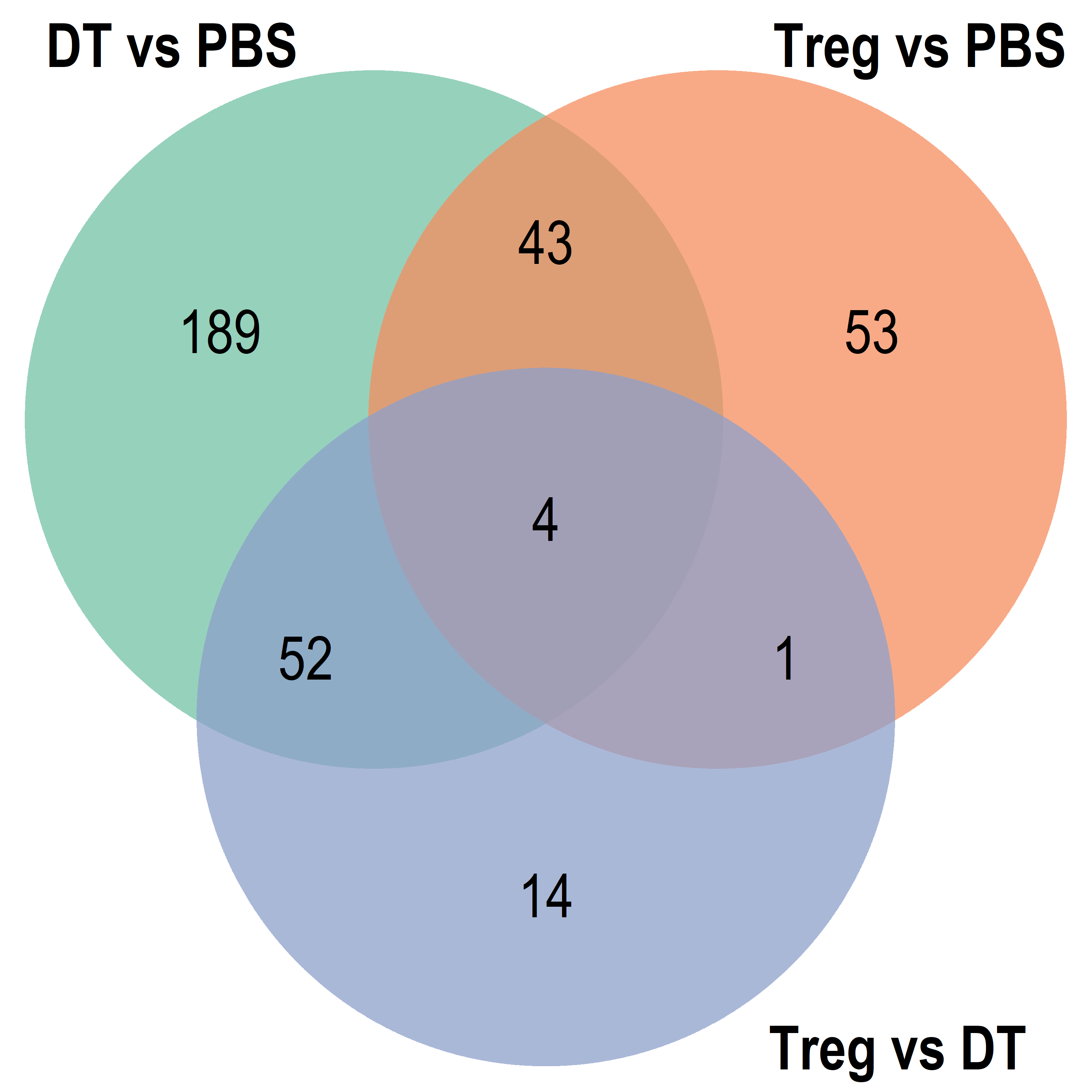
Parent term Venn
NULL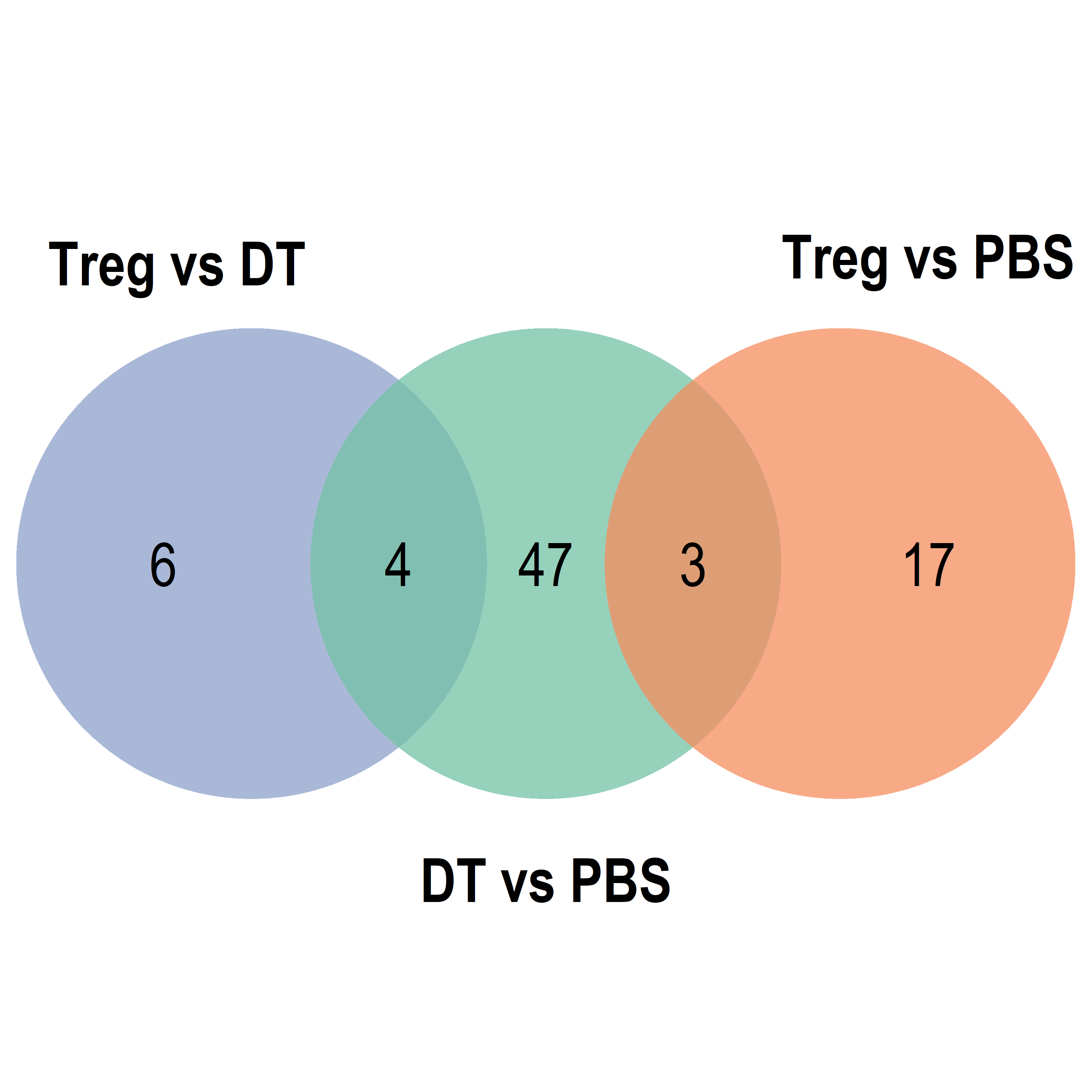
Export Data
The following are exported:
- GO.xlsx - This spreadsheet contains all significantly enriched GO terms. NOTE:
R version 4.3.1 (2023-06-16 ucrt)
Platform: x86_64-w64-mingw32/x64 (64-bit)
Running under: Windows 10 x64 (build 19045)

Matrix products: default


locale:
[1] LC_COLLATE=English_Australia.utf8  LC_CTYPE=English_Australia.utf8
[3] LC_MONETARY=English_Australia.utf8 LC_NUMERIC=C
[5] LC_TIME=English_Australia.utf8

time zone: Australia/Adelaide
tzcode source: internal

attached base packages:
[1] stats4    grid      stats     graphics  grDevices utils     datasets
[8] methods   base

other attached packages:
 [1] htmltools_0.5.7       knitr_1.45            pandoc_0.2.0
 [4] patchwork_1.1.3       enrichplot_1.20.3     org.Mm.eg.db_3.17.0
 [7] AnnotationDbi_1.62.2  IRanges_2.34.1        S4Vectors_0.38.2
[10] Biobase_2.60.0        BiocGenerics_0.46.0   clusterProfiler_4.8.3
[13] Glimma_2.10.0         edgeR_3.42.4          limma_3.56.2
[16] data.table_1.14.10    GOSemSim_2.26.1       plotly_4.10.3
[19] d3treeR_0.1           rrvgo_1.12.2          ggrepel_0.9.4
[22] ggbiplot_0.55         scales_1.3.0          plyr_1.8.9
[25] gridExtra_2.3         VennDiagram_1.7.3     futile.logger_1.4.3
[28] extrafont_0.19        DT_0.31               kableExtra_1.3.4
[31] lubridate_1.9.3       forcats_1.0.0         stringr_1.5.1
[34] purrr_1.0.2           tidyr_1.3.0           ggplot2_3.4.4
[37] tidyverse_2.0.0       reshape2_1.4.4        tibble_3.2.1
[40] readr_2.1.4           magrittr_2.0.3        dplyr_1.1.4

loaded via a namespace (and not attached):
  [1] splines_4.3.1               later_1.3.2
  [3] ggplotify_0.1.2             bitops_1.0-7
  [5] polyclip_1.10-6             XML_3.99-0.16
  [7] lifecycle_1.0.4             rprojroot_2.0.4
  [9] MASS_7.3-60                 NLP_0.2-1
 [11] lattice_0.21-8              crosstalk_1.2.1
 [13] sass_0.4.8                  rmarkdown_2.25
 [15] jquerylib_0.1.4             yaml_2.3.7
 [17] httpuv_1.6.13               askpass_1.2.0
 [19] reticulate_1.34.0           cowplot_1.1.2
 [21] DBI_1.2.0                   RColorBrewer_1.1-3
 [23] abind_1.4-5                 zlibbioc_1.46.0
 [25] rvest_1.0.3                 GenomicRanges_1.52.1
 [27] ggraph_2.1.0                RCurl_1.98-1.13
 [29] yulab.utils_0.1.1           rappdirs_0.3.3
 [31] tweenr_2.0.2                git2r_0.33.0
 [33] GenomeInfoDbData_1.2.10     data.tree_1.1.0
 [35] tm_0.7-11                   tidytree_0.4.6
 [37] pheatmap_1.0.12             umap_0.2.10.0
 [39] RSpectra_0.16-1             svglite_2.1.3
 [41] gridSVG_1.7-5               codetools_0.2-19
 [43] DelayedArray_0.26.7         ggforce_0.4.1
 [45] DOSE_3.26.2                 xml2_1.3.6
 [47] tidyselect_1.2.0            aplot_0.2.2
 [49] farver_2.1.1                viridis_0.6.4
 [51] matrixStats_1.2.0           webshot_0.5.5
 [53] jsonlite_1.8.8              ellipsis_0.3.2
 [55] tidygraph_1.3.0             systemfonts_1.0.5
 [57] ggnewscale_0.4.9            tools_4.3.1
 [59] treeio_1.24.3               Rcpp_1.0.11
 [61] glue_1.6.2                  Rttf2pt1_1.3.12
 [63] here_1.0.1                  xfun_0.39
 [65] DESeq2_1.40.2               qvalue_2.32.0
 [67] MatrixGenerics_1.12.3       GenomeInfoDb_1.36.4
 [69] withr_2.5.2                 formatR_1.14
 [71] fastmap_1.1.1               ggh4x_0.2.7
 [73] fansi_1.0.6                 openssl_2.1.1
 [75] digest_0.6.33               gridGraphics_0.5-1
 [77] timechange_0.2.0            R6_2.5.1
 [79] mime_0.12                   colorspace_2.1-0
 [81] GO.db_3.17.0                RSQLite_2.3.4
 [83] utf8_1.2.4                  generics_0.1.3
 [85] graphlayouts_1.0.2          httr_1.4.7
 [87] htmlwidgets_1.6.4           S4Arrays_1.0.6
 [89] scatterpie_0.2.1            whisker_0.4.1
 [91] pkgconfig_2.0.3             gtable_0.3.4
 [93] blob_1.2.4                  workflowr_1.7.1
 [95] XVector_0.40.0              shadowtext_0.1.2
 [97] fgsea_1.26.0                ggupset_0.3.0
 [99] png_0.1-8                   wordcloud_2.6
[101] ggfun_0.1.3                 lambda.r_1.2.4
[103] rstudioapi_0.15.0           tzdb_0.4.0
[105] nlme_3.1-164                cachem_1.0.8
[107] parallel_4.3.1              HDO.db_0.99.1
[109] treemap_2.4-4               pillar_1.9.0
[111] vctrs_0.6.5                 slam_0.1-50
[113] promises_1.2.1              xtable_1.8-4
[115] extrafontdb_1.0             evaluate_0.23
[117] cli_3.6.1                   locfit_1.5-9.8
[119] compiler_4.3.1              futile.options_1.0.1
[121] rlang_1.1.1                 crayon_1.5.2
[123] labeling_0.4.3              fs_1.6.3
[125] stringi_1.8.3               viridisLite_0.4.2
[127] gridBase_0.4-7              BiocParallel_1.34.2
[129] munsell_0.5.0               Biostrings_2.68.1
[131] lazyeval_0.2.2              Matrix_1.6-4
[133] hms_1.1.3                   bit64_4.0.5
[135] KEGGREST_1.40.1             shiny_1.8.0
[137] highr_0.10                  SummarizedExperiment_1.30.2
[139] igraph_1.6.0                memoise_2.0.1
[141] bslib_0.6.1                 ggtree_3.8.2
[143] fastmatch_1.1-4             bit_4.0.5
[145] downloader_0.4              gson_0.1.0
[147] ape_5.7-1