Map Creation
Troy Rowan
2020-07-09
Last updated: 2020-07-10
Checks: 7 0
Knit directory: local_adaptation_sequence/
This reproducible R Markdown analysis was created with workflowr (version 1.6.2). The Checks tab describes the reproducibility checks that were applied when the results were created. The Past versions tab lists the development history.
Great! Since the R Markdown file has been committed to the Git repository, you know the exact version of the code that produced these results.
Great job! The global environment was empty. Objects defined in the global environment can affect the analysis in your R Markdown file in unknown ways. For reproduciblity it’s best to always run the code in an empty environment.
The command set.seed(20200709) was run prior to running the code in the R Markdown file. Setting a seed ensures that any results that rely on randomness, e.g. subsampling or permutations, are reproducible.
Great job! Recording the operating system, R version, and package versions is critical for reproducibility.
Nice! There were no cached chunks for this analysis, so you can be confident that you successfully produced the results during this run.
Great job! Using relative paths to the files within your workflowr project makes it easier to run your code on other machines.
Great! You are using Git for version control. Tracking code development and connecting the code version to the results is critical for reproducibility.
The results in this page were generated with repository version ff7fd0f. See the Past versions tab to see a history of the changes made to the R Markdown and HTML files.
Note that you need to be careful to ensure that all relevant files for the analysis have been committed to Git prior to generating the results (you can use wflow_publish or wflow_git_commit). workflowr only checks the R Markdown file, but you know if there are other scripts or data files that it depends on. Below is the status of the Git repository when the results were generated:
Ignored files:
    Ignored:    .Rhistory
    Ignored:    .Rproj.user/

Untracked files:
    Untracked:  data/PRISM_ppt_30yr_normal_4kmM2_annual_asc.asc
    Untracked:  data/prism_climate_data/
    Untracked:  desktop.ini
    Untracked:  output/desktop.ini
    Untracked:  output/kmeans_plotlist.RDS
Note that any generated files, e.g. HTML, png, CSS, etc., are not included in this status report because it is ok for generated content to have uncommitted changes.
These are the previous versions of the repository in which changes were made to the R Markdown (analysis/map_making.Rmd) and HTML (docs/map_making.html) files. If you’ve configured a remote Git repository (see ?wflow_git_remote), click on the hyperlinks in the table below to view the files as they were in that past version.
| File | Version | Author | Date | Message |
|---|---|---|---|---|
| Rmd | ff7fd0f | Troy Rowan | 2020-07-10 | Checking to see if tabs work for maps on website now |
| html | ae01f68 | Troy Rowan | 2020-07-10 | Build site. |
| Rmd | 5dad063 | Troy Rowan | 2020-07-10 | Fixed tabset plotting for kmeans maps |
| html | d64c6ee | Troy Rowan | 2020-07-10 | Build site. |
| Rmd | 897d00b | Troy Rowan | 2020-07-10 | Fixed link |
| html | d2da211 | Troy Rowan | 2020-07-10 | Build site. |
| Rmd | c205415 | Troy Rowan | 2020-07-10 | Extensive reworking to make initial website with maps example |
| Rmd | a2d16f5 | Troy Rowan | 2020-07-09 | Added page for map making and starte exploring k-means approach |
Introduction
This uses k-means clustering and 30-year normal climate variables to divide the United States into distinct ecoregions.
Reading in climate raster files
These originate from the Prism Climate Group’s website in .bil format I was having issues with the rgdal package reading these or any other form, so had to read them and save as RDS files on Workstation (the only place where rgdal installs properly). SCP’d RDS files here, and these read in the individal environment variable rasters.
temp_raster =
  readRDS(
    here::here("data", "prism_climate_data", "temp_raster.RDS"))

precip_raster =
  readRDS(
    here::here("data", "prism_climate_data", "precip_raster.RDS"))

elev_raster =
  readRDS(
    here::here("data", "prism_climate_data", "elev_raster.RDS"))

dewpt_raster =
  readRDS(
    here::here("data", "prism_climate_data", "mean_dwpt_raster.RDS")
  )

min_vap_raster =
  readRDS(
    here::here("data", "prism_climate_data", "min_vpd_raster.RDS"))

max_vap_raster =
  readRDS(
    here::here("data", "prism_climate_data", "max_vpd_raster.RDS"))

min_temp_raster =
  readRDS(
    here::here("data", "prism_climate_data", "min_temp_raster.RDS"))

max_temp_raster =
  readRDS(
    here::here("data", "prism_climate_data", "max_temp_raster.RDS"))
stacked_raster =
stack(
temp_raster,
precip_raster,
elev_raster,
dewpt_raster,
max_temp_raster,
min_temp_raster,
max_vap_raster,
min_vap_raster
)
threevar_stacked_raster =
stack(
temp_raster,
precip_raster,
elev_raster
)Identifying best K for full- and three-variable datasets
Using fpc::pamk(), K between 3 and 10 This doesn’t run, but appears that based on the fviz_nbclust() function in that the appropriate
It appears that k=2 is optimal by these metrics, but for some reason this step exceeds memory necessary to add to website.
stacked_raster %>%
  as.data.frame() %>%
  na.omit() %>%
  sample_n(20000) %>%
  fviz_nbclust(FUNcluster = kmeans)+
  ggtitle("Full Environmental Data")
  #pamk(krange = 3:20, criterion="multiasw", usepam=FALSE, scaling=TRUE)

threevar_stacked_raster %>%
  as.data.frame() %>%
  na.omit() %>%
  sample_n(20000) %>%
  fviz_nbclust(FUNcluster = kmeans)+
  ggtitle("Three Environmental Variables ")
  #pamk(krange = 3:20, criterion="multiasw", usepam=FALSE, scaling=TRUE)
K-means clustering climate maps
# plotlist =
#   seq(2,10) %>%
#   purrr::map(
#   ~plot_grid(
#     unsuperClass(stacked_raster,
#                nSamples=1000,
#                nClasses = .x,
#                norm=TRUE,
#                nStarts=5,
#                clusterMap=FALSE) %>%
#     .$map %>%
#     as.data.frame(xy=TRUE) %>%
#     mutate(layer = as.factor(layer)) %>%
#     kmeans_map()+
#       ggtitle(paste("All Variables, k =", .x)),
#     unsuperClass(threevar_stacked_raster,
#                  nSamples=1000,
#                  nClasses = .x,
#                  norm=TRUE,
#                  nStarts=5,
#                  clusterMap=FALSE) %>%
#     .$map %>%
#     as.data.frame(xy=TRUE) %>%
#     mutate(layer = as.factor(layer)) %>%
#     kmeans_map()+
#       ggtitle(paste("Three Variables, k =", .x))
#     )
#   )
#
# saveRDS(plotlist, "../output/kmeans_plotlist.RDS")

plotlist = readRDS(here::here("output", "kmeans_plotlist.RDS"))

for (i in 1:length(plotlist)){
  cat("###", i, " \n")
  print(plotlist[[i]])
  cat(' \n\n')
}
### 1 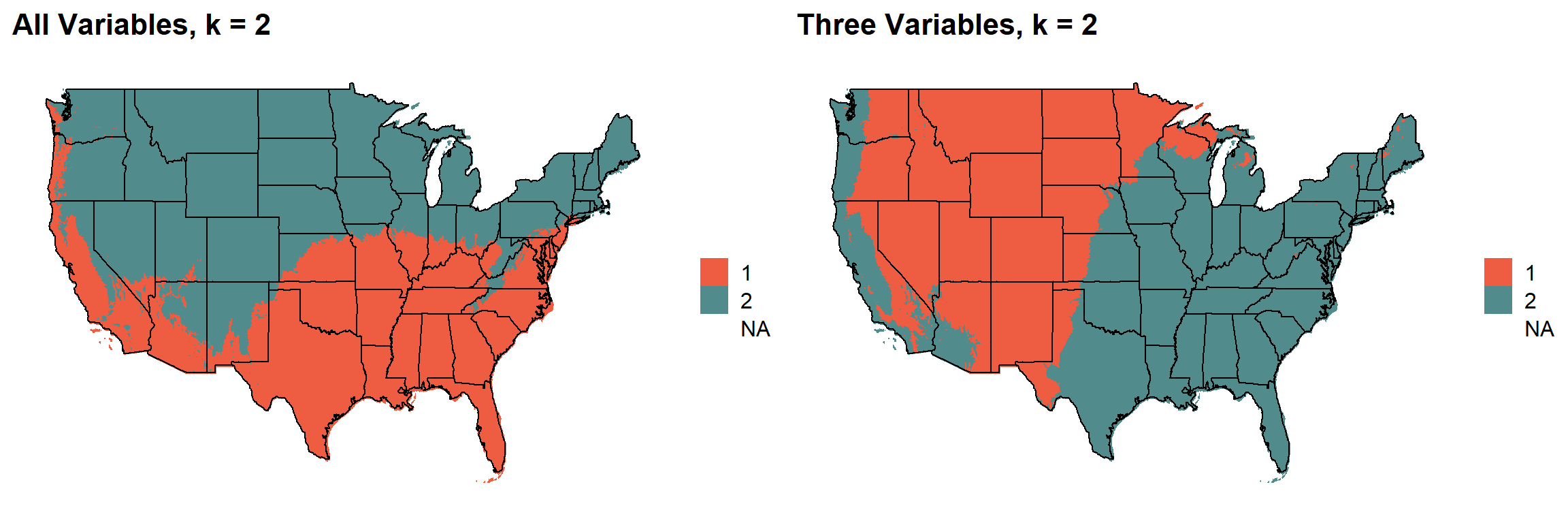
### 2 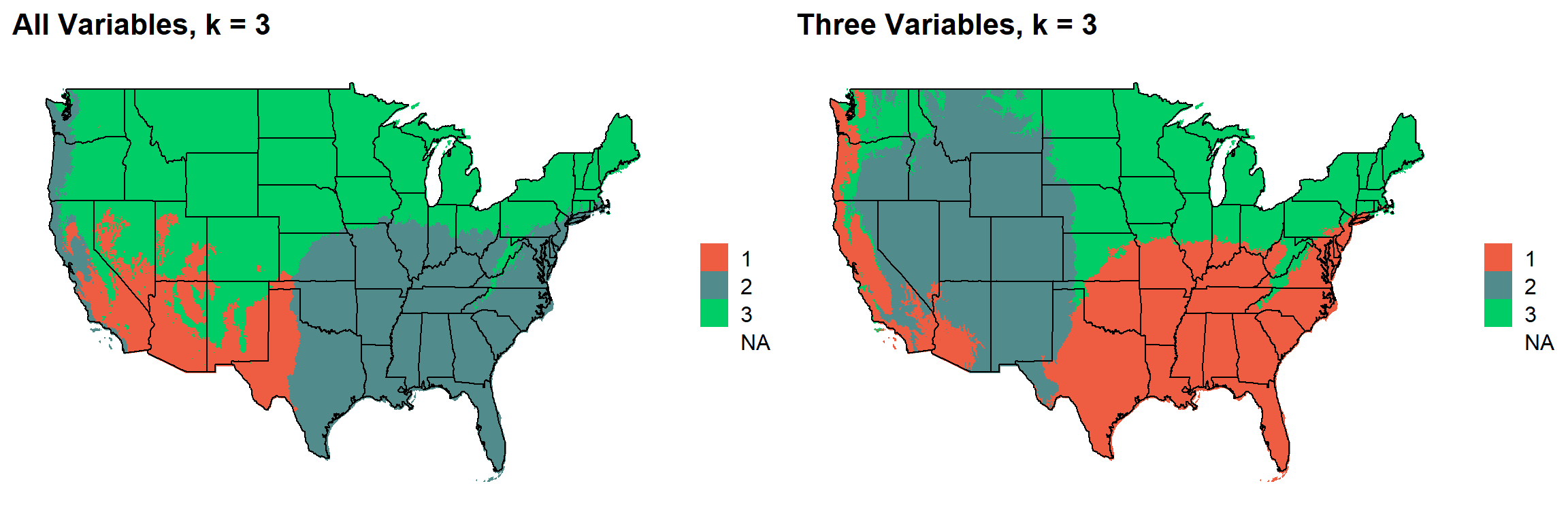
### 3 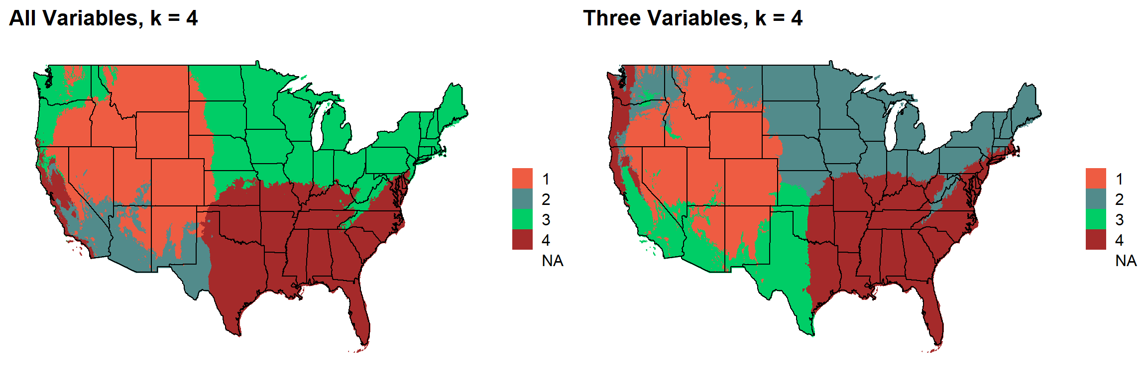
### 4 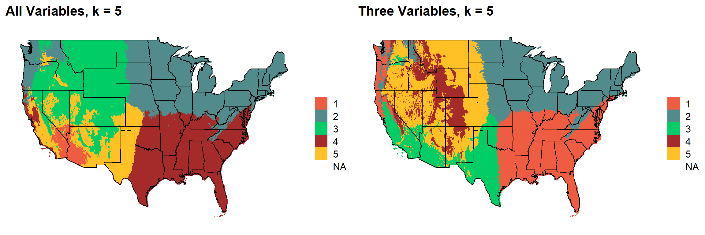
### 5 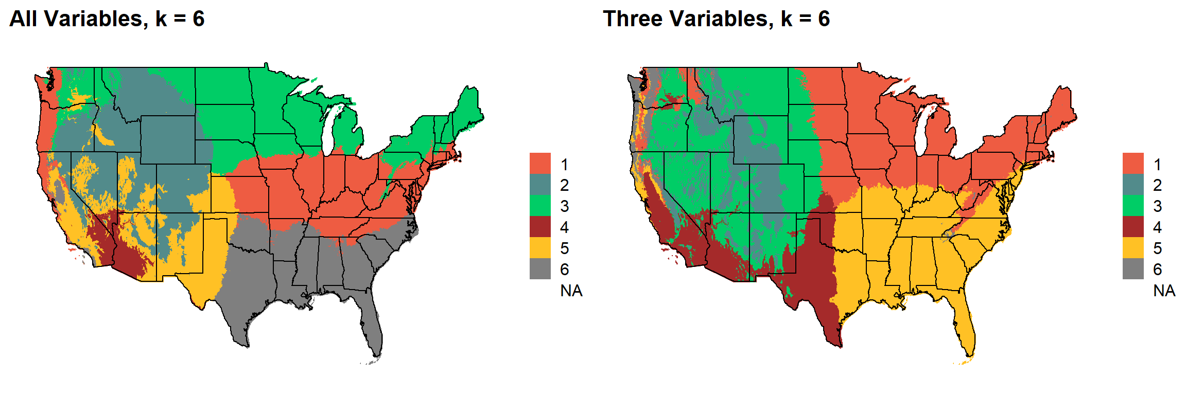
### 6 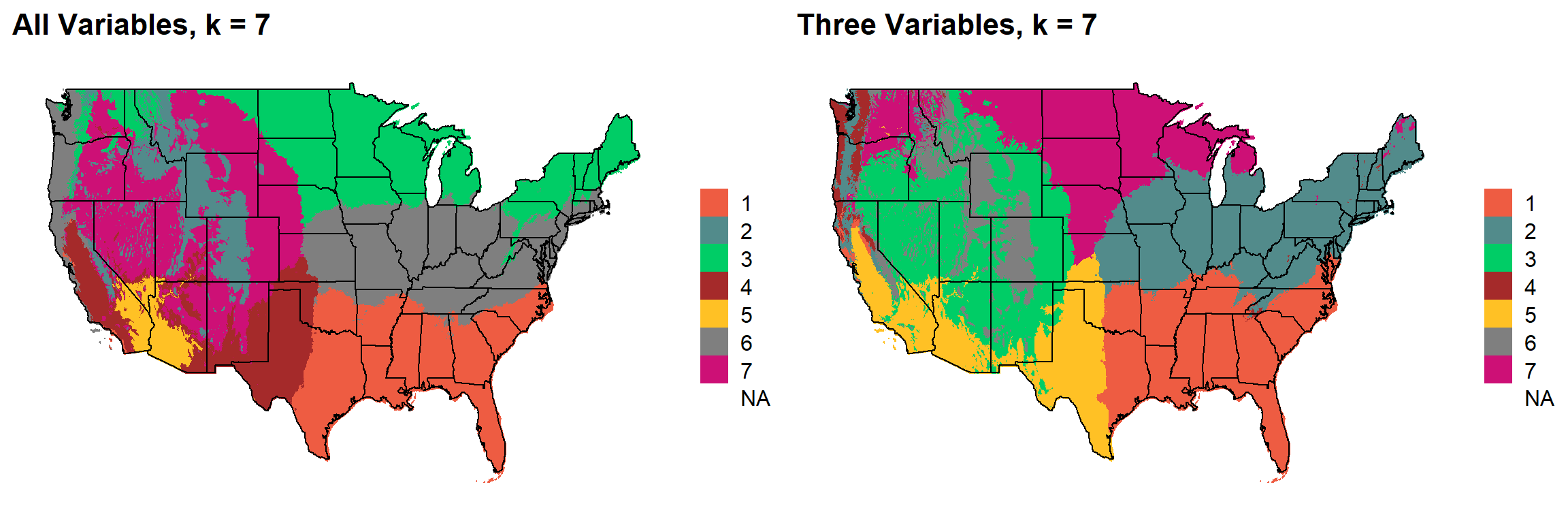
### 7 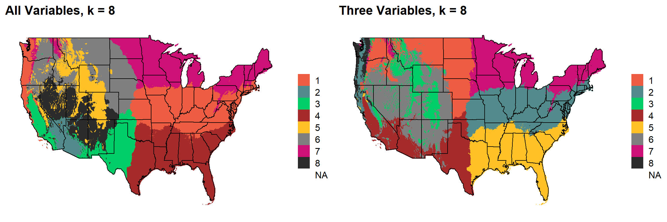
### 8 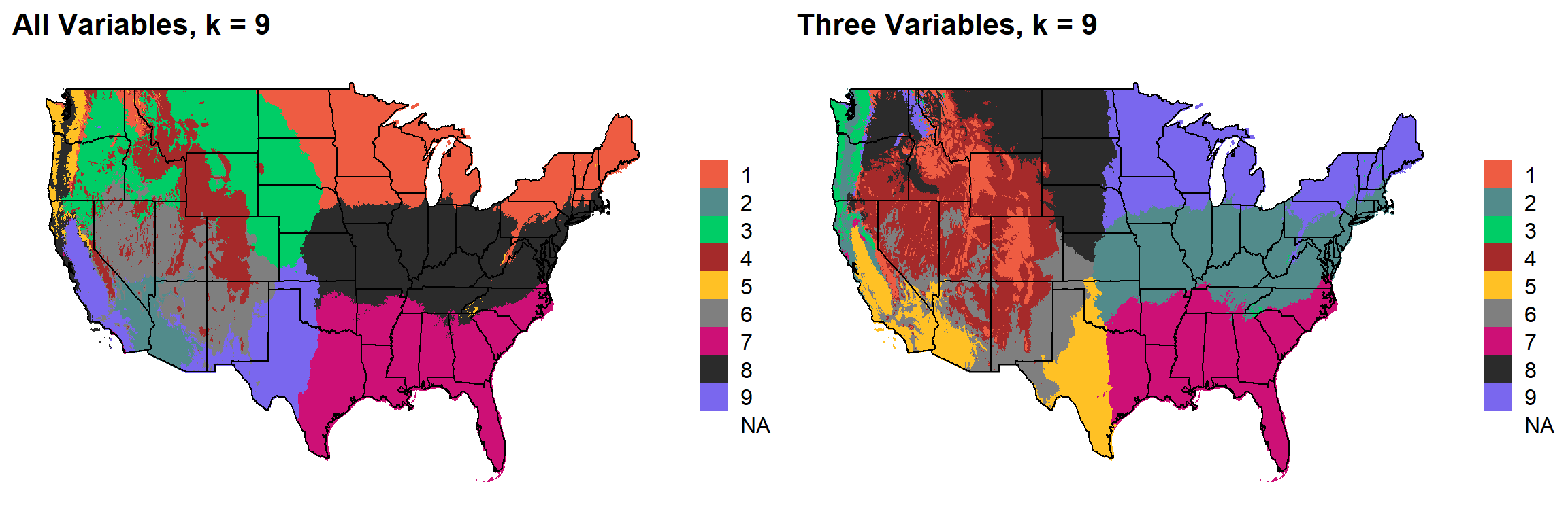
### 9 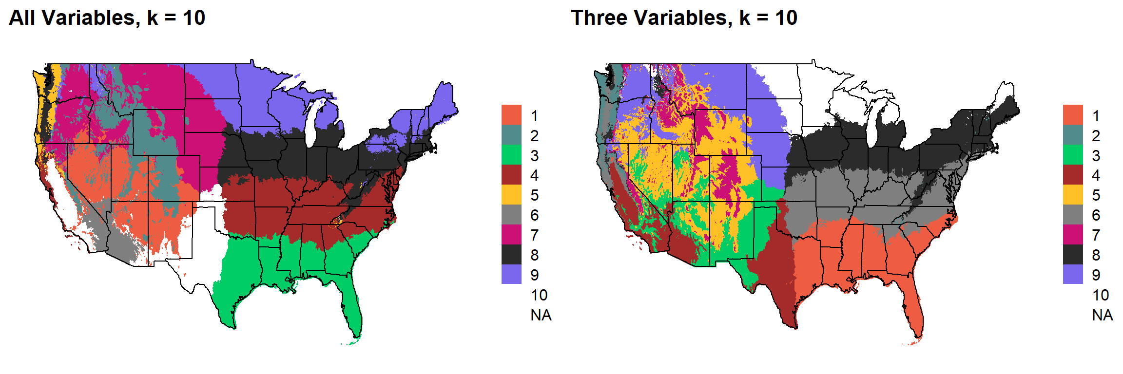
sessionInfo()R version 3.6.1 (2019-07-05)
Platform: x86_64-w64-mingw32/x64 (64-bit)
Running under: Windows 10 x64 (build 19041)
Matrix products: default
locale:
[1] LC_COLLATE=English_United States.1252
[2] LC_CTYPE=English_United States.1252
[3] LC_MONETARY=English_United States.1252
[4] LC_NUMERIC=C
[5] LC_TIME=English_United States.1252
attached base packages:
[1] stats graphics grDevices utils datasets methods base
other attached packages:
[1] factoextra_1.0.7 cowplot_1.0.0 ggthemes_4.2.0 maps_3.3.0
[5] RStoolbox_0.2.6 fpc_2.2-7 raster_3.3-7 rgdal_1.5-12
[9] sp_1.4-2 forcats_0.5.0 stringr_1.4.0 dplyr_0.8.5
[13] purrr_0.3.4 readr_1.3.1 tidyr_1.0.3 tibble_3.0.1
[17] ggplot2_3.3.0 tidyverse_1.3.0 workflowr_1.6.2
loaded via a namespace (and not attached):
[1] colorspace_1.4-1 ellipsis_0.3.0 class_7.3-15
[4] modeltools_0.2-23 mclust_5.4.6 rprojroot_1.3-2
[7] fs_1.4.1 rstudioapi_0.11 ggrepel_0.8.2
[10] flexmix_2.3-15 prodlim_2019.11.13 fansi_0.4.1
[13] lubridate_1.7.8 xml2_1.3.2 codetools_0.2-16
[16] splines_3.6.1 doParallel_1.0.15 robustbase_0.93-6
[19] knitr_1.28 jsonlite_1.6.1 pROC_1.16.2
[22] caret_6.0-86 broom_0.5.6 cluster_2.1.0
[25] kernlab_0.9-29 dbplyr_1.4.3 rgeos_0.5-3
[28] compiler_3.6.1 httr_1.4.1 backports_1.1.6
[31] assertthat_0.2.1 Matrix_1.2-17 cli_2.0.2
[34] later_1.0.0 htmltools_0.4.0 tools_3.6.1
[37] gtable_0.3.0 glue_1.4.0 reshape2_1.4.4
[40] Rcpp_1.0.4.6 cellranger_1.1.0 vctrs_0.2.4
[43] nlme_3.1-140 iterators_1.0.12 timeDate_3043.102
[46] xfun_0.13 gower_0.2.2 rvest_0.3.5
[49] lifecycle_0.2.0 XML_3.99-0.3 DEoptimR_1.0-8
[52] MASS_7.3-51.4 scales_1.1.0 ipred_0.9-9
[55] hms_0.5.3 promises_1.1.0 parallel_3.6.1
[58] yaml_2.2.1 geosphere_1.5-10 rpart_4.1-15
[61] stringi_1.4.6 foreach_1.5.0 lava_1.6.7
[64] rlang_0.4.6 pkgconfig_2.0.3 prabclus_2.3-2
[67] evaluate_0.14 lattice_0.20-38 recipes_0.1.13
[70] tidyselect_1.0.0 here_0.1 plyr_1.8.6
[73] magrittr_1.5 R6_2.4.1 generics_0.0.2
[76] DBI_1.1.0 pillar_1.4.4 haven_2.2.0
[79] whisker_0.4 withr_2.2.0 survival_2.44-1.1
[82] nnet_7.3-12 modelr_0.1.7 crayon_1.3.4
[85] rmarkdown_2.1 grid_3.6.1 readxl_1.3.1
[88] data.table_1.12.8 git2r_0.27.1 ModelMetrics_1.2.2.2
[91] reprex_0.3.0 digest_0.6.25 diptest_0.75-7
[94] httpuv_1.5.2 stats4_3.6.1 munsell_0.5.0