Subsetted Differential Gene Expression (DGE) Analysis
Last updated: 2024-06-13
Checks: 7 0
Knit directory: mecfs-dge-analysis/
This reproducible R Markdown analysis was created with workflowr (version 1.7.1). The Checks tab describes the reproducibility checks that were applied when the results were created. The Past versions tab lists the development history.
Great! Since the R Markdown file has been committed to the Git repository, you know the exact version of the code that produced these results.
Great job! The global environment was empty. Objects defined in the global environment can affect the analysis in your R Markdown file in unknown ways. For reproduciblity it’s best to always run the code in an empty environment.
The command set.seed(20230618) was run prior to running
the code in the R Markdown file. Setting a seed ensures that any results
that rely on randomness, e.g. subsampling or permutations, are
reproducible.
Great job! Recording the operating system, R version, and package versions is critical for reproducibility.
Nice! There were no cached chunks for this analysis, so you can be confident that you successfully produced the results during this run.
Great job! Using relative paths to the files within your workflowr project makes it easier to run your code on other machines.
Great! You are using Git for version control. Tracking code development and connecting the code version to the results is critical for reproducibility.
The results in this page were generated with repository version c44c0c1. See the Past versions tab to see a history of the changes made to the R Markdown and HTML files.
Note that you need to be careful to ensure that all relevant files for
the analysis have been committed to Git prior to generating the results
(you can use wflow_publish or
wflow_git_commit). workflowr only checks the R Markdown
file, but you know if there are other scripts or data files that it
depends on. Below is the status of the Git repository when the results
were generated:
Ignored files:
    Ignored:    .DS_Store
    Ignored:    .Rhistory
    Ignored:    .Rproj.user/
    Ignored:    analysis/.DS_Store
    Ignored:    data/.DS_Store
    Ignored:    omnipathr-log/
    Ignored:    output/.DS_Store
    Ignored:    output/batch-correction-limma/
    Ignored:    output/check-controls.RData
    Ignored:    output/condition-analysis.RData
    Ignored:    output/subsetted-condition-analysis.RData
    Ignored:    renv/.DS_Store
    Ignored:    renv/library/
    Ignored:    renv/staging/

Untracked files:
    Untracked:  output/genes_of_interest_plot_counts_signals.csv
    Untracked:  output/significant_plot_counts_signals.csv

Unstaged changes:
    Modified:   output/res_aff_vs_unaff_df_sub_genename.csv
    Modified:   output/res_aff_vs_unaff_df_sub_genename_05.csv
    Modified:   output/res_aff_vs_unaff_df_sub_genename_padj1.csv
    Modified:   output/res_aff_vs_unaff_significant_subsetted_mygene.csv
    Modified:   output/res_aff_vs_unaff_significant_subsetted_samples.csv
    Modified:   output/res_aff_vs_unaff_sub.csv
Note that any generated files, e.g. HTML, png, CSS, etc., are not included in this status report because it is ok for generated content to have uncommitted changes.
These are the previous versions of the repository in which changes were
made to the R Markdown
(analysis/subsetted-condition-analysis.Rmd) and HTML
(docs/subsetted-condition-analysis.html) files. If you’ve
configured a remote Git repository (see ?wflow_git_remote),
click on the hyperlinks in the table below to view the files as they
were in that past version.
| File | Version | Author | Date | Message |
|---|---|---|---|---|
| Rmd | c44c0c1 | sdhutchins | 2024-06-13 | Tweak heatmap. |
| html | 750876f | sdhutchins | 2024-06-12 | Build site. |
| Rmd | a40ee82 | sdhutchins | 2024-06-12 | Use zscore. |
| html | bf99332 | sdhutchins | 2024-06-11 | Build site. |
| Rmd | 895934e | sdhutchins | 2024-06-11 | Create signal csvs. |
| html | 026c202 | sdhutchins | 2024-06-11 | Build site. |
| Rmd | a4d524c | sdhutchins | 2024-06-11 | Add latest categories |
| html | 2c35897 | sdhutchins | 2024-05-20 | Build site. |
| html | a298293 | sdhutchins | 2024-05-17 | Build site. |
| Rmd | 9267d29 | sdhutchins | 2024-05-17 | Higher filter. |
| html | 7b22b81 | sdhutchins | 2024-05-17 | Build site. |
| Rmd | 4af9cd2 | sdhutchins | 2024-05-17 | Add back RNU genes. |
| html | 1d7ef34 | sdhutchins | 2024-05-16 | Build site. |
| Rmd | fb97738 | sdhutchins | 2024-05-16 | Remove RNU genes as check. |
| html | be532a2 | sdhutchins | 2024-05-10 | Build site. |
| Rmd | afe9ab9 | sdhutchins | 2024-05-10 | Update patient genes. |
| html | 8a91bc0 | sdhutchins | 2024-04-29 | Build site. |
| Rmd | 8c2ce53 | sdhutchins | 2024-04-29 | Update patient genes. |
| html | ac28b95 | sdhutchins | 2024-04-22 | Build site. |
| Rmd | 878e700 | sdhutchins | 2024-04-22 | workflowr::wflow_publish(files = "analysis/subsetted-condition-analysis.Rmd") |
| html | bd1bae0 | sdhutchins | 2024-04-12 | Build site. |
| Rmd | 989f2c3 | sdhutchins | 2024-04-12 | Update subsetted analysis. |
| html | c835cb7 | sdhutchins | 2024-04-12 | Build site. |
| Rmd | 0f3dffd | sdhutchins | 2024-04-12 | workflowr::wflow_publish("analysis/subsetted-condition-analysis.Rmd") |
| html | 18ba804 | sdhutchins | 2024-04-12 | Build site. |
| Rmd | 87dacd3 | sdhutchins | 2024-04-12 | workflowr::wflow_publish("analysis/subsetted-condition-analysis.Rmd") |
| html | f2c768c | sdhutchins | 2024-04-11 | Build site. |
| Rmd | f24bf2c | sdhutchins | 2024-04-11 | workflowr::wflow_publish(files = "analysis/subsetted-condition-analysis.Rmd") |
| html | 1e45c53 | sdhutchins | 2024-04-09 | Build site. |
| Rmd | 684c0de | sdhutchins | 2024-04-09 | Add subsetted analysis. |
| html | 1804028 | sdhutchins | 2024-04-08 | Update metadata. |
| Rmd | 4d5d173 | sdhutchins | 2024-04-08 | Create subsetted analysis. |
| html | 0c1afe6 | sdhutchins | 2024-03-13 | Build site. |
| Rmd | 1fa52ee | sdhutchins | 2024-03-13 | workflowr::wflow_publish(files = "analysis/subsetted-condition-analysis.Rmd") |
DGE Analysis Setup
Ensure you have all necessary libraries installed and load the helper code.
At a later date, renv will be integrated to ensure
reproducibility of this analysis.
Use the below code to install these packages:
# Install packages from CRAN
install.packages(c("tidyverse", "RColorBrewer", "pheatmap", "gprofiler2", "plotly", "ggupset",
                   "data.table", "lubridate", "reshape2", "viridis", "scales", "cowplot",
                   "patchwork", "ggrepel", "ggpubr", "forcats", "readxl", "openxlsx",
                   "rmarkdown"))

# Install packages from Bioconductor
install.packages("BiocManager")
BiocManager::install(c("DESeq2", "genefilter", "limma", "biomaRt", "mygene",
                       "edgeR", "ComplexHeatmap", "clusterProfiler", "AnnotationDbi",
                       "pathview", "org.Hs.eg.db", "ReactomePA", "DOSE", "enrichR",
                       "STRINGdb"))
library(tidyverse) # Available via CRAN
library(DESeq2) # Available via Bioconductor
library(RColorBrewer) # Available via CRAN
library(pheatmap) # Available via CRAN
library(genefilter) # Available via Bioconductor
library(limma) # Available via Bioconductor
library(gprofiler2) # Available via CRAN
library(biomaRt) # Available via Bioconductor
library(plotly) # Available via CRAN
library(ggpubr) # Available via CRAN
library(rmarkdown) # Available via CRAN
library(clusterProfiler) # Available via Bioconductor
library(org.Hs.eg.db) # Available via Bioconductor
library(ggrepel) # Available via CRAN
library(ReactomePA) # Available via Bioconductor
library(mygene) # Available via Bioconductor
library(DOSE) # Available via Bioconductor
library(enrichR) # Available via Bioconductor
library(STRINGdb) # Available via BioconductorData Import
We will be importing counts data from the star-salmon pipeline and our metadata for the project which is hosted on Box. This also ensures data is properly ordered by sample id.
counts <- read_tsv("data/star-salmon/salmon.merged.gene_counts_length_scaled.tsv")

# Remove RNU genes
#genestoremove <- c('RNU1-1', 'RNU1-3', 'RNVU1-18')
#counts <- counts[!counts$gene_name %in% genestoremove,]

# Import variants of interest
genes_of_interest <- read_csv("data/Prioritized_Genes_From_WGS_2024_04_25.csv")
genes_of_interest <- unique(genes_of_interest$Genes)
genes_of_interest <- genes_of_interest[!is.na(genes_of_interest)]

# Use first column (gene_id) for row names
counts <- data.frame(counts, row.names = 1)
counts$Ensembl_ID <- row.names(counts)
drop <- c("Ensembl_ID", "gene_name")
gene_info <- counts[, drop]
counts <- counts[, !(names(counts) %in% drop)] # remove both columns

# Import metadata
sample_metadata <- read_csv("data/Metadata_2024_03_14.csv")
row.names(sample_metadata) <- sample_metadata$ID

# Assuming counts is your counts dataframe and sample_metadata is your metadata dataframe
# Call the function with the appropriate column names
counts <- rename_counts_columns(counts, sample_metadata, "ID", "RNA_Samples_id")

# Check that data is ordered properly
sample_metadata <- check_order(sample_metadata = sample_metadata, counts = counts)

genes_biomart <- retrieve_gene_info(values = gene_info$Ensembl_ID, filters = "ensembl_gene_id_version")
DESeq2 Analysis
sample_metadata$Family <- factor(sample_metadata$Family)
sample_metadata$Affected <- factor(sample_metadata$Affected)
sample_metadata$Batch <- factor(sample_metadata$Batch)
sample_metadata$Sex <- factor(sample_metadata$Sex)
sample_metadata$Ancestry <- factor(sample_metadata$Ancestry)
sample_metadata$SubCategory <- factor(sample_metadata$SubCategory)
sample_metadata$Category <- factor(sample_metadata$Category)

# Account for Family later but batch is accounted for
# Accounting for another factor seems to be an issue.
dds <- DESeqDataSetFromMatrix(
  countData = round(counts), colData = sample_metadata,
  design = ~ Batch + Affected
)

# Pre-filtering: Keep only rows that have at least 10 reads total
keep <- rowSums(counts(dds)) >= 50
dds <- dds[keep, ]

# Remove samples from family's with multiple samples
remove_multiple_fam <- c("8", "12", "19", "21", "23", "27")

# Save excluded/removed samples
# Code is commented out since this is for 1 time usage
# excluded_samples_df <- filter(sample_metadata,
#                        ID %in% remove_multiple_fam)
# write.csv(excluded_samples_df, "data/excluded_samples_df.csv")

# Create a logical vector to index the columns you want to keep
kept_fam_members <- !(colnames(dds) %in% remove_multiple_fam)
dds <- dds[, kept_fam_members]

# Run DESeq function
dds <- DESeq(dds)

# Normalize gene counts for differences in seq. depth/global differences
counts_norm <- counts(dds, normalized = TRUE)
Data transformation and visualization
Perform count data transformation by variance stabilizing transformation (vst) on normalized counts.
vsd <- vst(dds, blind = FALSE)Batch correction with limma
counts_vst <- assay(vsd)
write.csv(counts_vst, file = "output/counts_vst_subsetted.csv")
mm <- model.matrix(~ Batch + Affected, colData(vsd))

counts_vst_limma <- limma::removeBatchEffect(counts_vst, batch = vsd$Batch,
                                             design = mm)
Coefficients not estimable: batch1 batch2 write.csv(counts_vst_limma, file = "output/counts_vst_limma_subsetted.csv")
vsd_limma <- vsd
assay(vsd_limma) <- counts_vst_limmaSample distances heatmap
sample_dists_all <- dist(t(assay(vsd_limma)))
sample_dist_matrix_all <- as.matrix(sample_dists_all)
rownames(sample_dist_matrix_all) <- paste(vsd_limma$Batch, vsd_limma$Affected,
                                          sep = " | ")
colnames(sample_dist_matrix_all) <- paste(vsd_limma$ID, vsd_limma$Affected,
                                          sep = " | ")
colors <- colorRampPalette(rev(brewer.pal(9, "Blues")))(255)

pheatmap(sample_dist_matrix_all, clustering_distance_rows = sample_dists_all,
         clustering_distance_cols = sample_dists_all, col = colors)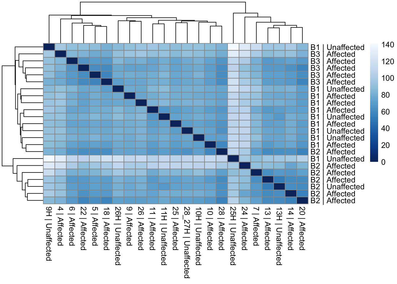
Principal Components Analysis
Our below PCA shows that there does not seem to be a batch-related effect occurring after using limma. However, we can see that our 3 male samples are grouping. Given this knowledge, removing them from downstream analyses is the best option.
pca_data_all <- plotPCA(vsd_limma, intgroup = c("Batch", "Affected", "Sex"),
                        returnData = TRUE)
percent_var_all <- round(100 * attr(pca_data_all, "percentVar"))

ggplot(pca_data_all, aes(PC1, PC2)) +
  geom_point(aes(colour = Affected, fill = Sex, shape = Batch), size = 4) +
  scale_shape_manual(values = c(21, 22, 23)) +
  scale_fill_manual(values = c("white", "gray")) +
  scale_color_manual(values = c("blue", "red")) +
  geom_text(aes(label = name),
    data = subset(pca_data_all, PC2 < -18 | PC1 < -30),
    vjust = -1, hjust = 0.5, size = 2.5
  ) +
  xlab(paste0("PC1: ", percent_var_all[1], "% variance")) +
  ylab(paste0("PC2: ", percent_var_all[2], "% variance")) +
  coord_fixed()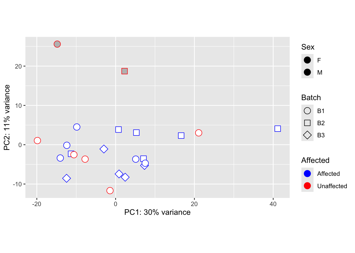
pca_data_all <- plotPCA(vsd_limma, intgroup = c("Affected", "Sex",
                                                "Category"),
                        returnData = TRUE)
percent_var_all <- round(100 * attr(pca_data_all, "percentVar"))

ggplot(pca_data_all, aes(PC1, PC2)) +
  geom_point(aes(colour = Category, fill = Sex, shape = Affected), size = 4) +
  scale_shape_manual(values = c(21, 22, 23)) +
  scale_fill_manual(values = c("white", "gray")) +
  geom_text(aes(label = name), vjust = -1, hjust = 0.65, size = 5) +
  # geom_text_repel(aes(label = name), size = 5, vjust = -1, hjust = -0.65) +
  xlab(paste0("PC1: ", percent_var_all[1], "% variance")) +
  ylab(paste0("PC2: ", percent_var_all[2], "% variance")) +
  coord_fixed()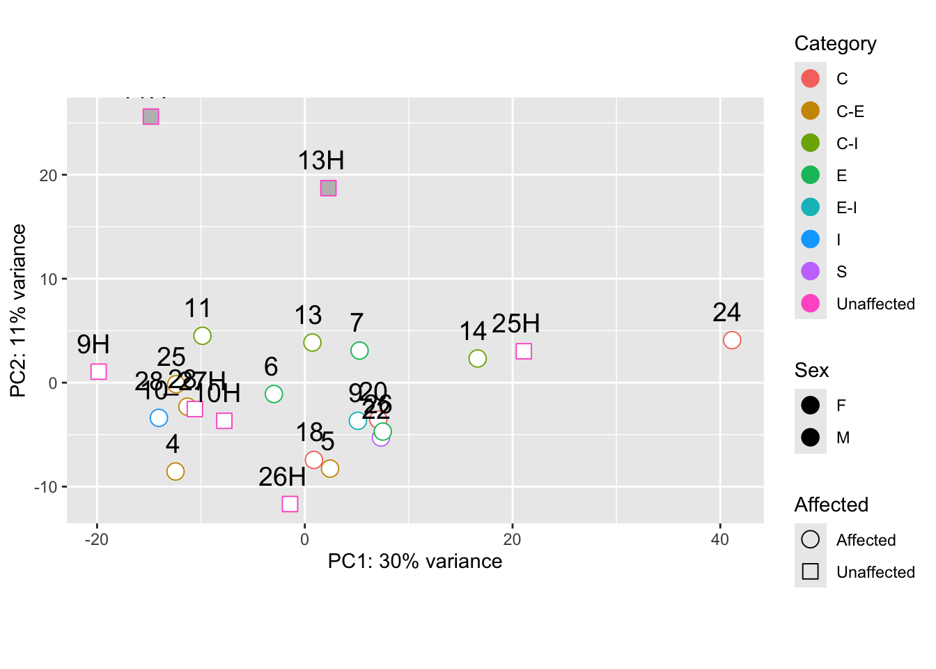
pca_data <- plotPCA(vsd_limma, intgroup = c("Sex", "Affected"), returnData = TRUE)
percent_var <- round(100 * attr(pca_data, "percentVar"))

ggplot(pca_data, aes(PC1, PC2)) +
  geom_point(aes(shape = Sex, colour = Affected), size = 5) +
  scale_color_manual(
    values = c("blue", "red"),
    name = "Affected Status",
    labels = c("Unaffected", "Affected")
  ) +
  scale_shape_manual(
    name = "Sex",
    labels = c("Male", "Female"),
    values = c(16, 17)
  ) + # Example shapes, change as needed
  geom_text_repel(aes(label = name), size = 5, vjust = -2, hjust = -0.65) +
  xlab(paste0("PC1: ", percent_var[1], "% variance")) +
  ylab(paste0("PC2: ", percent_var[2], "% variance")) +
  coord_fixed()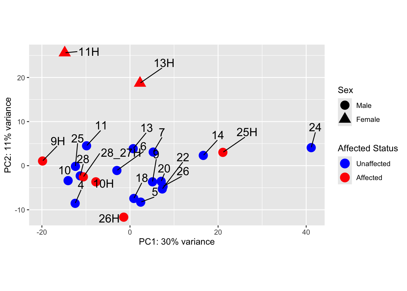
pca_data_all <- plotPCA(vsd_limma, intgroup = c("Category"),
                        returnData = TRUE)
percent_var_all <- round(100 * attr(pca_data_all, "percentVar"))

ggplot(pca_data_all, aes(PC1, PC2)) +
  geom_point(aes(colour = Category), size = 5) +
  scale_colour_manual(
    values = c(
      "#B3DE69", "#FFFFB3", "#BEBADA", "#FB8072", "#80B1D3",
      "#FCCDE5", "#8DD3C7", "#000000"
    ),
    name = "Category"
  ) +
  # geom_text(aes(label = name), vjust = -.75, hjust = -.5, size = 3) +
  # geom_text_repel(aes(label = name), size = 5, vjust = -2, hjust = -0.65) +
  geom_text_repel(aes(label = name), size = 3) +
  xlab(paste0("PC1: ", percent_var_all[1], "% variance")) +
  ylab(paste0("PC2: ", percent_var_all[2], "% variance")) +
  ggthemes::theme_clean()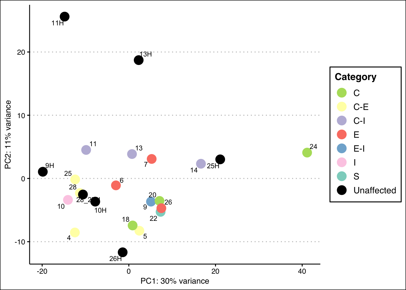
Heatmap of all genes, top 50 & top 100 genes
# Specify annotation colors by columns
# Use RColorBrewer::brewer.pal(n=10, name="Set1")
category_colors <- c(
"Autoimmune disorder" = "#B3DE69",
"Immunodeficiency" = "#FFFFB3",
"Channelopathy" = "#BEBADA",
"Inflammatory disorder" = "#FB8072",
"Metabolic disorder" = "#80B1D3",
"Mitochondrial disorder" = "#FCCDE5",
"Neurologic disorder" = "#D9D9D9",
"Myasthenic disorder" = "#FDB462",
"Neuropathy" = "#8DD3C7",
"Unaffected" = "darkgrey"
)
combined_category_colors <- c(
"E" = "#E41A1C", # Dark green
"C-I" = "#377EB8", # Dark orange
"E-I" = "#4DAF4A", # Light purple
"C" = "#984EA3", # Magenta
"I" = "#FF7F00", # Light green
"C-E" = "#FFFF33", # Mustard yellow
"S" = "#F781BF", # Brown
"Unaffected" = "darkgray" # Dark grey
)
# Specify colors
ann_colors <- list(
Batch = c(B1 = "purple", B2 = "firebrick", B3 = "yellow"),
Affected = c(Affected = "green", Unaffected = "navy"),
SubCategory = category_colors,
Category = combined_category_colors
)
ann_colors2 <- list(
Batch = c(B1 = "purple", B2 = "firebrick", B3 = "yellow"),
Affected = c(Affected = "green", Unaffected = "navy"),
SubCategory = category_colors,
Category = combined_category_colors
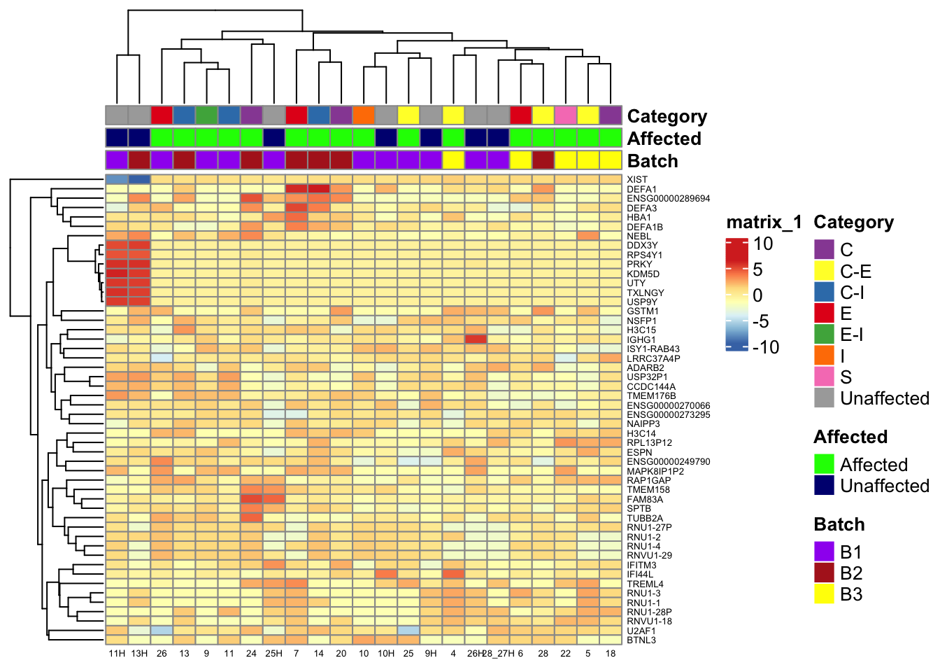
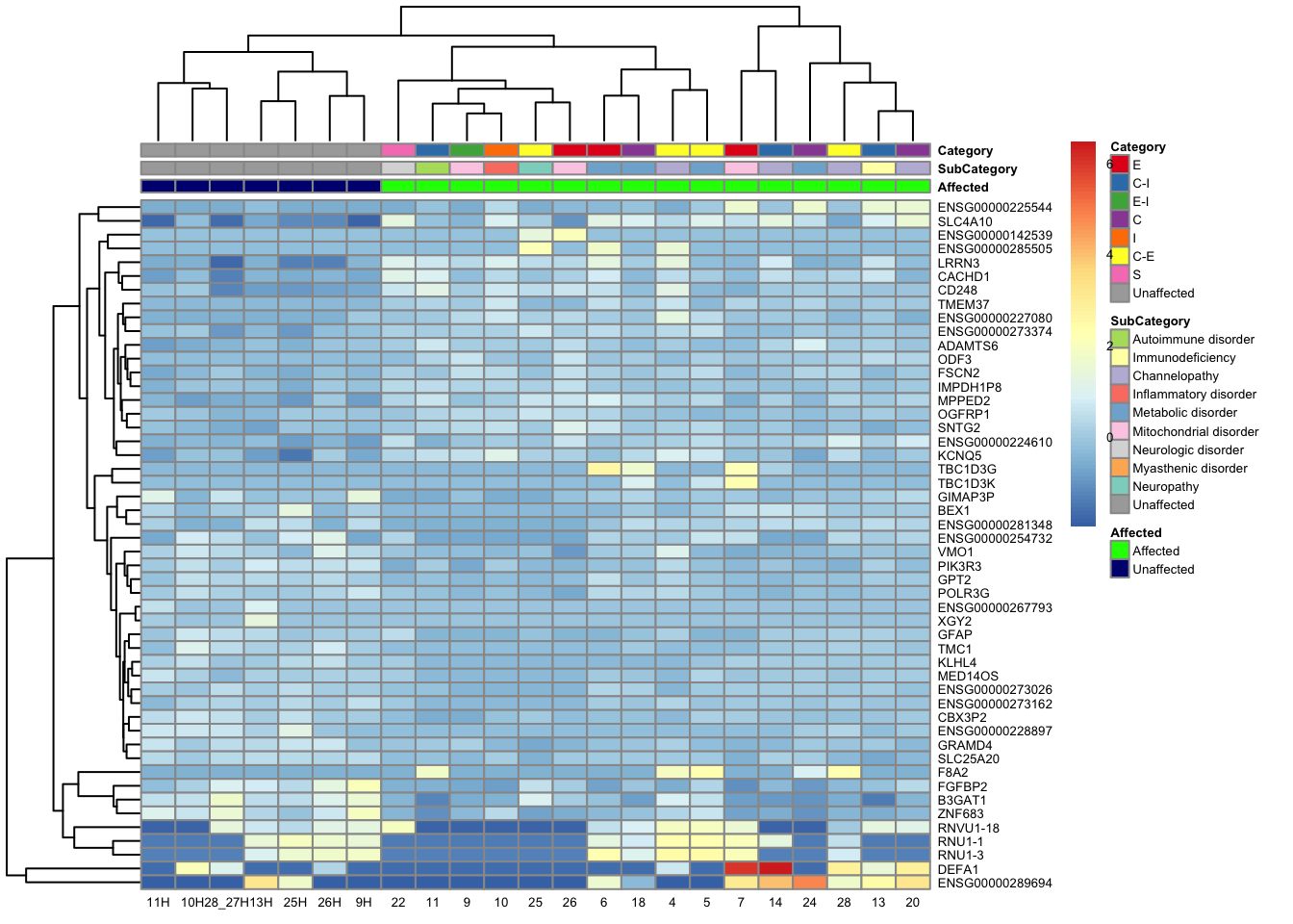
)This is a heatmap of the top 50 genes with the highest variance across samples
top_var_genes <- head(order(-rowVars(assay(vsd_limma))), 50)
mat <- assay(vsd_limma)[top_var_genes, ]
mat <- mat - rowMeans(mat)
df <- as.data.frame(colData(vsd_limma)[, c("Batch", "Affected", "Category")])

ensembl_to_gene <- setNames(gene_info$gene_name, gene_info$Ensembl_ID)

# Get the current row names of the matrix 'mat'
current_ensembl_ids <- rownames(mat)

# Find the corresponding gene names for the Ensembl IDs
new_row_names <- ensembl_to_gene[current_ensembl_ids]

# Set the new row names for the matrix 'mat'
rownames(mat) <- new_row_names

ComplexHeatmap::pheatmap(mat,
  annotation_col = df, annotation_colors = ann_colors2,
  fontsize = 5, angle_col = c("0")
)
This is a heatmap of the top 50 genes with the highest variance across all samples.
top_var_genes_all <- head(order(-rowVars(assay(vsd_limma))), 50)
mat_all <- assay(vsd_limma)[top_var_genes_all, ]
mat_all <- mat_all - rowMeans(mat_all)
df_all <- as.data.frame(colData(vsd_limma)[, c("Batch", "Affected", "SubCategory")])
df_affcat <- as.data.frame(colData(vsd_limma)[, c("Affected", "Category")])

ensembl_to_gene <- setNames(gene_info$gene_name, gene_info$Ensembl_ID)

# Get the current row names of the matrix 'mat'
current_ensembl_ids_all <- rownames(mat_all)

# Find the corresponding gene names for the Ensembl IDs
new_row_names_all <- ensembl_to_gene[current_ensembl_ids_all]

# Set the new row names for the matrix 'mat'
rownames(mat_all) <- new_row_names_all

pheatmap(mat_all, annotation_col = df_all, annotation_colors = ann_colors,
         fontsize = 5)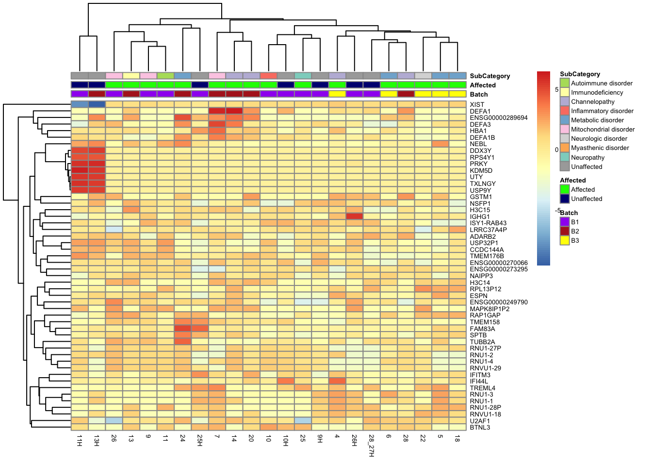
pheatmap(mat_all, annotation_col = df_affcat, annotation_colors = ann_colors2,
         fontsize = 5)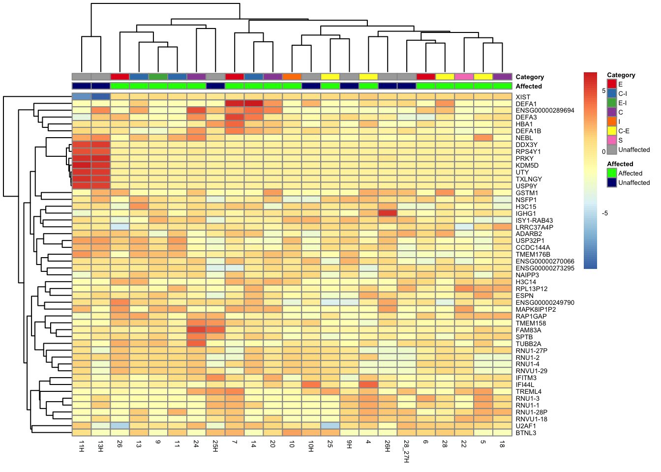
This is a heatmap of the top 100 genes with the highest variance across
top_var_genes_100_all <- head(order(-rowVars(assay(vsd_limma))), 100)
mat_100_all <- assay(vsd_limma)[top_var_genes_100_all, ]
mat_100_all <- mat_100_all - rowMeans(mat_100_all)
df_100_all <- as.data.frame(colData(vsd_limma)[, c("Affected", "SubCategory")])

ensembl_to_gene <- setNames(gene_info$gene_name, gene_info$Ensembl_ID)

# Get the current row names of the matrix 'mat'
current_ensembl_ids_100_all <- rownames(mat_100_all)

# Find the corresponding gene names for the Ensembl IDs
new_row_names_100_all <- ensembl_to_gene[current_ensembl_ids_100_all]

# Set the new row names for the matrix 'mat'
rownames(mat_100_all) <- new_row_names_100_all

pheatmap(mat_100_all, annotation_col = df_100_all,
         annotation_colors = ann_colors2, fontsize = 6)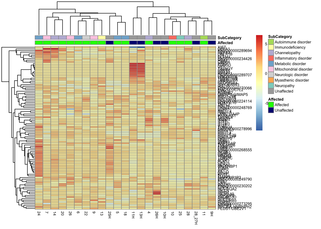
Comparison/Contrast of Affected_Affected_vs_Unaffected
res_aff_vs_unaff_sub <- results(dds, contrast = c("Affected", "Affected", "Unaffected"))
res_aff_vs_unaff_df_sub <- process_and_save_results(
  res_aff_vs_unaff_sub,
  "output/res_aff_vs_unaff_sub.csv"
)
res_aff_vs_unaff_df_sub <- arrange(res_aff_vs_unaff_df_sub, padj)
res_aff_vs_unaff_df_05_sub <- subset(res_aff_vs_unaff_df_sub, padj < 0.05)
res_aff_vs_unaff_df_1_sub <- subset(res_aff_vs_unaff_df_sub, padj < 0.1)

summary(res_aff_vs_unaff_sub)
out of 24628 with nonzero total read count
adjusted p-value < 0.1
LFC > 0 (up)       : 22, 0.089%
LFC < 0 (down)     : 28, 0.11%
outliers [1]       : 164, 0.67%
low counts [2]     : 0, 0%
(mean count < 0)
[1] see 'cooksCutoff' argument of ?results
[2] see 'independentFiltering' argument of ?results
topgenes_byensemblid_sub <- head(rownames(res_aff_vs_unaff_df_sub), 100)
topgenes_aff_vs_unaff_05_sub <- assay(vsd_limma)[topgenes_byensemblid_sub, ]
topgenes_aff_vs_unaff_05_sub <- topgenes_aff_vs_unaff_05_sub - rowMeans(topgenes_aff_vs_unaff_05_sub)
ensembl_to_gene_sub <- setNames(gene_info$gene_name, gene_info$Ensembl_ID)
# Get the current row names of the matrix 'mat'
current_ensembl_ids_sub <- rownames(topgenes_aff_vs_unaff_05_sub)
# Find the corresponding gene names for the Ensembl IDs
new_row_names_sub <- ensembl_to_gene_sub[current_ensembl_ids_sub]
# Set the new row names for the matrix 'mat'
rownames(topgenes_aff_vs_unaff_05_sub) <- new_row_names_sub
topgenes_aff_vs_unaff_05_sub <- topgenes_aff_vs_unaff_05_sub[order(row.names(topgenes_aff_vs_unaff_05_sub)), ]
df_sub <- as.data.frame(colData(vsd_limma)[, c("Affected", "Category")])
pheatmap(topgenes_aff_vs_unaff_05_sub, annotation_col = df_sub, annotation_colors = ann_colors2, fontsize = 5, angle_col = c("0"))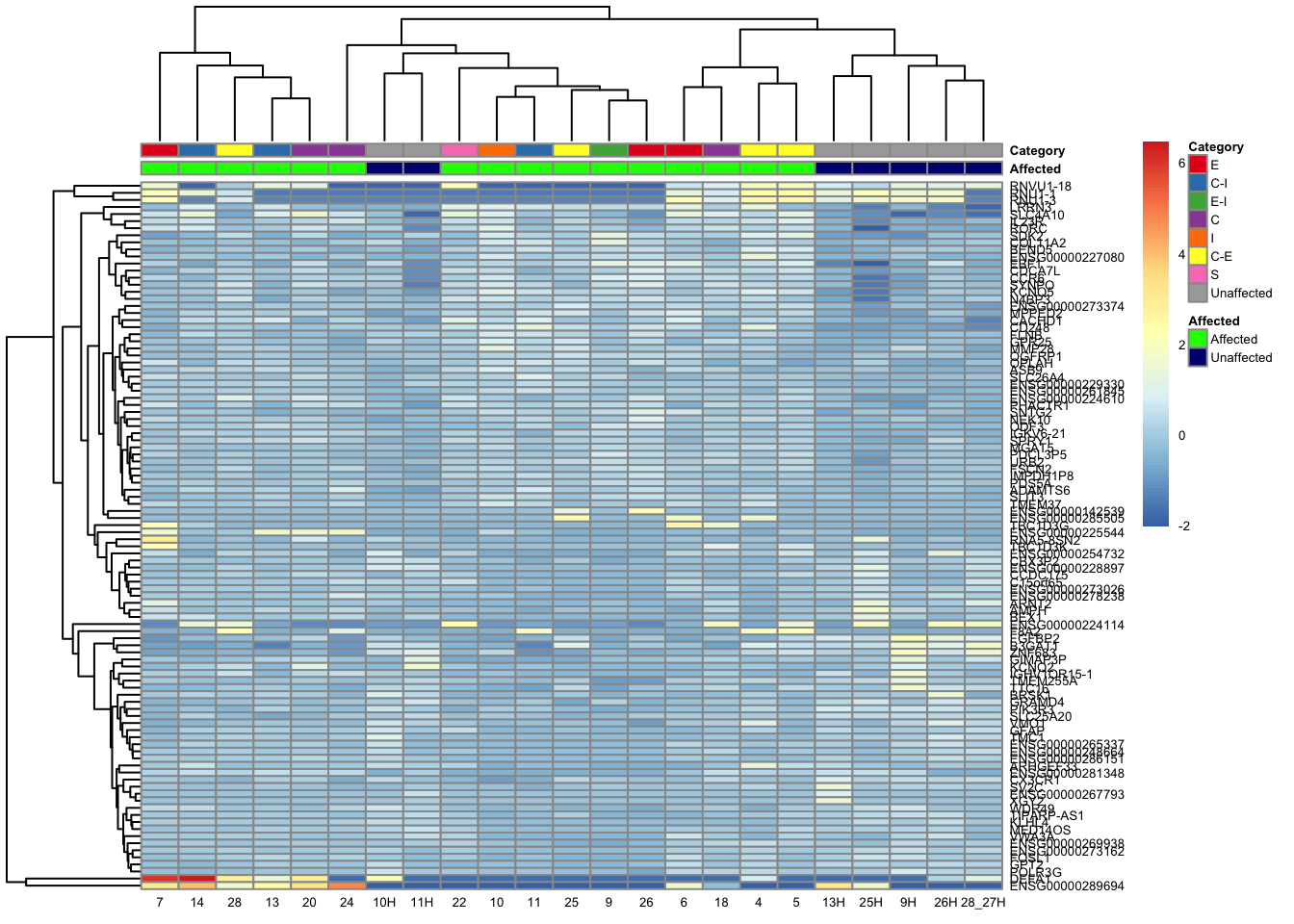
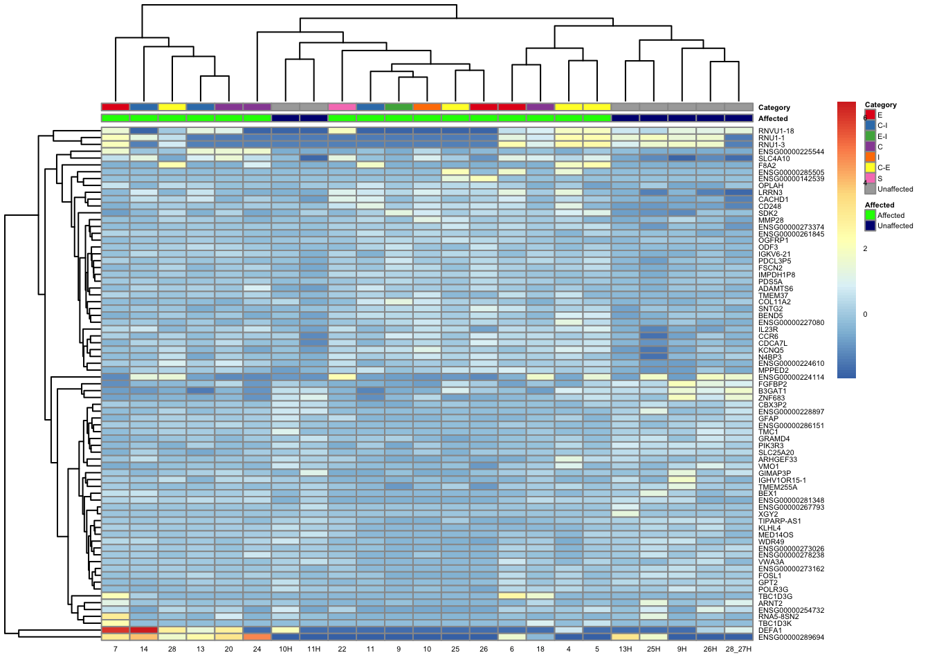
topgenes_byensemblid_sub <- head(rownames(res_aff_vs_unaff_df_sub), 100)
topgenes_aff_vs_unaff_05_sub <- assay(vsd_limma)[topgenes_byensemblid_sub, ]
topgenes_aff_vs_unaff_05_sub <- topgenes_aff_vs_unaff_05_sub - rowMeans(topgenes_aff_vs_unaff_05_sub)

ensembl_to_gene_sub <- setNames(gene_info$gene_name, gene_info$Ensembl_ID)

# Get the current row names of the matrix 'mat'
current_ensembl_ids_sub <- rownames(topgenes_aff_vs_unaff_05_sub)

# Find the corresponding gene names for the Ensembl IDs
new_row_names_sub <- ensembl_to_gene_sub[current_ensembl_ids_sub]

# Set the new row names for the matrix 'mat'
rownames(topgenes_aff_vs_unaff_05_sub) <- new_row_names_sub

topgenes_aff_vs_unaff_05_sub <- topgenes_aff_vs_unaff_05_sub[order(row.names(topgenes_aff_vs_unaff_05_sub)), ]

df_sub <- as.data.frame(colData(vsd_limma)[, c("Affected", "SubCategory", "Category")])
pheatmap(topgenes_aff_vs_unaff_05_sub, annotation_col = df_sub, annotation_colors = ann_colors2, fontsize = 5, angle_col = 0)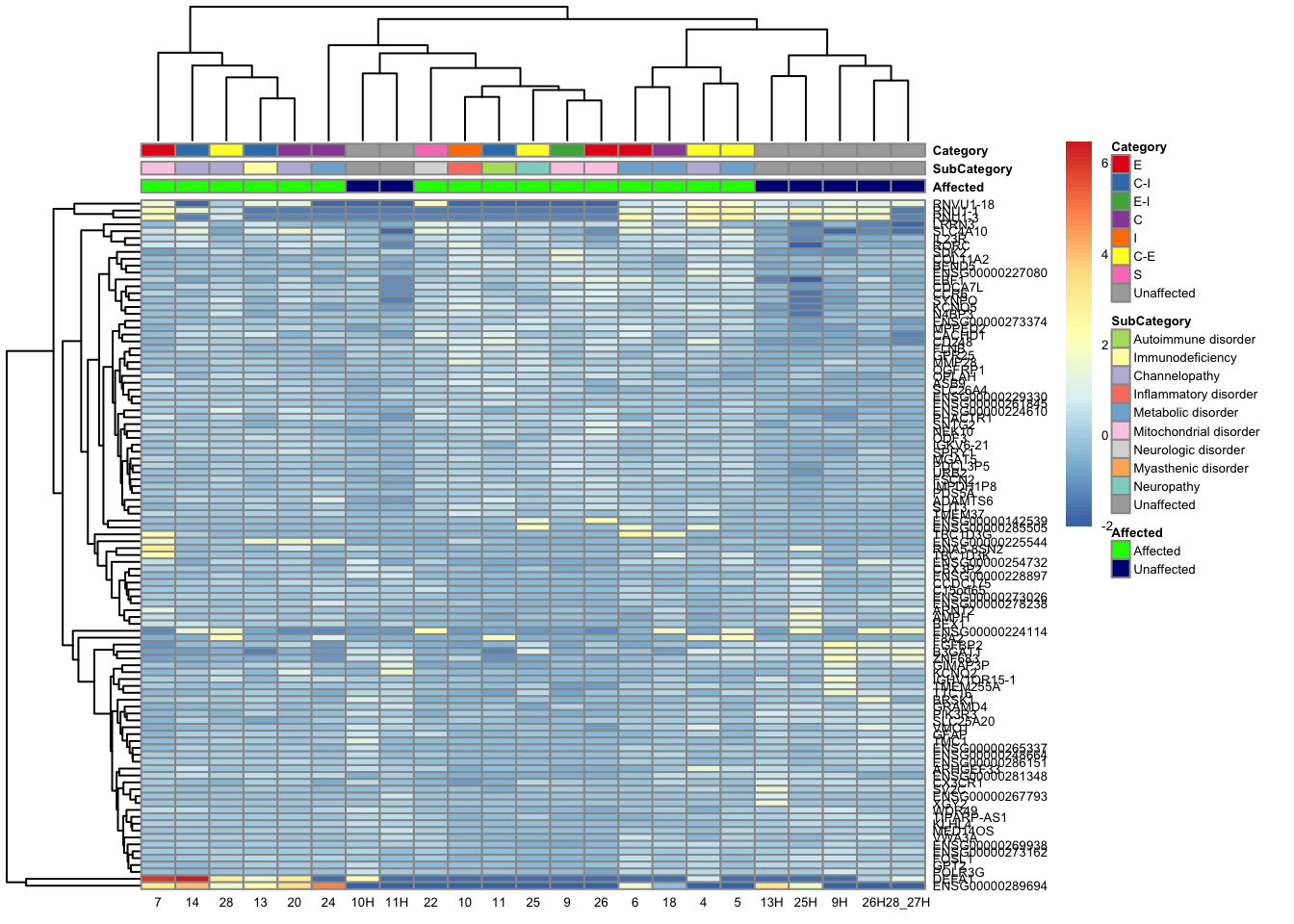
topgenes_byensemblid_sub <- head(rownames(res_aff_vs_unaff_df_sub), 50)
topgenes_aff_vs_unaff_05_sub <- assay(vsd_limma)[topgenes_byensemblid_sub, ]
topgenes_aff_vs_unaff_05_sub <- topgenes_aff_vs_unaff_05_sub - rowMeans(topgenes_aff_vs_unaff_05_sub)

ensembl_to_gene_sub <- setNames(gene_info$gene_name, gene_info$Ensembl_ID)

# Get the current row names of the matrix 'mat'
current_ensembl_ids_sub <- rownames(topgenes_aff_vs_unaff_05_sub)

# Find the corresponding gene names for the Ensembl IDs
new_row_names_sub <- ensembl_to_gene_sub[current_ensembl_ids_sub]

# Set the new row names for the matrix 'mat'
rownames(topgenes_aff_vs_unaff_05_sub) <- new_row_names_sub

topgenes_aff_vs_unaff_05_sub <- topgenes_aff_vs_unaff_05_sub[order(row.names(topgenes_aff_vs_unaff_05_sub)), ]

df_sub <- df <- colData(vsd_limma) %>%
  as.data.frame() %>%
  dplyr::select(Category)
pheatmap(topgenes_aff_vs_unaff_05_sub, annotation_col = df_sub, annotation_colors = ann_colors2, fontsize = 5, angle_col = 0)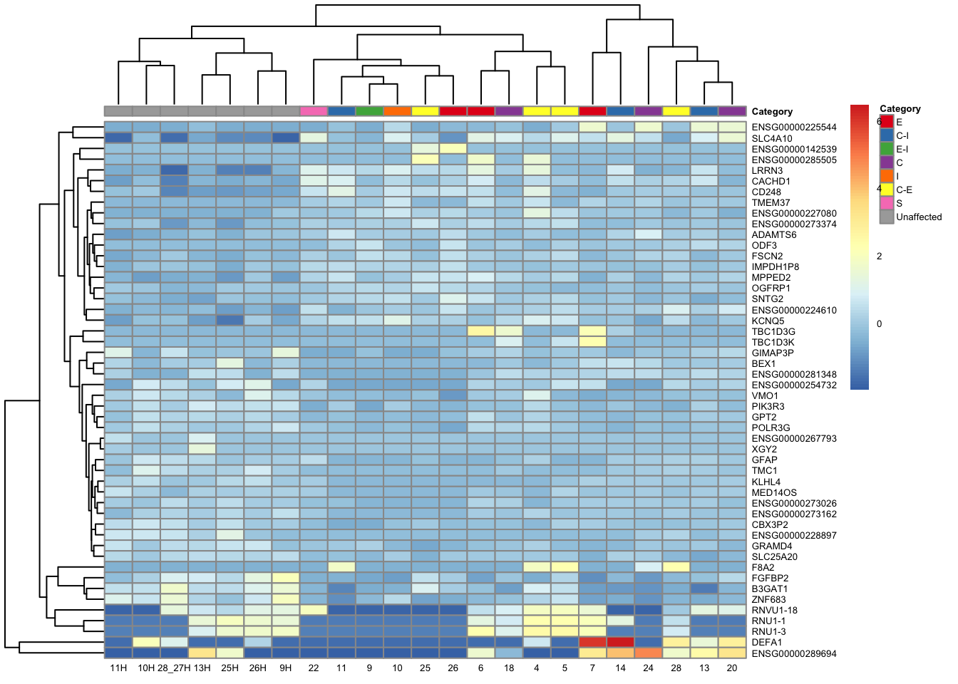
topgenes_byensemblid_sub <- head(rownames(res_aff_vs_unaff_df_sub), 50)
topgenes_aff_vs_unaff_05_sub <- assay(vsd_limma)[topgenes_byensemblid_sub, ]
topgenes_aff_vs_unaff_05_sub <- topgenes_aff_vs_unaff_05_sub - rowMeans(topgenes_aff_vs_unaff_05_sub)

ensembl_to_gene_sub <- setNames(gene_info$gene_name, gene_info$Ensembl_ID)

# Get the current row names of the matrix 'mat'
current_ensembl_ids_sub <- rownames(topgenes_aff_vs_unaff_05_sub)

# Find the corresponding gene names for the Ensembl IDs
new_row_names_sub <- ensembl_to_gene_sub[current_ensembl_ids_sub]

# Set the new row names for the matrix 'mat'
rownames(topgenes_aff_vs_unaff_05_sub) <- new_row_names_sub

topgenes_aff_vs_unaff_05_sub <- topgenes_aff_vs_unaff_05_sub[order(row.names(topgenes_aff_vs_unaff_05_sub)), ]

df_sub <- df <- colData(vsd_limma) %>%
  as.data.frame() %>%
  dplyr::select(Affected, SubCategory, Category)
pheatmap(topgenes_aff_vs_unaff_05_sub,
  annotation_col = df_sub,
  annotation_colors = ann_colors2, fontsize = 5, angle_col = 0
)
Heatmap of Significant Genes
# Assuming 'res_aff_vs_unaff_df_sub' has a column 'padj' for adjusted p-values or 'pvalue' for p-values
# Ensure the row names of 'res_aff_vs_unaff_df_sub' are Ensembl IDs
res_aff_vs_unaff_df_sub <- res_aff_vs_unaff_df_sub[order(res_aff_vs_unaff_df_sub$padj), ]

# Get the top 50 most significant genes based on adjusted p-values
topgenes_byensemblid_sub <- head(rownames(res_aff_vs_unaff_df_sub), 50)

# Extract the corresponding subset of the data matrix
topgenes_aff_vs_unaff_05_sub <- assay(vsd_limma)[topgenes_byensemblid_sub, ]

# Normalize by subtracting the row means
topgenes_aff_vs_unaff_05_sub <- topgenes_aff_vs_unaff_05_sub - rowMeans(topgenes_aff_vs_unaff_05_sub)

# Map Ensembl IDs to gene names
ensembl_to_gene_sub <- setNames(gene_info$gene_name, gene_info$Ensembl_ID)
current_ensembl_ids_sub <- rownames(topgenes_aff_vs_unaff_05_sub)
new_row_names_sub <- ensembl_to_gene_sub[current_ensembl_ids_sub]
rownames(topgenes_aff_vs_unaff_05_sub) <- new_row_names_sub

# Order the matrix based on significance (most significant to least significant)
topgenes_aff_vs_unaff_05_sub <- topgenes_aff_vs_unaff_05_sub[order(res_aff_vs_unaff_df_sub$padj[topgenes_byensemblid_sub]), ]

df_sub <- df <- colData(vsd_limma) %>%
  as.data.frame() %>%
  dplyr::select(Category)

ComplexHeatmap::pheatmap(topgenes_aff_vs_unaff_05_sub, color = colorRampPalette(rev(brewer.pal(n = 9, name =
  "RdYlBu")))(50), annotation_col = df_sub, annotation_colors = ann_colors2, fontsize = 6, angle_col = c("0"), cellheight = 10, cellwidth = 24, border_color = "black", heatmap_legend_param = list(
        title = ""
    ))
topgenes_byensemblid_sub <- head(rownames(res_aff_vs_unaff_df_sub), 50)
topgenes_aff_vs_unaff_05_sub <- assay(vsd_limma)[topgenes_byensemblid_sub, ]
topgenes_aff_vs_unaff_05_sub <- topgenes_aff_vs_unaff_05_sub - rowMeans(topgenes_aff_vs_unaff_05_sub)

ensembl_to_gene_sub <- setNames(gene_info$gene_name, gene_info$Ensembl_ID)

# Get the current row names of the matrix 'mat'
current_ensembl_ids_sub <- rownames(topgenes_aff_vs_unaff_05_sub)

# Find the corresponding gene names for the Ensembl IDs
new_row_names_sub <- ensembl_to_gene_sub[current_ensembl_ids_sub]

# Set the new row names for the matrix 'mat'
rownames(topgenes_aff_vs_unaff_05_sub) <- new_row_names_sub

topgenes_aff_vs_unaff_05_sub <- topgenes_aff_vs_unaff_05_sub[order(row.names(topgenes_aff_vs_unaff_05_sub)), ]

df_sub <- df <- colData(vsd_limma) %>%
  as.data.frame() %>%
  dplyr::select(Affected, SubCategory, Category)
pheatmap(topgenes_aff_vs_unaff_05_sub, annotation_col = df_sub, annotation_colors = ann_colors2, fontsize = 5, angle_col = 0)
topgenes_byensemblid_sub <- head(rownames(res_aff_vs_unaff_df_sub), 75)
topgenes_aff_vs_unaff_05_sub <- assay(vsd_limma)[topgenes_byensemblid_sub, ]
topgenes_aff_vs_unaff_05_sub <- topgenes_aff_vs_unaff_05_sub - rowMeans(topgenes_aff_vs_unaff_05_sub)

ensembl_to_gene_sub <- setNames(gene_info$gene_name, gene_info$Ensembl_ID)

# Get the current row names of the matrix 'mat'
current_ensembl_ids_sub <- rownames(topgenes_aff_vs_unaff_05_sub)

# Find the corresponding gene names for the Ensembl IDs
new_row_names_sub <- ensembl_to_gene_sub[current_ensembl_ids_sub]

# Set the new row names for the matrix 'mat'
rownames(topgenes_aff_vs_unaff_05_sub) <- new_row_names_sub

topgenes_aff_vs_unaff_05_sub <- topgenes_aff_vs_unaff_05_sub[order(row.names(topgenes_aff_vs_unaff_05_sub)), ]

df_sub <- as.data.frame(colData(vsd_limma)[, c("Affected", "Category")])
pheatmap(topgenes_aff_vs_unaff_05_sub,
  annotation_col = df_sub,
  annotation_colors = ann_colors2, fontsize = 4, angle_col = 0
)
topgenes_byensemblid_sub <- head(rownames(res_aff_vs_unaff_df_sub), 75)
topgenes_aff_vs_unaff_05_sub <- assay(vsd_limma)[topgenes_byensemblid_sub, ]
topgenes_aff_vs_unaff_05_sub <- topgenes_aff_vs_unaff_05_sub - rowMeans(topgenes_aff_vs_unaff_05_sub)

ensembl_to_gene_sub <- setNames(gene_info$gene_name, gene_info$Ensembl_ID)

# Get the current row names of the matrix 'mat'
current_ensembl_ids_sub <- rownames(topgenes_aff_vs_unaff_05_sub)

# Find the corresponding gene names for the Ensembl IDs
new_row_names_sub <- ensembl_to_gene_sub[current_ensembl_ids_sub]

# Set the new row names for the matrix 'mat'
rownames(topgenes_aff_vs_unaff_05_sub) <- new_row_names_sub

topgenes_aff_vs_unaff_05_sub <- topgenes_aff_vs_unaff_05_sub[order(row.names(topgenes_aff_vs_unaff_05_sub)), ]

df_sub <- as.data.frame(colData(vsd_limma)[, c("Affected", "SubCategory", "Category")])
pheatmap(topgenes_aff_vs_unaff_05_sub, annotation_col = df_sub, annotation_colors = ann_colors2, fontsize = 4, angle_col = 0)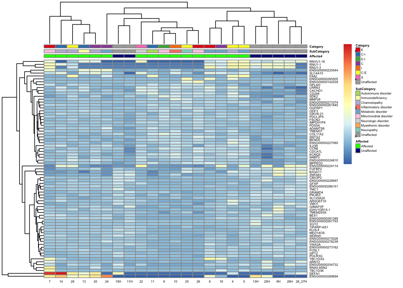
topgenes_byensemblid_sub <- head(rownames(res_aff_vs_unaff_df_sub), 200)
topgenes_aff_vs_unaff_05_sub <- assay(vsd_limma)[topgenes_byensemblid_sub, ]
topgenes_aff_vs_unaff_05_sub <- topgenes_aff_vs_unaff_05_sub - rowMeans(topgenes_aff_vs_unaff_05_sub)

ensembl_to_gene_sub <- setNames(gene_info$gene_name, gene_info$Ensembl_ID)

# Get the current row names of the matrix 'mat'
current_ensembl_ids_sub <- rownames(topgenes_aff_vs_unaff_05_sub)

# Find the corresponding gene names for the Ensembl IDs
new_row_names_sub <- ensembl_to_gene_sub[current_ensembl_ids_sub]

# Set the new row names for the matrix 'mat'
rownames(topgenes_aff_vs_unaff_05_sub) <- new_row_names_sub

topgenes_aff_vs_unaff_05_sub <- topgenes_aff_vs_unaff_05_sub[order(row.names(topgenes_aff_vs_unaff_05_sub)), ]

df_sub <- as.data.frame(colData(vsd_limma)[, c("Affected", "Category")])
pheatmap(topgenes_aff_vs_unaff_05_sub, annotation_col = df_sub, annotation_colors = ann_colors2, fontsize = 4, angle_col = 0)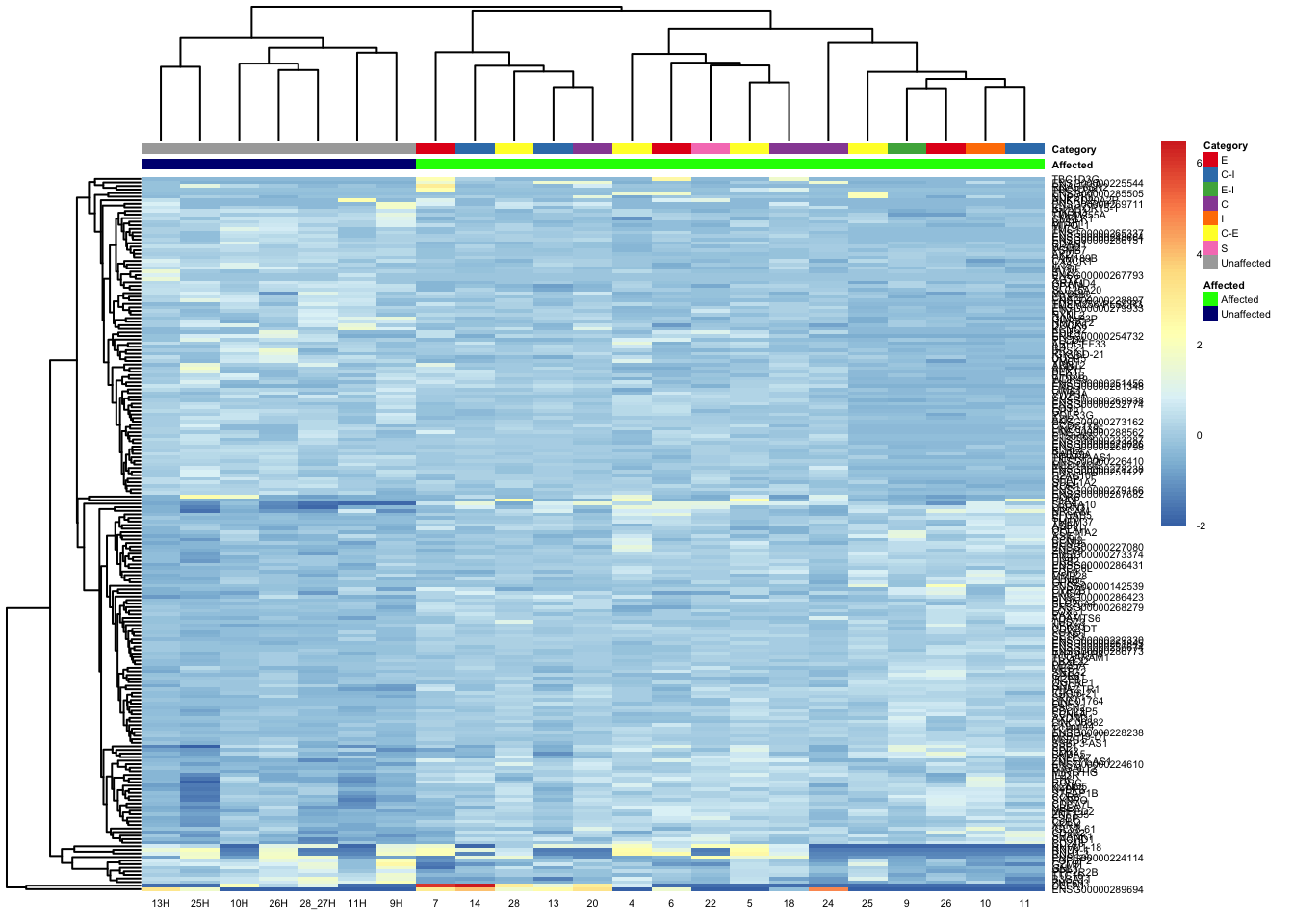
topgenes_byensemblid_sub <- head(rownames(res_aff_vs_unaff_df_sub), 200)
topgenes_aff_vs_unaff_05_sub <- assay(vsd_limma)[topgenes_byensemblid_sub, ]
topgenes_aff_vs_unaff_05_sub <- topgenes_aff_vs_unaff_05_sub - rowMeans(topgenes_aff_vs_unaff_05_sub)

ensembl_to_gene_sub <- setNames(gene_info$gene_name, gene_info$Ensembl_ID)

# Get the current row names of the matrix 'mat'
current_ensembl_ids_sub <- rownames(topgenes_aff_vs_unaff_05_sub)

# Find the corresponding gene names for the Ensembl IDs
new_row_names_sub <- ensembl_to_gene_sub[current_ensembl_ids_sub]

# Set the new row names for the matrix 'mat'
rownames(topgenes_aff_vs_unaff_05_sub) <- new_row_names_sub

topgenes_aff_vs_unaff_05_sub <- topgenes_aff_vs_unaff_05_sub[order(row.names(topgenes_aff_vs_unaff_05_sub)), ]

df_sub <- as.data.frame(colData(vsd_limma)[, c("Affected", "SubCategory", "Category")])
pheatmap(topgenes_aff_vs_unaff_05_sub, annotation_col = df_sub, annotation_colors = ann_colors2, fontsize = 2.25, angle_col = 0)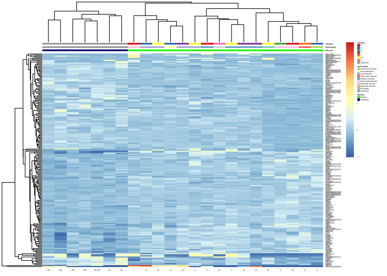
topgenes_byensemblid_sub <- head(rownames(res_aff_vs_unaff_df_sub), 125)
topgenes_aff_vs_unaff_05_sub <- assay(vsd_limma)[topgenes_byensemblid_sub, ]
topgenes_aff_vs_unaff_05_sub <- topgenes_aff_vs_unaff_05_sub - rowMeans(topgenes_aff_vs_unaff_05_sub)

ensembl_to_gene_sub <- setNames(gene_info$gene_name, gene_info$Ensembl_ID)

# Get the current row names of the matrix 'mat'
current_ensembl_ids_sub <- rownames(topgenes_aff_vs_unaff_05_sub)

# Find the corresponding gene names for the Ensembl IDs
new_row_names_sub <- ensembl_to_gene_sub[current_ensembl_ids_sub]

# Set the new row names for the matrix 'mat'
rownames(topgenes_aff_vs_unaff_05_sub) <- new_row_names_sub

# topgenes_aff_vs_unaff_05_sub <- topgenes_aff_vs_unaff_05_sub[order(row.names(topgenes_aff_vs_unaff_05_sub)), ]

df_sub <- as.data.frame(colData(vsd_limma)[, c("Affected", "Category")])
pheatmap(topgenes_aff_vs_unaff_05_sub, annotation_col = df_sub, annotation_colors = ann_colors2, fontsize = 3.75, angle_col = 0)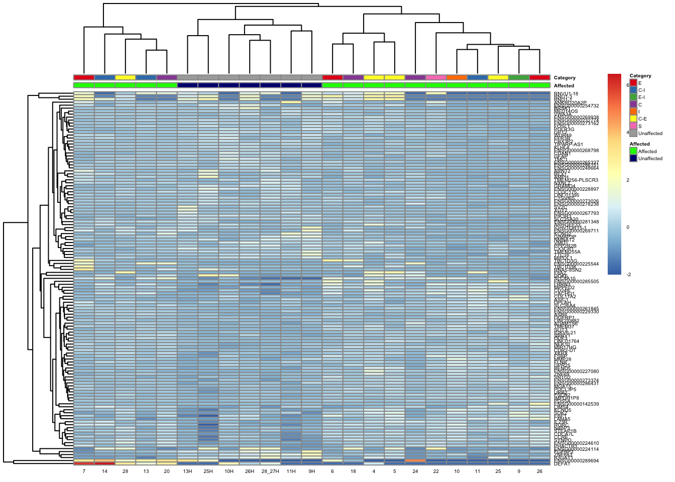
topgenes_byensemblid_sub <- head(rownames(res_aff_vs_unaff_df_sub), 125)
topgenes_aff_vs_unaff_05_sub <- assay(vsd_limma)[topgenes_byensemblid_sub, ]
topgenes_aff_vs_unaff_05_sub <- topgenes_aff_vs_unaff_05_sub - rowMeans(topgenes_aff_vs_unaff_05_sub)

ensembl_to_gene_sub <- setNames(gene_info$gene_name, gene_info$Ensembl_ID)

# Get the current row names of the matrix 'mat'
current_ensembl_ids_sub <- rownames(topgenes_aff_vs_unaff_05_sub)

# Find the corresponding gene names for the Ensembl IDs
new_row_names_sub <- ensembl_to_gene_sub[current_ensembl_ids_sub]

# Set the new row names for the matrix 'mat'
rownames(topgenes_aff_vs_unaff_05_sub) <- new_row_names_sub

# topgenes_aff_vs_unaff_05_sub <- topgenes_aff_vs_unaff_05_sub[order(row.names(topgenes_aff_vs_unaff_05_sub)), ]

df_sub <- as.data.frame(colData(vsd_limma)[, c("Affected", "SubCategory", "Category")])
pheatmap(topgenes_aff_vs_unaff_05_sub, annotation_col = df_sub, annotation_colors = ann_colors2, fontsize = 3.75, angle_col = 0)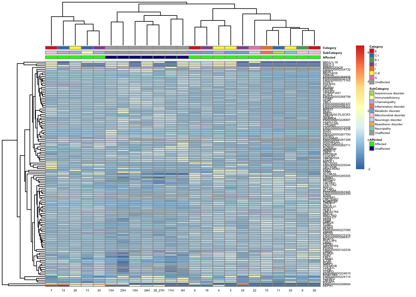
topgenes_byensemblid_sub <- head(rownames(res_aff_vs_unaff_df_sub), 150)
topgenes_aff_vs_unaff_05_sub <- assay(vsd_limma)[topgenes_byensemblid_sub, ]
topgenes_aff_vs_unaff_05_sub <- topgenes_aff_vs_unaff_05_sub - rowMeans(topgenes_aff_vs_unaff_05_sub)

ensembl_to_gene_sub <- setNames(gene_info$gene_name, gene_info$Ensembl_ID)

# Get the current row names of the matrix 'mat'
current_ensembl_ids_sub <- rownames(topgenes_aff_vs_unaff_05_sub)

# Find the corresponding gene names for the Ensembl IDs
new_row_names_sub <- ensembl_to_gene_sub[current_ensembl_ids_sub]

# Set the new row names for the matrix 'mat'
rownames(topgenes_aff_vs_unaff_05_sub) <- new_row_names_sub

# topgenes_aff_vs_unaff_05_sub <- topgenes_aff_vs_unaff_05_sub[order(row.names(topgenes_aff_vs_unaff_05_sub)), ]

df_sub <- as.data.frame(colData(vsd_limma)[, c("Affected", "Category")])
pheatmap(topgenes_aff_vs_unaff_05_sub, annotation_col = df_sub, annotation_colors = ann_colors2, fontsize = 3.5, angle_col = 0)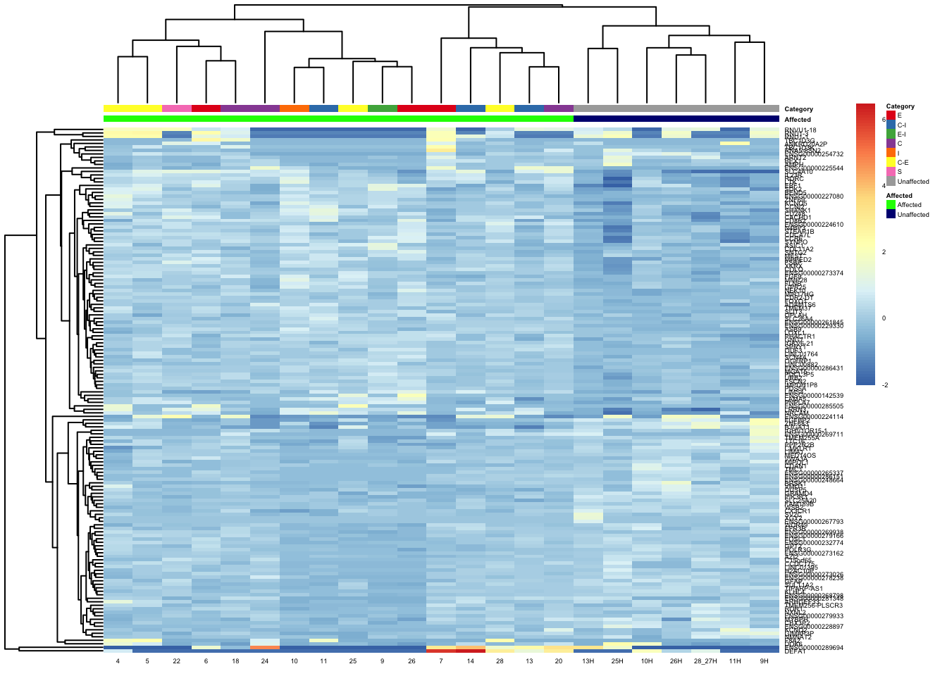
topgenes_byensemblid_sub <- head(rownames(res_aff_vs_unaff_df_sub), 150)
topgenes_aff_vs_unaff_05_sub <- assay(vsd_limma)[topgenes_byensemblid_sub, ]
topgenes_aff_vs_unaff_05_sub <- topgenes_aff_vs_unaff_05_sub - rowMeans(topgenes_aff_vs_unaff_05_sub)

ensembl_to_gene_sub <- setNames(gene_info$gene_name, gene_info$Ensembl_ID)

# Get the current row names of the matrix 'mat'
current_ensembl_ids_sub <- rownames(topgenes_aff_vs_unaff_05_sub)

# Find the corresponding gene names for the Ensembl IDs
new_row_names_sub <- ensembl_to_gene_sub[current_ensembl_ids_sub]

# Set the new row names for the matrix 'mat'
rownames(topgenes_aff_vs_unaff_05_sub) <- new_row_names_sub

# topgenes_aff_vs_unaff_05_sub <- topgenes_aff_vs_unaff_05_sub[order(row.names(topgenes_aff_vs_unaff_05_sub)), ]

df_sub <- as.data.frame(colData(vsd_limma)[, c("Affected", "SubCategory", "Category")])
pheatmap(topgenes_aff_vs_unaff_05_sub, annotation_col = df_sub, annotation_colors = ann_colors2, fontsize = 3.5, angle_col = 0)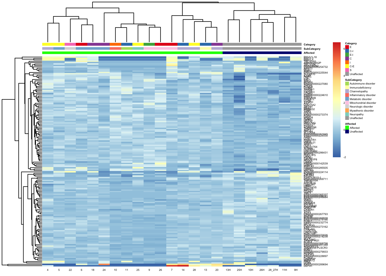
gb_df <- genes_biomart[, c(1, ncol(genes_biomart))]
res_aff_vs_unaff_df_sub_genename <- res_aff_vs_unaff_df_sub
res_aff_vs_unaff_df_sub_genename$Ensembl_ID <- row.names(res_aff_vs_unaff_df_sub)
res_aff_vs_unaff_df_sub_genename <- merge(x = res_aff_vs_unaff_df_sub_genename, y = gene_info, by.x = "Ensembl_ID", by.y = "Ensembl_ID", all.x = TRUE)
res_aff_vs_unaff_df_sub_genename <- res_aff_vs_unaff_df_sub_genename[, c(dim(res_aff_vs_unaff_df_sub_genename)[2], 1:dim(res_aff_vs_unaff_df_sub_genename)[2] - 1)]
res_aff_vs_unaff_df_sub_genename <- res_aff_vs_unaff_df_sub_genename[order(res_aff_vs_unaff_df_sub_genename[, "padj"]), ]
write.csv(res_aff_vs_unaff_df_sub_genename, file = "output/res_aff_vs_unaff_df_sub_genename.csv")
res_aff_vs_unaff_df_genename_05 <- subset(res_aff_vs_unaff_df_sub_genename, padj < 0.05)
res_aff_vs_unaff_df_genename_05 <- res_aff_vs_unaff_df_genename_05[order(res_aff_vs_unaff_df_genename_05$padj), ]
write.csv(res_aff_vs_unaff_df_genename_05, file = "output/res_aff_vs_unaff_df_sub_genename_05.csv")
res_aff_vs_unaff_df_genename_1 <- subset(res_aff_vs_unaff_df_sub_genename, padj < 0.1)
res_aff_vs_unaff_df_genename_1 <- res_aff_vs_unaff_df_genename_1[order(res_aff_vs_unaff_df_genename_1$padj), ]
write.csv(res_aff_vs_unaff_df_genename_1, file = "output/res_aff_vs_unaff_df_sub_genename_padj1.csv")Below is a table of information about the top genes.
genes <- res_aff_vs_unaff_df_genename_05$gene_name
my_gene_data <- queryMany(genes, scopes = "symbol", fields = c("symbol", "name", "summary", species = "human"))
Finished
Pass returnall=TRUE to return lists of duplicate or missing query terms.my_gene_data_unique <- as.data.frame(my_gene_data) %>% dplyr::distinct(query, .keep_all = TRUE)
# paged_table(my_gene_data, options = list(rows.print = 15))filtered_gene_names <- res_aff_vs_unaff_df_sub_genename$gene_name[!grepl("^ENS", res_aff_vs_unaff_df_sub_genename$gene_name)]
# Select specific genes to show
# set top = 0, then specify genes using label.select argument
maplot <- ggmaplot(res_aff_vs_unaff_df_sub,
main = "Affected vs Unaffected MA Plot",
fdr = .1, fc = 1, size = 0.4, # Same used for others.
genenames = as.vector(res_aff_vs_unaff_df_sub_genename$gene_name),
ggtheme = ggplot2::theme_minimal(),
legend = "top", top = 30,
label.select = c("KCNQ5"),
font.label = c("bold", 6), label.rectangle = TRUE,
font.legend = "bold", font.main = "bold"
)
maplot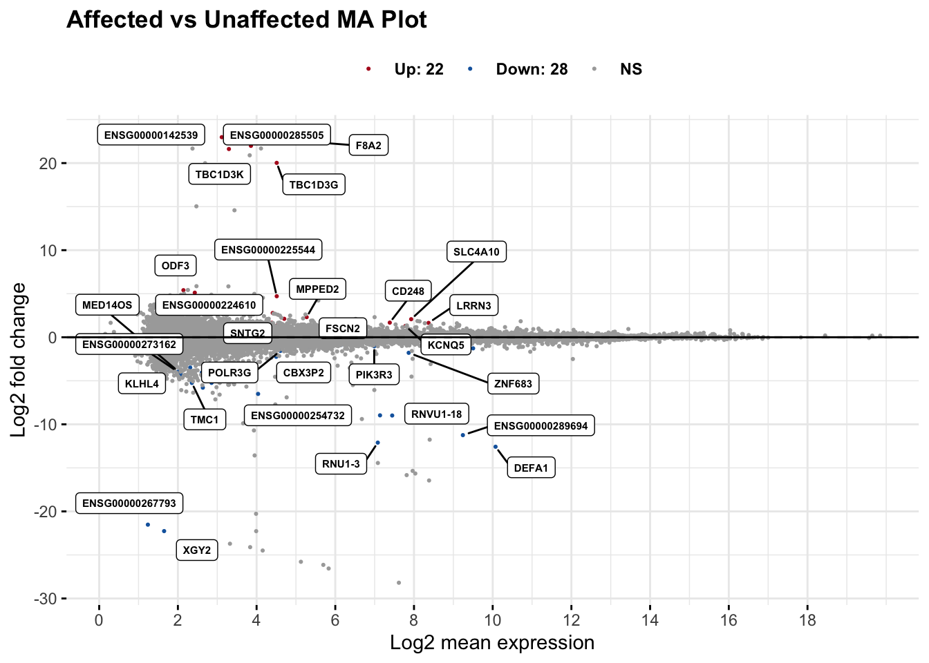
significant_data <- maplot$data %>%
  filter(grepl("Up|Down", sig)) %>%
  mutate(direction = ifelse(grepl("Up", sig), "Up", "Down")) %>%
  dplyr::select(-sig) # This removes the 'sig' column

# Combine DataFrames based on matching 'query' in my_gene_data_unique to 'gene' in significant_data
combined_data <- inner_join(my_gene_data_unique, significant_data, by = c("query" = "name"))

combined_data <- combined_data %>%
  dplyr::select(-notfound, -X_id, -X_score) %>%
  rename(gene = query)

paged_table(as.data.frame(significant_data), options = list(rows.print = 30))
# Save significant genes
write.csv(significant_data, file = "output/res_aff_vs_unaff_significant_subsetted_samples.csv", row.names = FALSE)
# Save significant genes
write.csv(combined_data, file = "output/res_aff_vs_unaff_significant_subsetted_mygene.csv", row.names = FALSE)Expression of Candidate Genes
Below is a table of expression of the genes identified during our WGS analysis.
# Subset gene_info using genes of interest
subset_gene_info <- gene_info[gene_info$gene_name %in% genes_of_interest, ]

filtered_by_interest <- filter(res_aff_vs_unaff_df_sub_genename, Ensembl_ID %in% subset_gene_info$Ensembl_ID)

# Filtering the dataframe by row names
filtered_counts <- counts[row.names(counts) %in% subset_gene_info$Ensembl_ID, ]

# Match and update row names
matching_indices <- match(rownames(filtered_counts), subset_gene_info$Ensembl_ID)

# Update row names based on matching_column values from metadata
rownames(filtered_counts) <- subset_gene_info$gene_name[matching_indices]

missing_genes <- setdiff(subset_gene_info$Ensembl_ID, filtered_by_interest$Ensembl_ID)

corresponding_gene_names <- subset_gene_info$gene_name[subset_gene_info$Ensembl_ID %in% missing_genes]

missing_gene_counts <- counts[row.names(counts) %in% missing_genes, ]

paged_table(filtered_by_interest, options = list(rows.print = 15))
paged_table(filtered_counts, options = list(rows.print = 15))Below is a heatmap highlighting the expression of our genes of interest across batch, disease group, and affected status.
mat3 <- assay(vsd_limma)[filtered_by_interest$Ensembl_ID, ]
rownames(mat3) <- gene_info$gene_name[match(filtered_by_interest$Ensembl_ID, gene_info$Ensembl_ID)]
df_sub <- as.data.frame(colData(vsd_limma)[, c("Affected", "Category")])
pheatmap(mat3, annotation_col = df_sub, annotation_colors = ann_colors2, fontsize = 4, angle_col = 0)
Enrichment analysis
# res <- gost(query = significant_data$name, organism = "hsapiens", significant = FALSE) # should significant be true or false?
#
# x <- gostplot(res, capped = FALSE, interactive = FALSE)
# x + geom_label_repel(aes(label = "term_id"),
#   box.padding   = 0.35,
#   point.padding = 0.5,
#   segment.color = "grey50"
# )
# Your existing code for obtaining geneList with Ensembl IDs
rownames(res_aff_vs_unaff_df_sub) <- gsub("\\..*", "", rownames(res_aff_vs_unaff_df_sub))
res_aff_vs_unaff_df_sub <- res_aff_vs_unaff_df_sub %>% dplyr::distinct()
geneList <- res_aff_vs_unaff_df_sub$log2FoldChange
geneList2 <- res_aff_vs_unaff_df_sub$padj
geneList3 <- res_aff_vs_unaff_df_sub$padj
names(geneList3) <- rownames(res_aff_vs_unaff_df_sub)
names(geneList2) <- rownames(res_aff_vs_unaff_df_sub)
names(geneList) <- rownames(res_aff_vs_unaff_df_sub)
# Initialize BioMart
ensembl <- useMart("ensembl", dataset = "hsapiens_gene_ensembl")
# Convert all Ensembl IDs in geneList to Entrez IDs
attributes <- c("ensembl_gene_id", "entrezgene_id")
filters <- "ensembl_gene_id"
results <- getBM(attributes = attributes, filters = filters, values = names(geneList), mart = ensembl)
results3 <- getBM(attributes = attributes, filters = filters, values = names(geneList2), mart = ensembl)
# Convert all Ensembl IDs in geneList to Entrez IDs
# This is for genes of interest
attributes2 <- c("hgnc_symbol", "ensembl_gene_id", "entrezgene_id")
filters2 <- "hgnc_symbol"
results2 <- getBM(attributes = attributes2, filters = filters2, values = genes_of_interest, mart = ensembl)
# Remove rows with NA or empty Entrez IDs
results <- results[!is.na(results$entrezgene_id) & results$entrezgene_id != "", ]
results3 <- results3[!is.na(results3$entrezgene_id) & results3$entrezgene_id != "", ]
results2 <- results2[!is.na(results2$entrezgene_id) & results2$entrezgene_id != "", ]
# Create a new geneList with Entrez IDs
geneList_entrez <- geneList[results$ensembl_gene_id]
names(geneList_entrez) <- results$entrezgene_id
# Create a new geneList with Entrez IDs
geneList_entrez2 <- geneList2[results3$ensembl_gene_id]
names(geneList_entrez2) <- results3$entrezgene_id
# Create a new geneList with Entrez IDs
geneList_entrez3 <- geneList3[results2$ensembl_gene_id]
names(geneList_entrez3) <- results2$entrezgene_id
# Filter genes with abs(log2FoldChange) > 2
gene_entrez <- names(geneList_entrez)[abs(geneList_entrez) > 2]
# Filter genes with padj < .05
gene_entrez2 <- names(geneList_entrez2)[!is.na(geneList_entrez2) & geneList_entrez2 < .05]
# Run enrichGO with Entrez IDs
ego_cc <- enrichGO(
gene = gene_entrez,
universe = names(geneList_entrez),
OrgDb = org.Hs.eg.db,
ont = "CC",
pAdjustMethod = "BH",
pvalueCutoff = 0.01,
qvalueCutoff = 0.05,
readable = TRUE
)
# Plot results
dotplot(ego_cc, showCategory = 10, title = "Overrepresented Cellular Components") + ggthemes::theme_clean()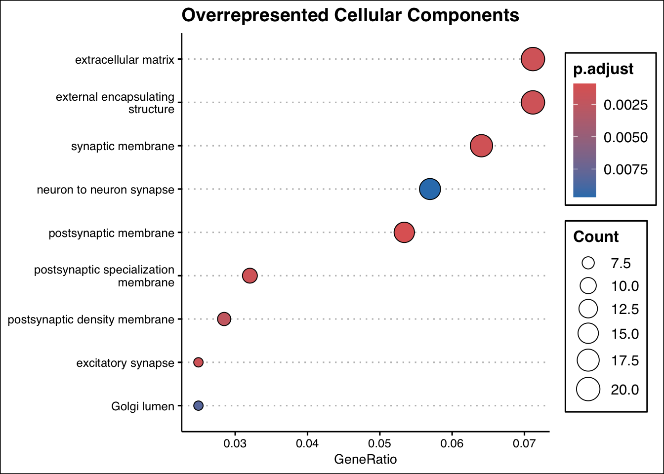
# ego_bp <- enrichGO(
#   gene = gene_entrez,
#   universe = names(geneList_entrez),
#   OrgDb = org.Hs.eg.db,
#   ont = "BP",
#   pAdjustMethod = "BH",
#   pvalueCutoff = 0.01,
#   qvalueCutoff = 0.05,
#   readable = TRUE
# )
#
# # Plot results
# dotplot(ego_bp, showCategory = 10, title = "Overrepresented Biological Processes") + ggthemes::theme_clean()
ego_mf <- enrichGO(
gene = gene_entrez,
universe = names(geneList_entrez),
OrgDb = org.Hs.eg.db,
ont = "MF",
pAdjustMethod = "BH",
pvalueCutoff = 0.01,
qvalueCutoff = 0.05,
readable = TRUE
)
# Plot results
dotplot(ego_mf, showCategory = 10, title = "Overrepresented Molecular Functions") + ggthemes::theme_clean()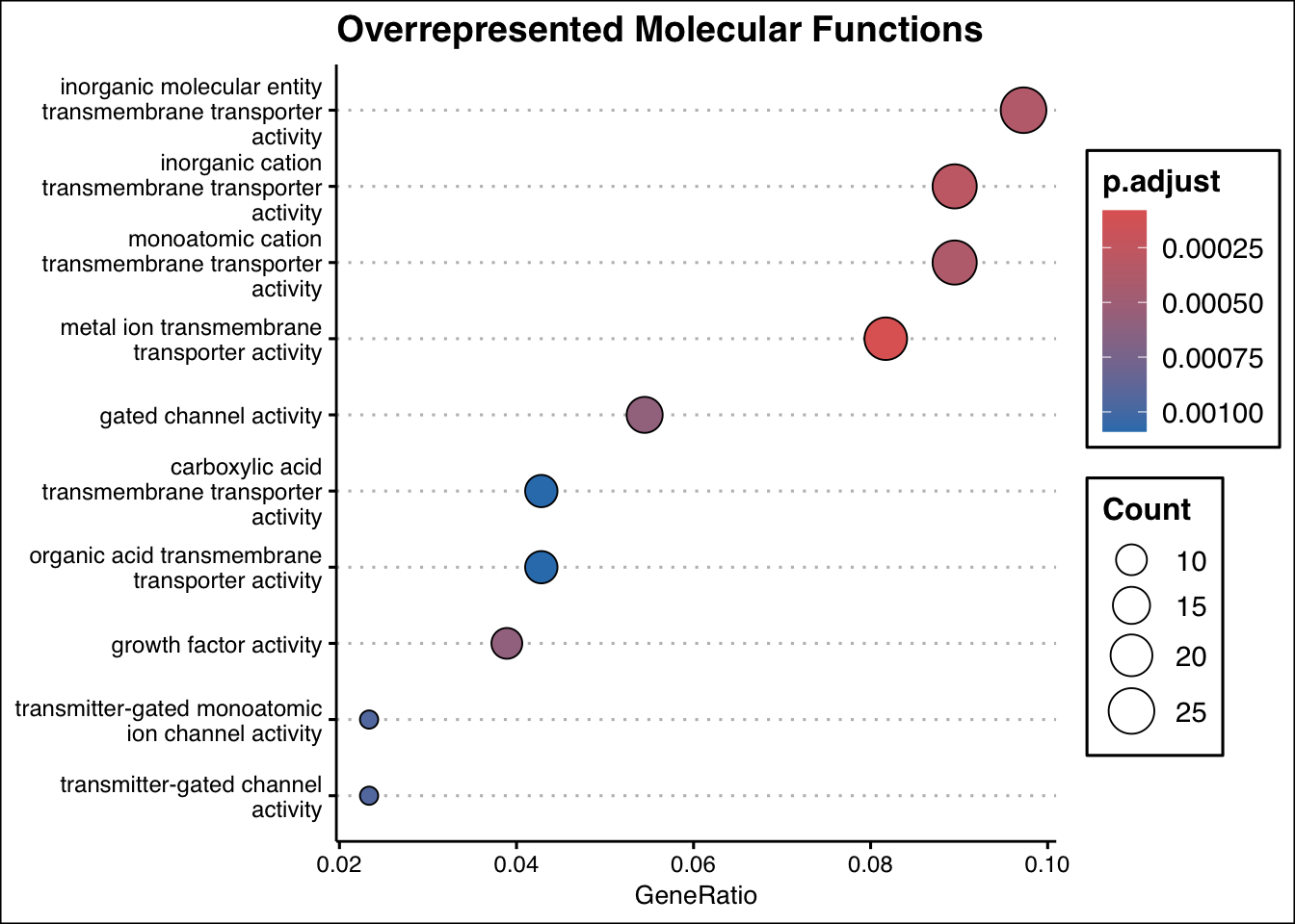
gl <- geneList_entrez[abs(geneList_entrez) > 2]
gl <- na.omit(gl)
gl_sorted <- sort(gl, decreasing = TRUE)

gse <- gseGO(
  geneList = gl_sorted,
  OrgDb = org.Hs.eg.db,
  ont = "ALL",
  minGSSize = 3,
  maxGSSize = 500,
  pvalueCutoff = 0.05,
  verbose = FALSE
)

dotplot(gse, showCategory = 10, split = ".sign", title = "GO Gene Set Enrichment Analysis") + facet_grid(. ~ .sign)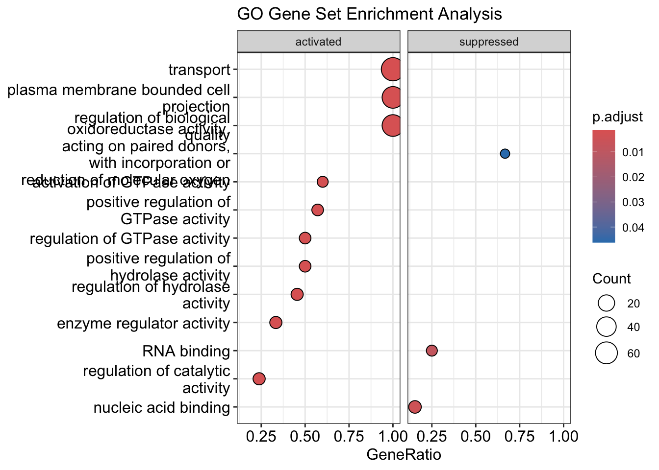
kk2 <- gseKEGG(
  geneList = gl_sorted,
  organism = "hsa", # humans = hsa for KEGG
  nPerm = 100000,
  minGSSize = 3,
  maxGSSize = 800,
  pvalueCutoff = 0.05,
  pAdjustMethod = "none",
  keyType = "ncbi-geneid"
)

dotplot(kk2, showCategory = 10, title = "Enriched KEGG Pathways", split = ".sign") + facet_grid(. ~ .sign)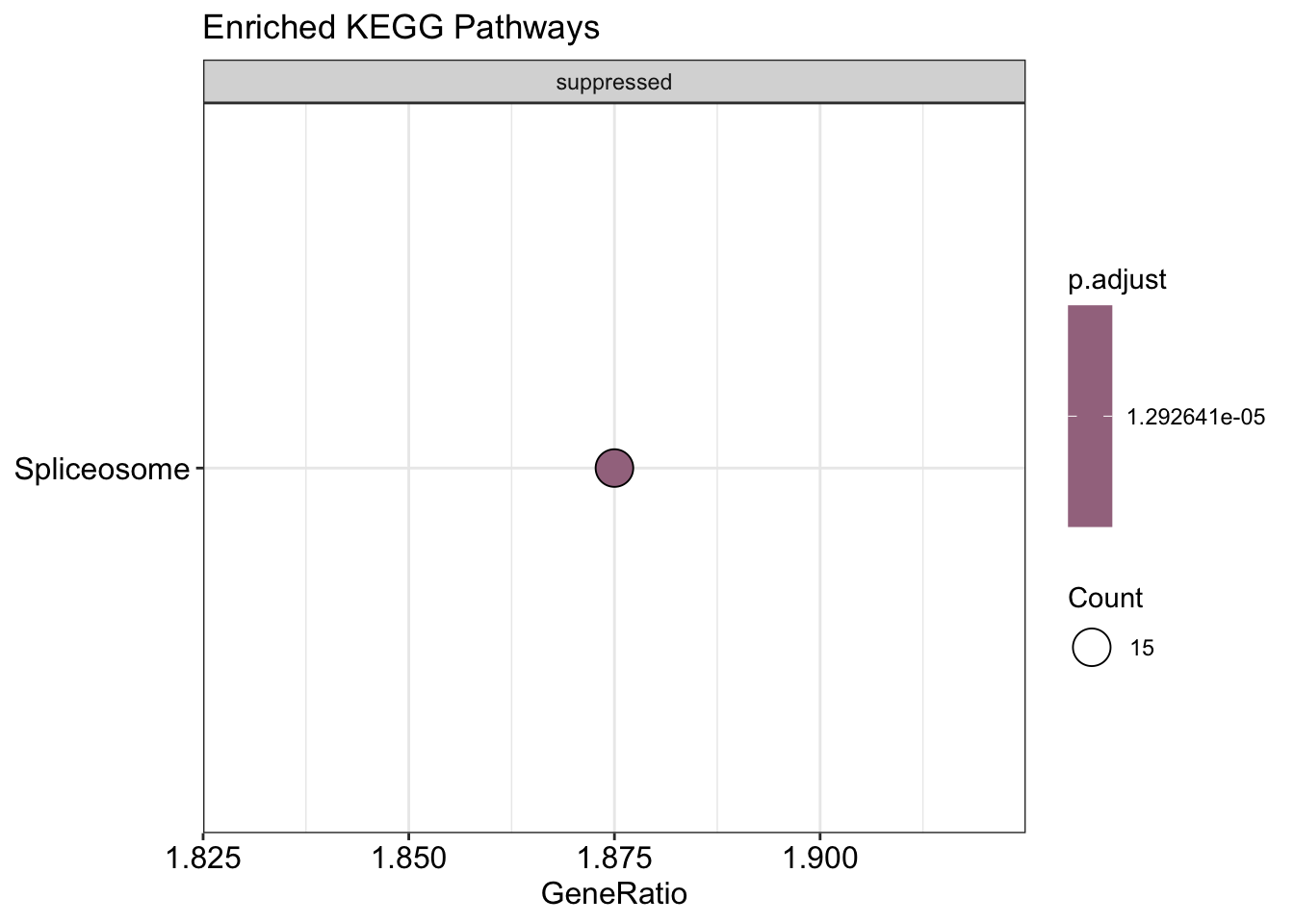
y <- enrichPathway(gene_entrez, pvalueCutoff = 0.05)

dotplot(y, showCategory = 10, title = "Reactome Pathway Over-representation Analysis", font.size = 10)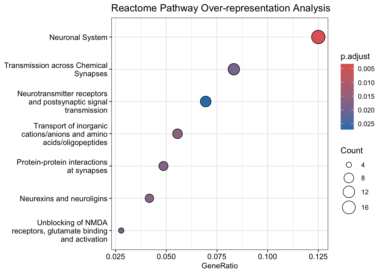
string_db <- STRINGdb$new(version = "11.5", species = 9606, score_threshold = 100, network_type = "full", input_directory = "")

mapped_degs <- string_db$map(significant_data, "name", removeUnmappedRows = TRUE)
Warning: we couldn't map to STRING 40% of your identifiershits <- mapped_degs$STRING_id[1:29]
mapped_degs_dec <- string_db$add_diff_exp_color(mapped_degs, logFcColStr = "lfc")
payload_id <- string_db$post_payload(mapped_degs_dec$STRING_id, colors = mapped_degs_dec$color)
string_db$plot_network(hits, payload_id = payload_id)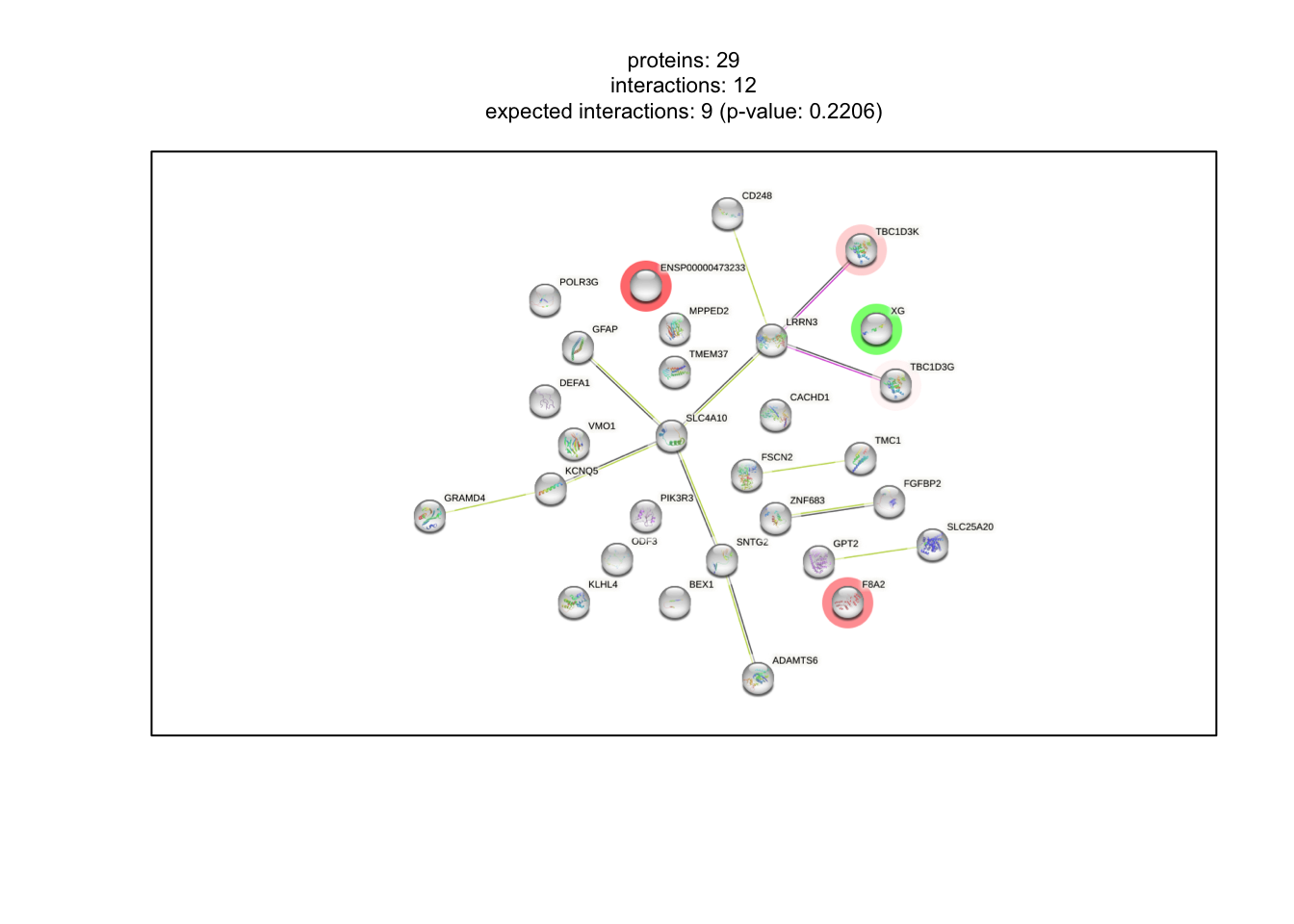
string_db <- STRINGdb$new(version = "11.5", species = 9606, score_threshold = 200, network_type = "full", input_directory = "")

significant_data_copy <- significant_data %>%
  rename(gene_name = name, log2FoldChange = lfc, baseMean = mean)

# Ensure both dataframes have the same columns (optional step to demonstrate alignment)
# This step is not necessary if you are sure both dataframes are already aligned
significant_data_copy <- significant_data_copy[c("gene_name", "baseMean", "log2FoldChange")]
filtered_by_interest2 <- filtered_by_interest[c("gene_name", "baseMean", "log2FoldChange")]

combined_df <- dplyr::bind_rows(significant_data_copy, filtered_by_interest2)

combined_df_mapped <- string_db$map(combined_df, "gene_name", removeUnmappedRows = TRUE)
Warning: we couldn't map to STRING 23% of your identifierscombined_hits <- combined_df_mapped$STRING_id
string_db$plot_network(combined_hits)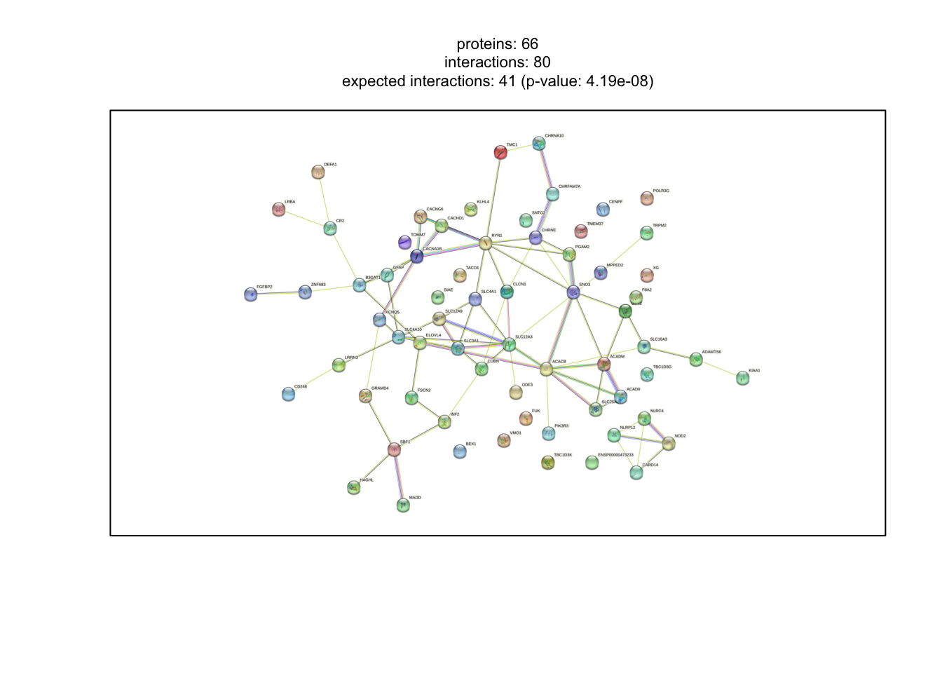
combined_enrichment <- string_db$get_enrichment(combined_hits)

enrich_file_name <- "output/stringdb_combined_enrichment.csv"
write.csv(combined_enrichment, enrich_file_name, row.names = FALSE)
listEnrichrSites()
setEnrichrSite("Enrichr") # Human genes
dbs <- listEnrichrDbs()
#query_dbs <- c("GO_Molecular_Function_2015", "GO_Cellular_Component_2015", "GO_Biological_Process_2015")
enriched <- enrichr(genes = significant_data$name, databases = dbs$libraryName)Uploading data to Enrichr... Done.
Querying Genome_Browser_PWMs... Done.
Querying TRANSFAC_and_JASPAR_PWMs... Done.
Querying Transcription_Factor_PPIs... Done.
Querying ChEA_2013... Done.
Querying Drug_Perturbations_from_GEO_2014... Done.
Querying ENCODE_TF_ChIP-seq_2014... Done.
Querying BioCarta_2013... Done.
Querying Reactome_2013... Done.
Querying WikiPathways_2013... Done.
Querying Disease_Signatures_from_GEO_up_2014... Done.
Querying KEGG_2013... Done.
Querying TF-LOF_Expression_from_GEO... Done.
Querying TargetScan_microRNA... Done.
Querying PPI_Hub_Proteins... Done.
Querying GO_Molecular_Function_2015... Done.
Querying GeneSigDB... Done.
Querying Chromosome_Location... Done.
Querying Human_Gene_Atlas... Done.
Querying Mouse_Gene_Atlas... Done.
Querying GO_Cellular_Component_2015... Done.
Querying GO_Biological_Process_2015... Done.
Querying Human_Phenotype_Ontology... Done.
Querying Epigenomics_Roadmap_HM_ChIP-seq... Done.
Querying KEA_2013... Done.
Querying NURSA_Human_Endogenous_Complexome... Done.
Querying CORUM... Done.
Querying SILAC_Phosphoproteomics... Done.
Querying MGI_Mammalian_Phenotype_Level_3... Done.
Querying MGI_Mammalian_Phenotype_Level_4... Done.
Querying Old_CMAP_up... Done.
Querying Old_CMAP_down... Done.
Querying OMIM_Disease... Done.
Querying OMIM_Expanded... Done.
Querying VirusMINT... Done.
Querying MSigDB_Computational... Done.
Querying MSigDB_Oncogenic_Signatures... Done.
Querying Disease_Signatures_from_GEO_down_2014... Done.
Querying Virus_Perturbations_from_GEO_up... Done.
Querying Virus_Perturbations_from_GEO_down... Done.
Querying Cancer_Cell_Line_Encyclopedia... Done.
Querying NCI-60_Cancer_Cell_Lines... Done.
Querying Tissue_Protein_Expression_from_ProteomicsDB... Done.
Querying Tissue_Protein_Expression_from_Human_Proteome_Map... Done.
Querying HMDB_Metabolites... Done.
Querying Pfam_InterPro_Domains... Done.
Querying GO_Biological_Process_2013... Done.
Querying GO_Cellular_Component_2013... Done.
Querying GO_Molecular_Function_2013... Done.
Querying Allen_Brain_Atlas_up... Done.
Querying ENCODE_TF_ChIP-seq_2015... Done.
Querying ENCODE_Histone_Modifications_2015... Done.
Querying Phosphatase_Substrates_from_DEPOD... Done.
Querying Allen_Brain_Atlas_down... Done.
Querying ENCODE_Histone_Modifications_2013... Done.
Querying Achilles_fitness_increase... Done.
Querying Achilles_fitness_decrease... Done.
Querying MGI_Mammalian_Phenotype_2013... Done.
Querying BioCarta_2015... Done.
Querying HumanCyc_2015... Done.
Querying KEGG_2015... Done.
Querying NCI-Nature_2015... Done.
Querying Panther_2015... Done.
Querying WikiPathways_2015... Done.
Querying Reactome_2015... Done.
Querying ESCAPE... Done.
Querying HomoloGene... Done.
Querying Disease_Perturbations_from_GEO_down... Done.
Querying Disease_Perturbations_from_GEO_up... Done.
Querying Drug_Perturbations_from_GEO_down... Done.
Querying Genes_Associated_with_NIH_Grants... Done.
Querying Drug_Perturbations_from_GEO_up... Done.
Querying KEA_2015... Done.
Querying Gene_Perturbations_from_GEO_up... Done.
Querying Gene_Perturbations_from_GEO_down... Done.
Querying ChEA_2015... Done.
Querying dbGaP... Done.
Querying LINCS_L1000_Chem_Pert_up... Done.
Querying LINCS_L1000_Chem_Pert_down... Done.
Querying GTEx_Tissue_Expression_Down... Done.
Querying GTEx_Tissue_Expression_Up... Done.
Querying Ligand_Perturbations_from_GEO_down... Done.
Querying Aging_Perturbations_from_GEO_down... Done.
Querying Aging_Perturbations_from_GEO_up... Done.
Querying Ligand_Perturbations_from_GEO_up... Done.
Querying MCF7_Perturbations_from_GEO_down... Done.
Querying MCF7_Perturbations_from_GEO_up... Done.
Querying Microbe_Perturbations_from_GEO_down... Done.
Querying Microbe_Perturbations_from_GEO_up... Done.
Querying LINCS_L1000_Ligand_Perturbations_down... Done.
Querying LINCS_L1000_Ligand_Perturbations_up... Done.
Querying L1000_Kinase_and_GPCR_Perturbations_down... Done.
Querying L1000_Kinase_and_GPCR_Perturbations_up... Done.
Querying Reactome_2016... Done.
Querying KEGG_2016... Done.
Querying WikiPathways_2016... Done.
Querying ENCODE_and_ChEA_Consensus_TFs_from_ChIP-X... Done.
Querying Kinase_Perturbations_from_GEO_down... Done.
Querying Kinase_Perturbations_from_GEO_up... Done.
Querying BioCarta_2016... Done.
Querying HumanCyc_2016... Done.
Querying NCI-Nature_2016... Done.
Querying Panther_2016... Done.
Querying DrugMatrix... Done.
Querying ChEA_2016... Done.
Querying huMAP... Done.
Querying Jensen_TISSUES... Done.
Querying RNA-Seq_Disease_Gene_and_Drug_Signatures_from_GEO... Done.
Querying MGI_Mammalian_Phenotype_2017... Done.
Querying Jensen_COMPARTMENTS... Done.
Querying Jensen_DISEASES... Done.
Querying BioPlex_2017... Done.
Querying GO_Cellular_Component_2017... Done.
Querying GO_Molecular_Function_2017... Done.
Querying GO_Biological_Process_2017... Done.
Querying GO_Cellular_Component_2017b... Done.
Querying GO_Molecular_Function_2017b... Done.
Querying GO_Biological_Process_2017b... Done.
Querying ARCHS4_Tissues... Done.
Querying ARCHS4_Cell-lines... Done.
Querying ARCHS4_IDG_Coexp... Done.
Querying ARCHS4_Kinases_Coexp... Done.
Querying ARCHS4_TFs_Coexp... Done.
Querying SysMyo_Muscle_Gene_Sets... Done.
Querying miRTarBase_2017... Done.
Querying TargetScan_microRNA_2017... Done.
Querying Enrichr_Libraries_Most_Popular_Genes... Done.
Querying Enrichr_Submissions_TF-Gene_Coocurrence... Done.
Querying Data_Acquisition_Method_Most_Popular_Genes... Done.
Querying DSigDB... Done.
Querying GO_Biological_Process_2018... Done.
Querying GO_Cellular_Component_2018... Done.
Querying GO_Molecular_Function_2018... Done.
Querying TF_Perturbations_Followed_by_Expression... Done.
Querying Chromosome_Location_hg19... Done.
Querying NIH_Funded_PIs_2017_Human_GeneRIF... Done.
Querying NIH_Funded_PIs_2017_Human_AutoRIF... Done.
Querying Rare_Diseases_AutoRIF_ARCHS4_Predictions... Done.
Querying Rare_Diseases_GeneRIF_ARCHS4_Predictions... Done.
Querying NIH_Funded_PIs_2017_AutoRIF_ARCHS4_Predictions... Done.
Querying NIH_Funded_PIs_2017_GeneRIF_ARCHS4_Predictions... Done.
Querying Rare_Diseases_GeneRIF_Gene_Lists... Done.
Querying Rare_Diseases_AutoRIF_Gene_Lists... Done.
Querying SubCell_BarCode... Done.
Querying GWAS_Catalog_2019... Done.
Querying WikiPathways_2019_Human... Done.
Querying WikiPathways_2019_Mouse... Done.
Querying TRRUST_Transcription_Factors_2019... Done.
Querying KEGG_2019_Human... Done.
Querying KEGG_2019_Mouse... Done.
Querying InterPro_Domains_2019... Done.
Querying Pfam_Domains_2019... Done.
Querying DepMap_WG_CRISPR_Screens_Broad_CellLines_2019... Done.
Querying DepMap_WG_CRISPR_Screens_Sanger_CellLines_2019... Done.
Querying MGI_Mammalian_Phenotype_Level_4_2019... Done.
Querying UK_Biobank_GWAS_v1... Done.
Querying BioPlanet_2019... Done.
Querying ClinVar_2019... Done.
Querying PheWeb_2019... Done.
Querying DisGeNET... Done.
Querying HMS_LINCS_KinomeScan... Done.
Querying CCLE_Proteomics_2020... Done.
Querying ProteomicsDB_2020... Done.
Querying lncHUB_lncRNA_Co-Expression... Done.
Querying Virus-Host_PPI_P-HIPSTer_2020... Done.
Querying Elsevier_Pathway_Collection... Done.
Querying Table_Mining_of_CRISPR_Studies... Done.
Querying COVID-19_Related_Gene_Sets... Done.
Querying MSigDB_Hallmark_2020... Done.
Querying Enrichr_Users_Contributed_Lists_2020... Done.
Querying TG_GATES_2020... Done.
Querying Allen_Brain_Atlas_10x_scRNA_2021... Done.
Querying Descartes_Cell_Types_and_Tissue_2021... Done.
Querying KEGG_2021_Human... Done.
Querying WikiPathway_2021_Human... Done.
Querying HuBMAP_ASCT_plus_B_augmented_w_RNAseq_Coexpression... Done.
Querying GO_Biological_Process_2021... Done.
Querying GO_Cellular_Component_2021... Done.
Querying GO_Molecular_Function_2021... Done.
Querying MGI_Mammalian_Phenotype_Level_4_2021... Done.
Querying CellMarker_Augmented_2021... Done.
Querying Orphanet_Augmented_2021... Done.
Querying COVID-19_Related_Gene_Sets_2021... Done.
Querying PanglaoDB_Augmented_2021... Done.
Querying Azimuth_Cell_Types_2021... Done.
Querying PhenGenI_Association_2021... Done.
Querying RNAseq_Automatic_GEO_Signatures_Human_Down... Done.
Querying RNAseq_Automatic_GEO_Signatures_Human_Up... Done.
Querying RNAseq_Automatic_GEO_Signatures_Mouse_Down... Done.
Querying RNAseq_Automatic_GEO_Signatures_Mouse_Up... Done.
Querying GTEx_Aging_Signatures_2021... Done.
Querying HDSigDB_Human_2021... Done.
Querying HDSigDB_Mouse_2021... Done.
Querying HuBMAP_ASCTplusB_augmented_2022... Done.
Querying FANTOM6_lncRNA_KD_DEGs... Done.
Querying MAGMA_Drugs_and_Diseases... Done.
Querying PFOCR_Pathways... Done.
Querying Tabula_Sapiens... Done.
Querying ChEA_2022... Done.
Querying Diabetes_Perturbations_GEO_2022... Done.
Querying LINCS_L1000_Chem_Pert_Consensus_Sigs... Done.
Querying LINCS_L1000_CRISPR_KO_Consensus_Sigs... Done.
Querying Tabula_Muris... Done.
Querying Reactome_2022... Done.
Querying SynGO_2022... Done.
Querying GlyGen_Glycosylated_Proteins_2022... Done.
Querying IDG_Drug_Targets_2022... Done.
Querying KOMP2_Mouse_Phenotypes_2022... Done.
Querying Metabolomics_Workbench_Metabolites_2022... Done.
Querying Proteomics_Drug_Atlas_2023... Done.
Querying The_Kinase_Library_2023... Done.
Querying GTEx_Tissues_V8_2023... Done.
Querying GO_Biological_Process_2023... Done.
Querying GO_Cellular_Component_2023... Done.
Querying GO_Molecular_Function_2023... Done.
Querying PFOCR_Pathways_2023... Done.
Querying GWAS_Catalog_2023... Done.
Querying GeDiPNet_2023... Done.
Querying MAGNET_2023... Done.
Querying Azimuth_2023... Done.
Querying Rummagene_kinases... Done.
Querying Rummagene_signatures... Done.
Querying Rummagene_transcription_factors... Done.
Querying MoTrPAC_2023... Done.
Querying WikiPathway_2023_Human... Done.
Querying SynGO_2024... Done.
Querying CellMarker_2024... Done.
Parsing results... Done.db_names <- names(enriched)
for (db_name in db_names) {
df <- as.data.frame(enriched[[db_name]]) # Access the data frame by name
if (is.data.frame(df)) { # Ensure it is a data frame
file_name <- paste0("output/enrichr-dbs/", db_name, ".csv")
write.csv(df, file_name, row.names = FALSE) # Write to CSV without row names
}
}cluster <- list("Significant Genes" = gene_entrez2, "Genes of Interest" = as.character(results2$entrezgene_id))
ck <- compareCluster(geneCluster = cluster, fun = "enrichGO", OrgDb='org.Hs.eg.db')
ck <- setReadable(ck, OrgDb = org.Hs.eg.db, keyType="ENTREZID")
dotplot(ck)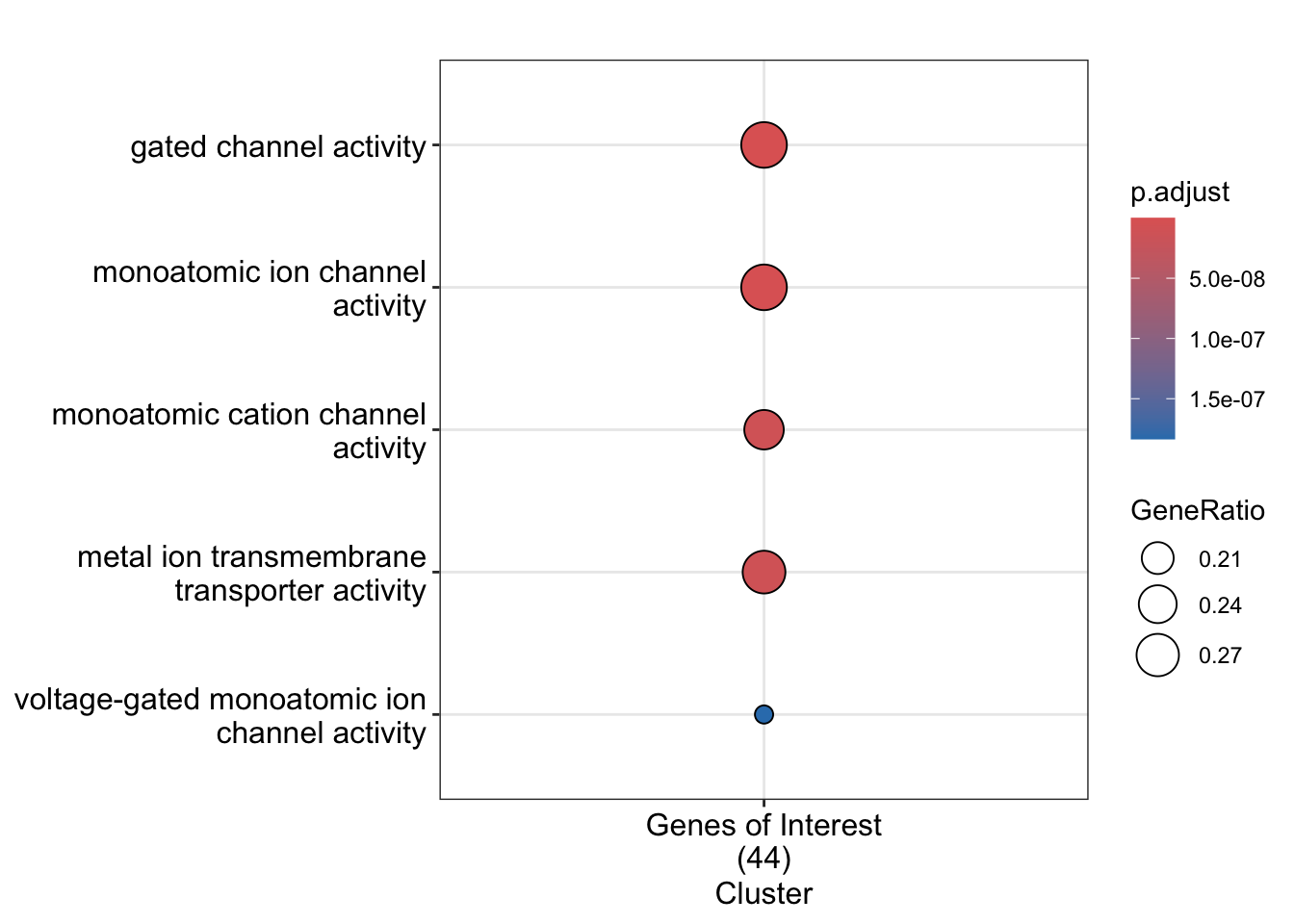
xx <- compareCluster(cluster, fun="enrichKEGG",
                     organism="hsa", pvalueCutoff=0.05)
dotplot(xx)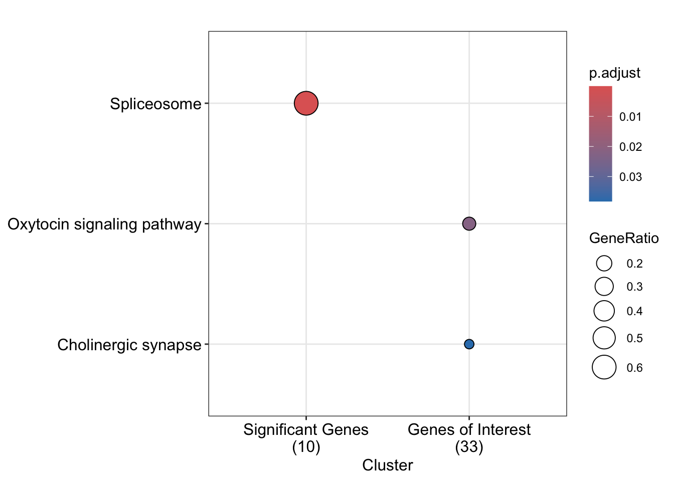
xx <- compareCluster(cluster, fun="enrichPathway", pvalueCutoff=0.05)
dotplot(xx)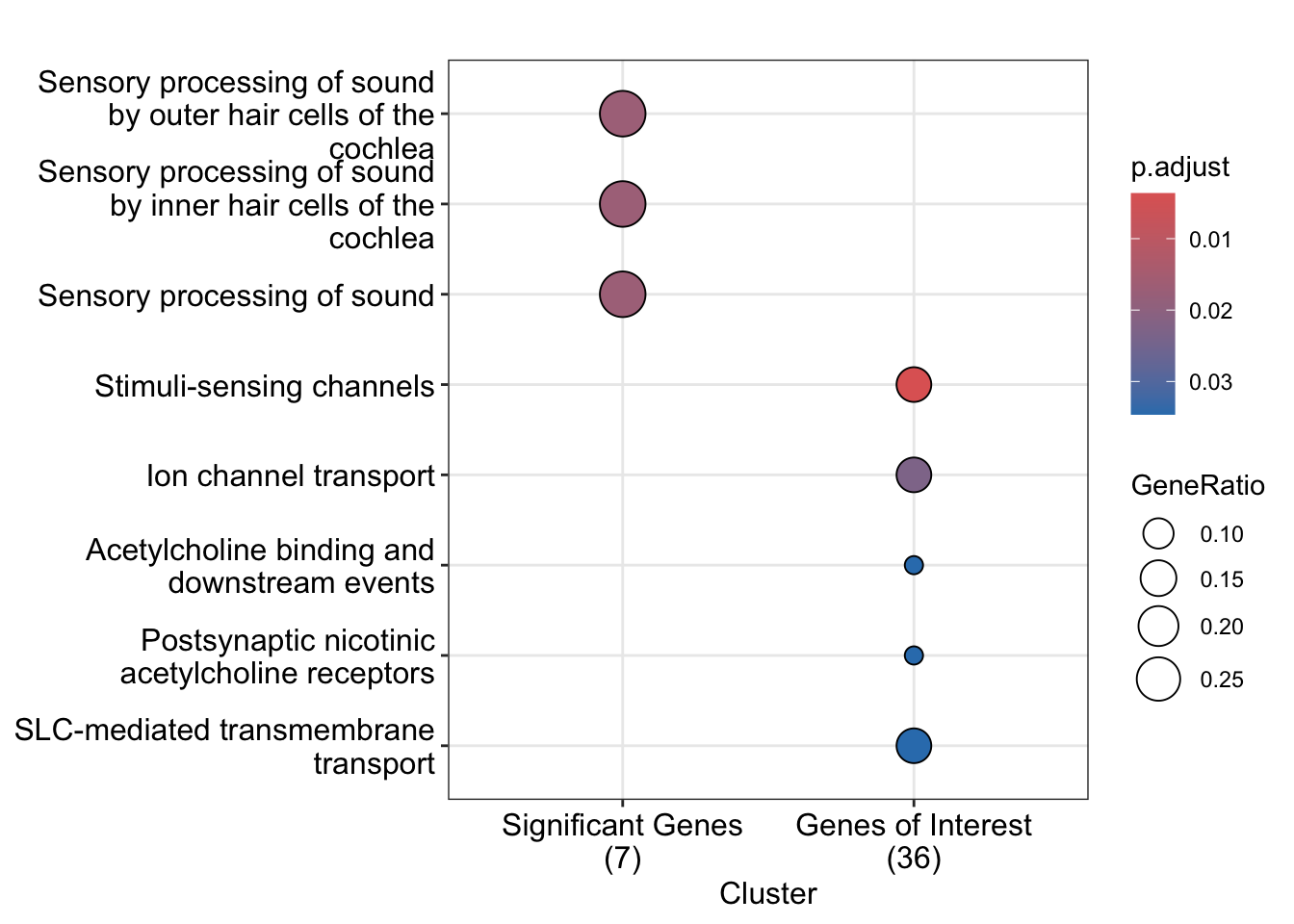
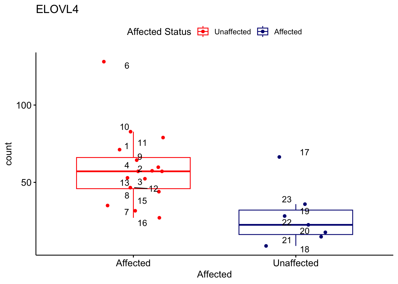
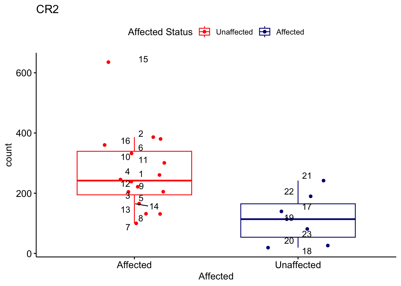
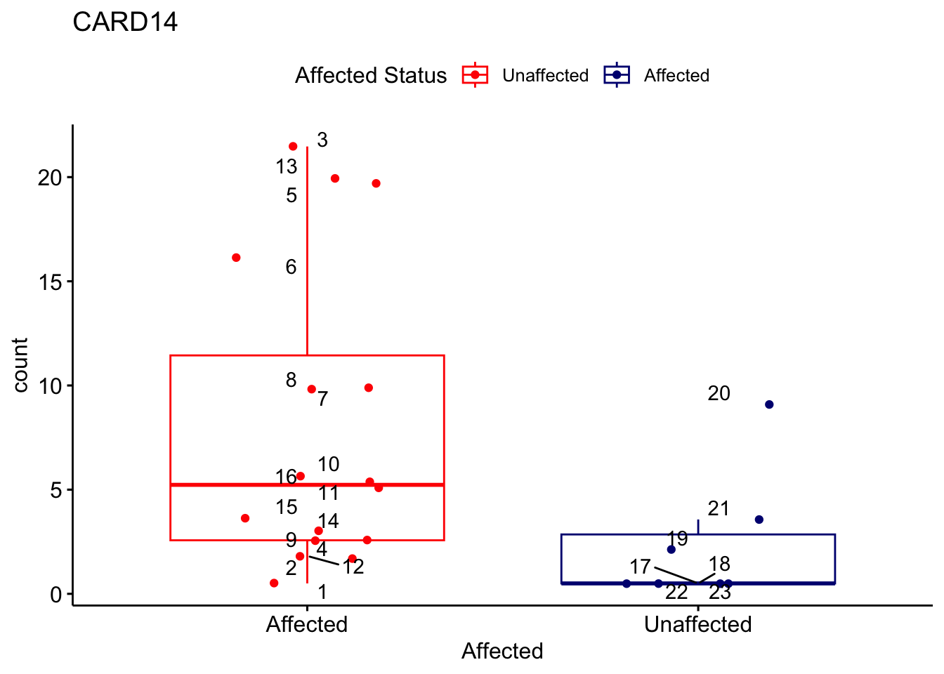
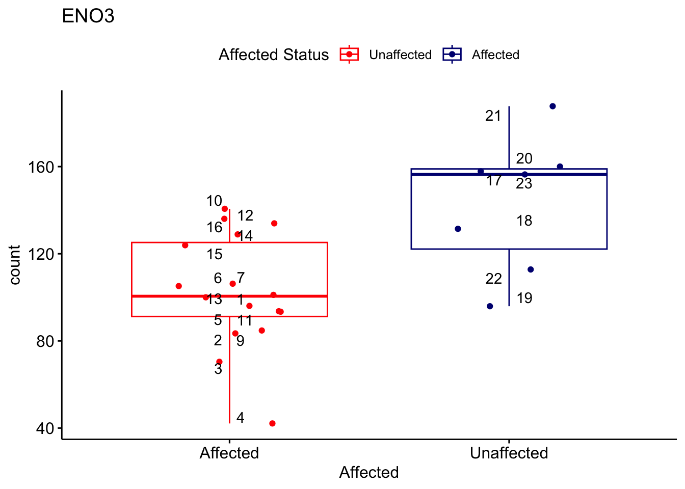
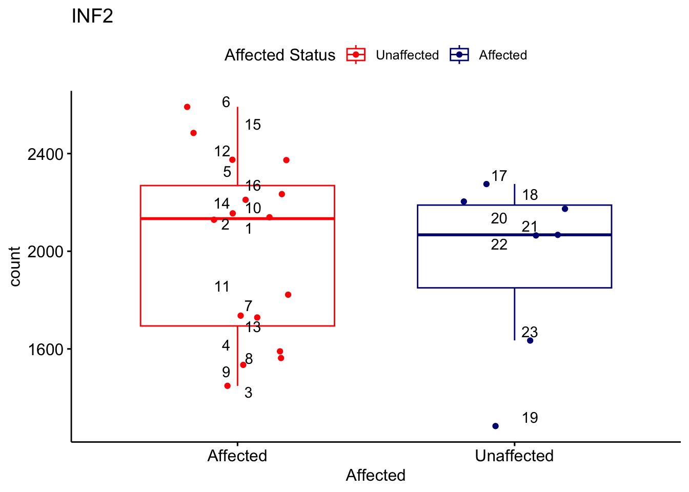
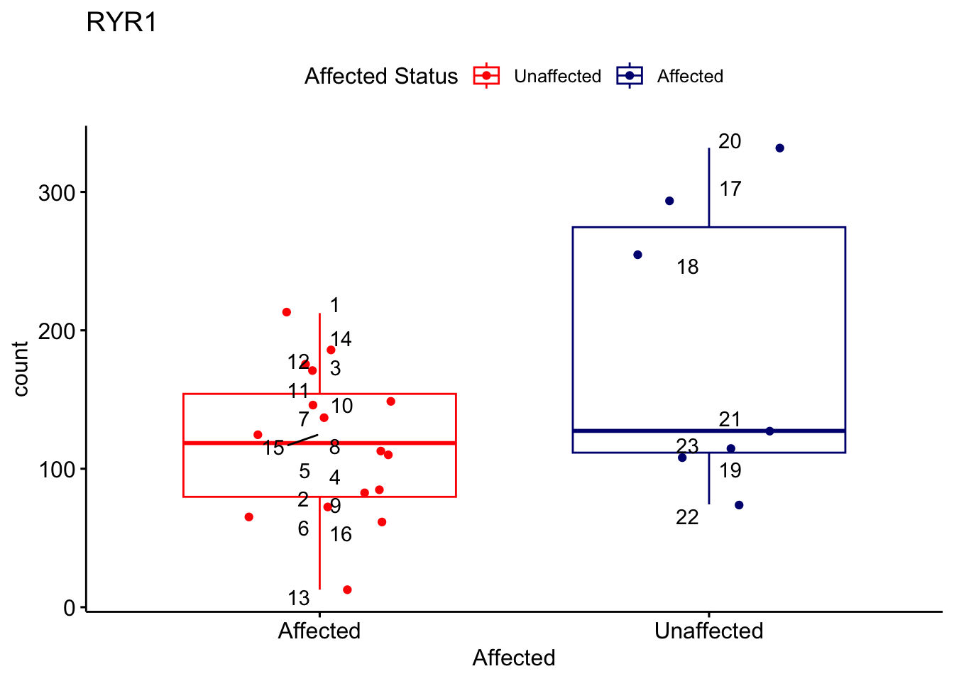
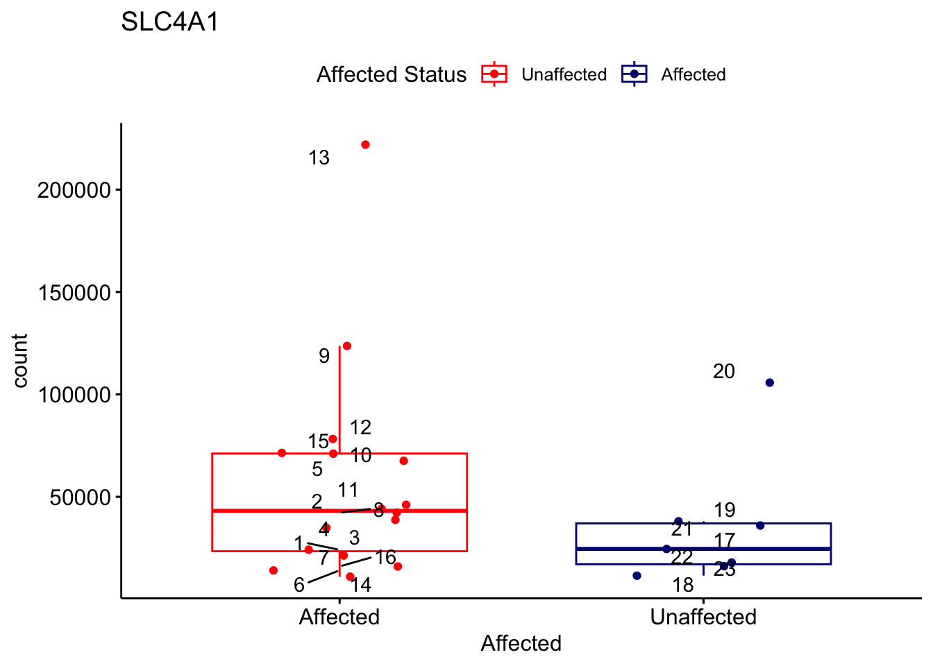
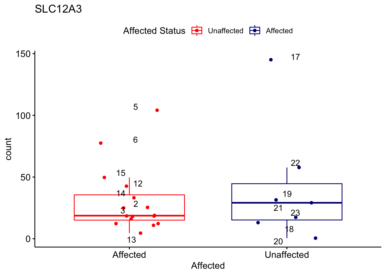
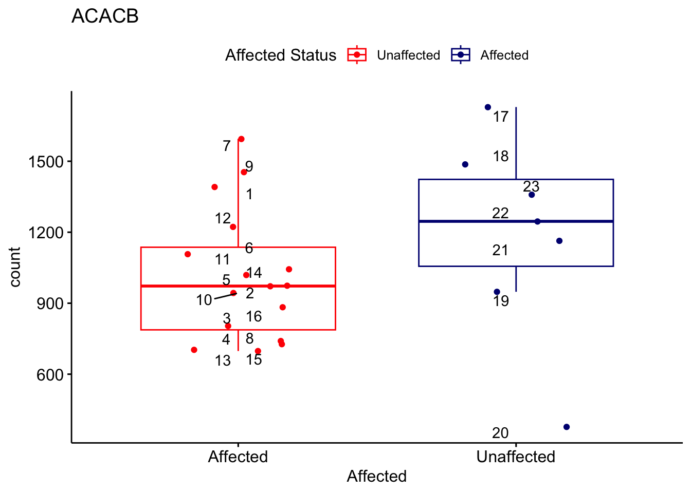
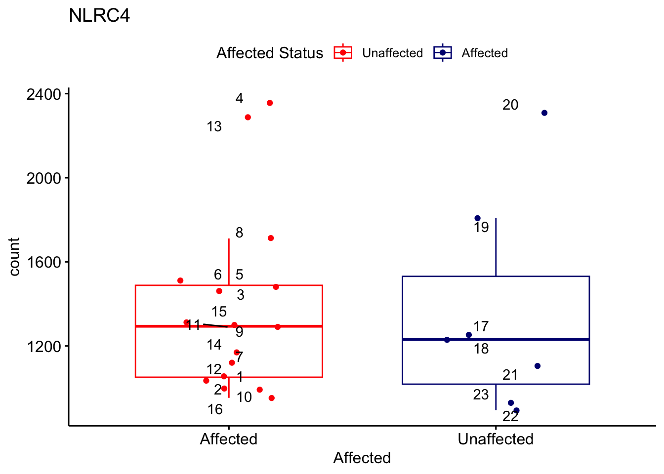
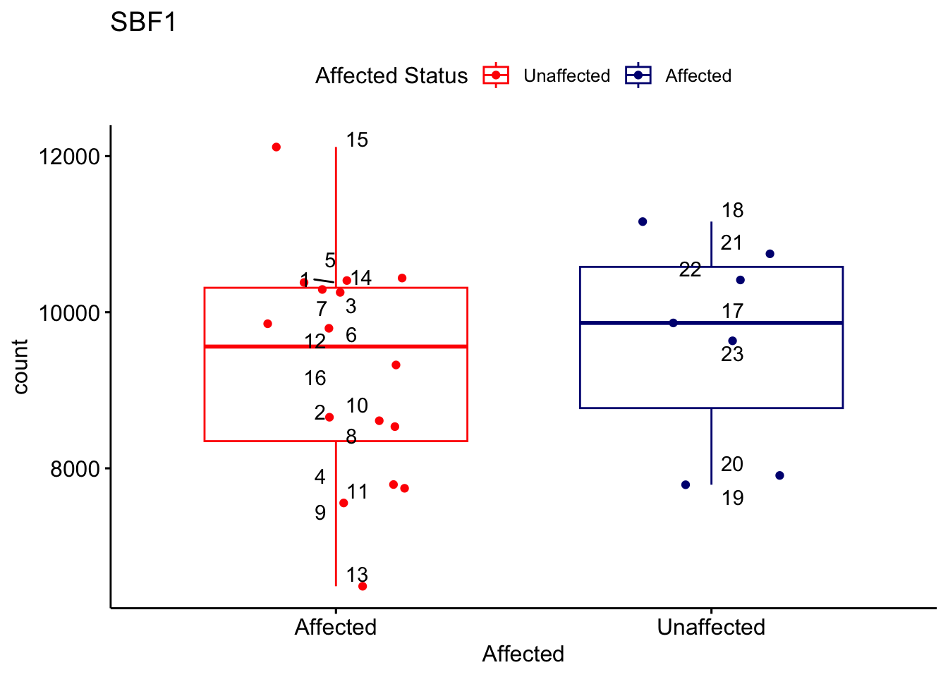
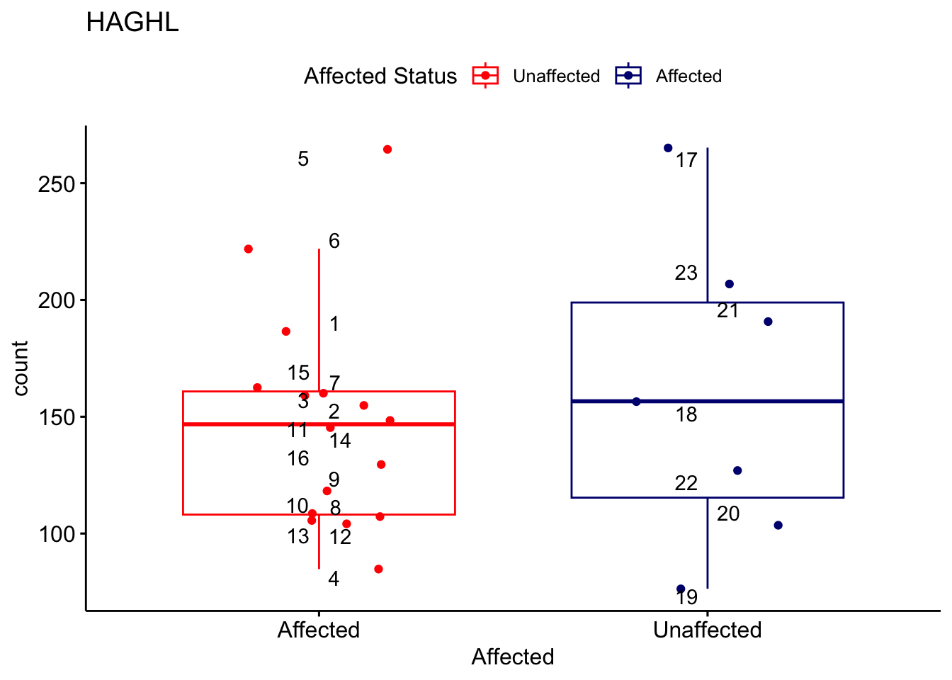
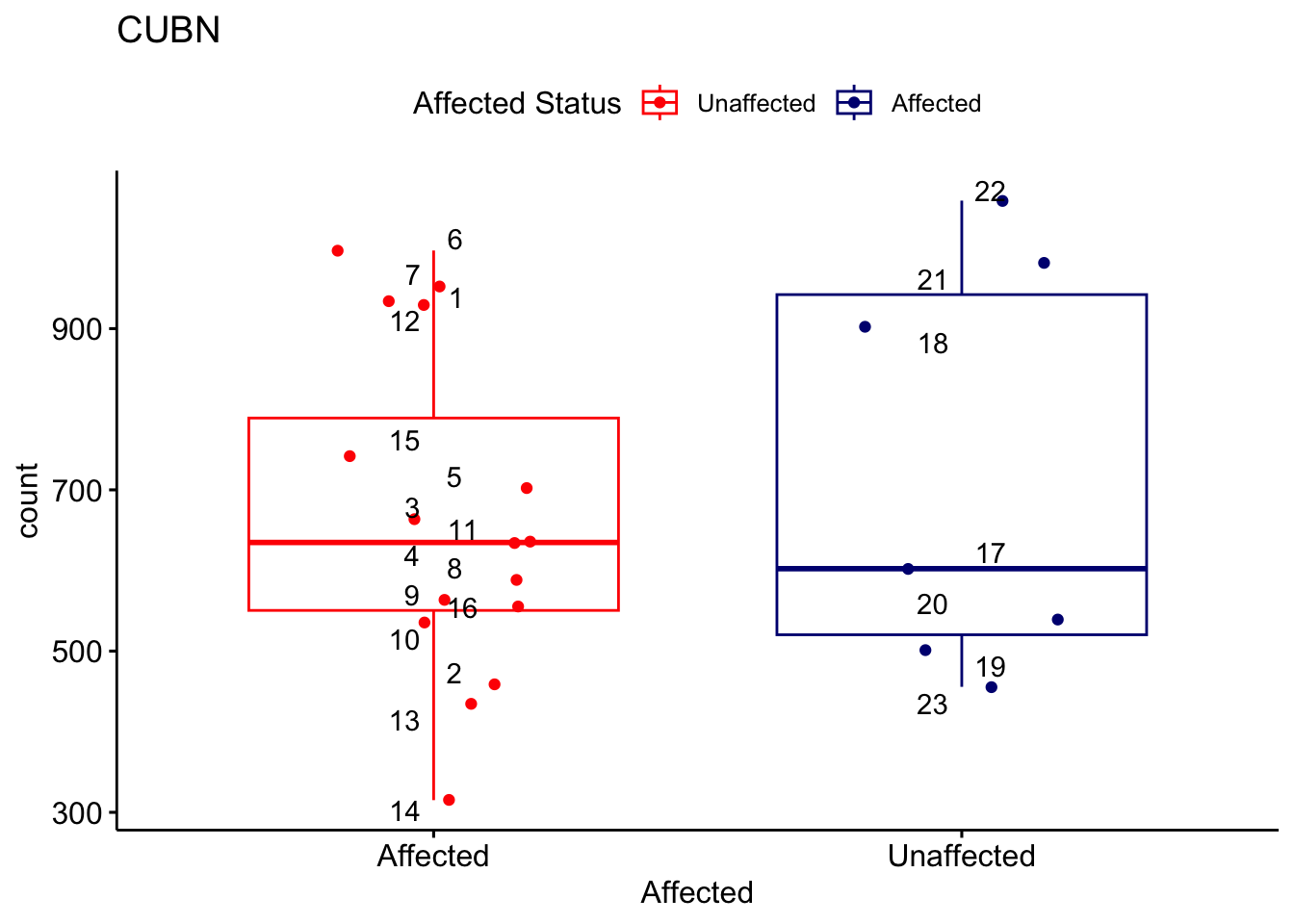
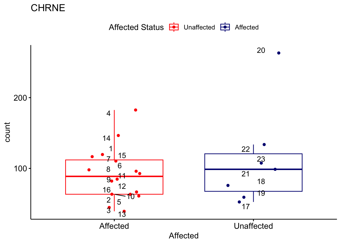
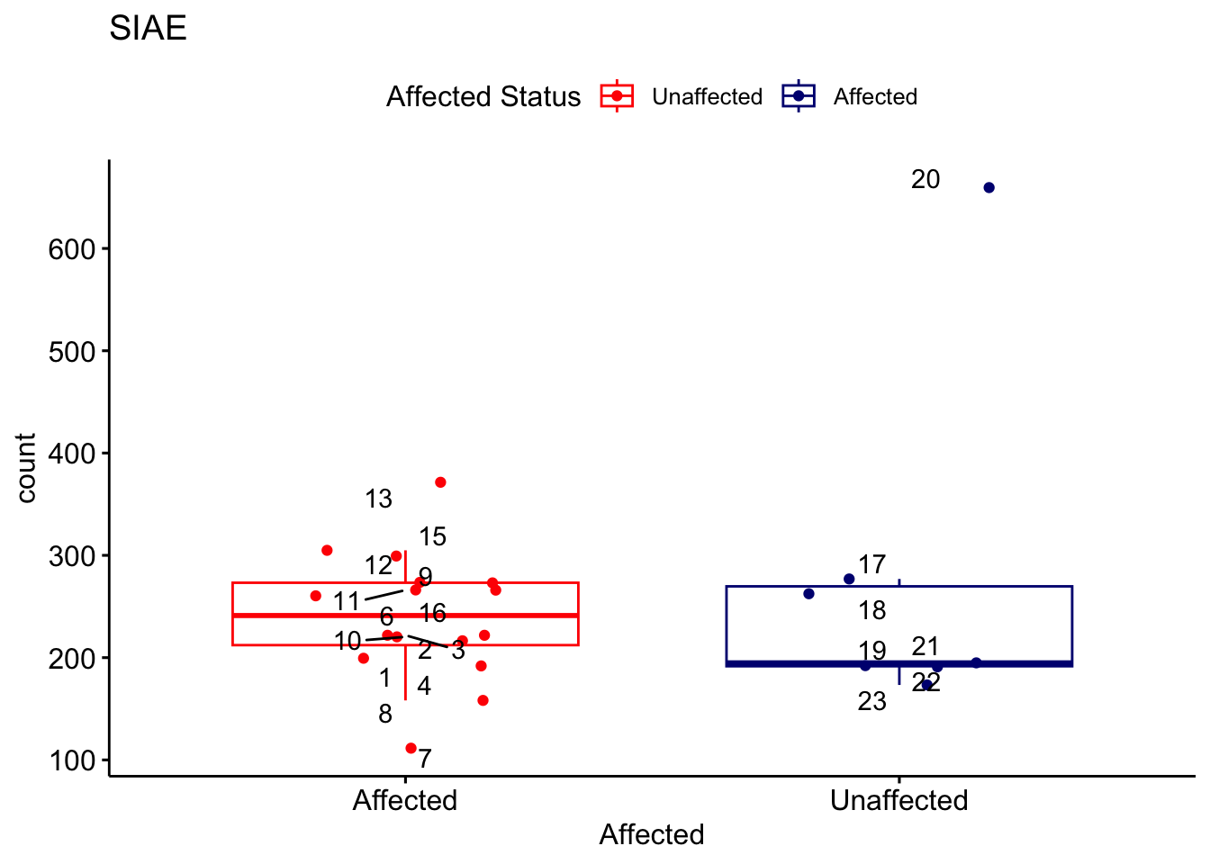
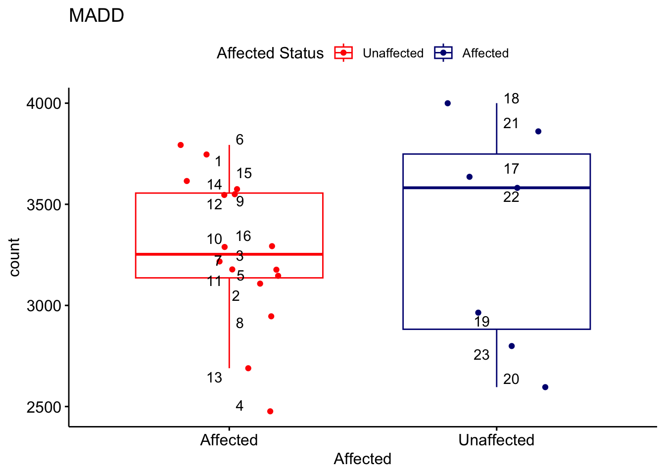
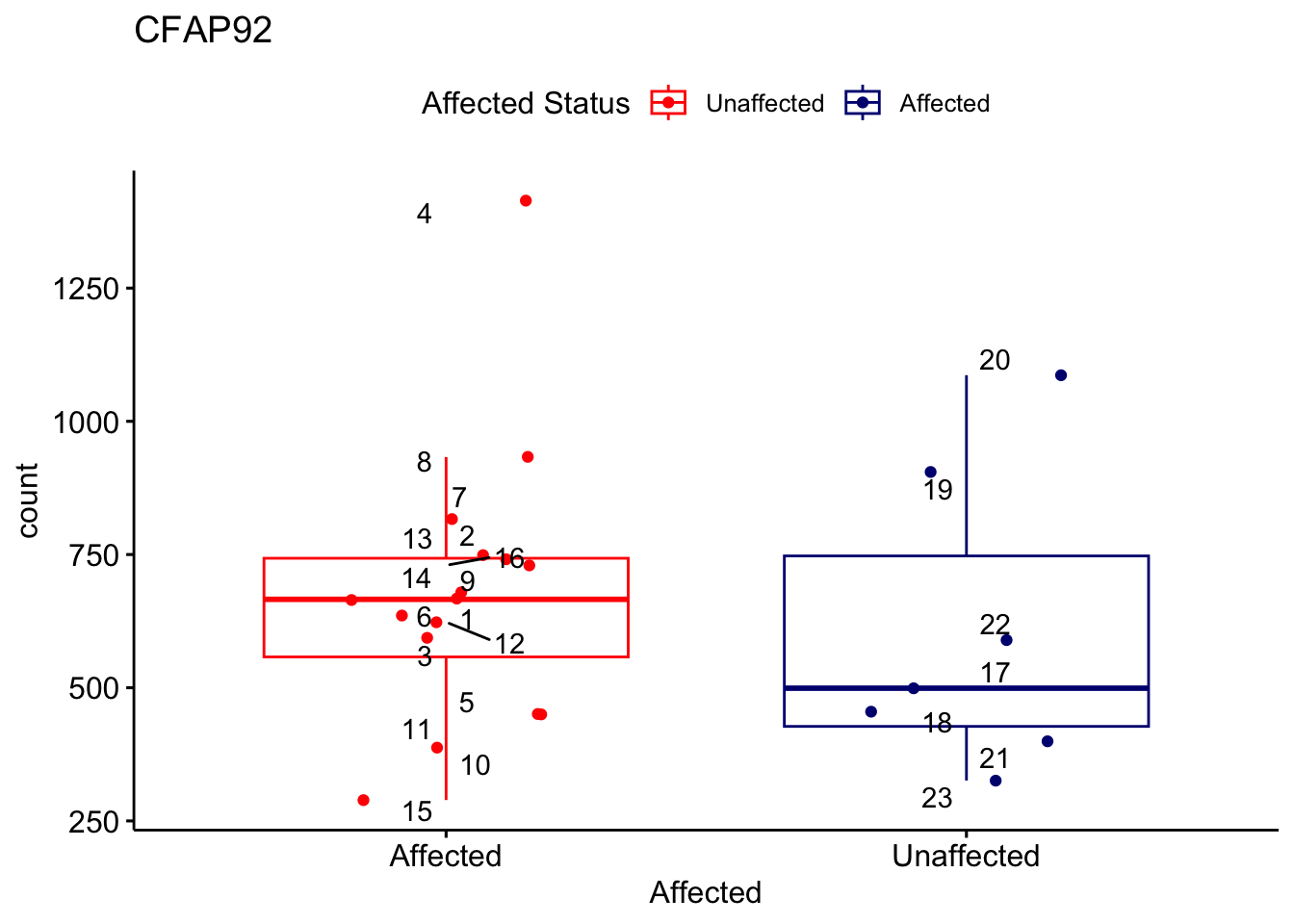
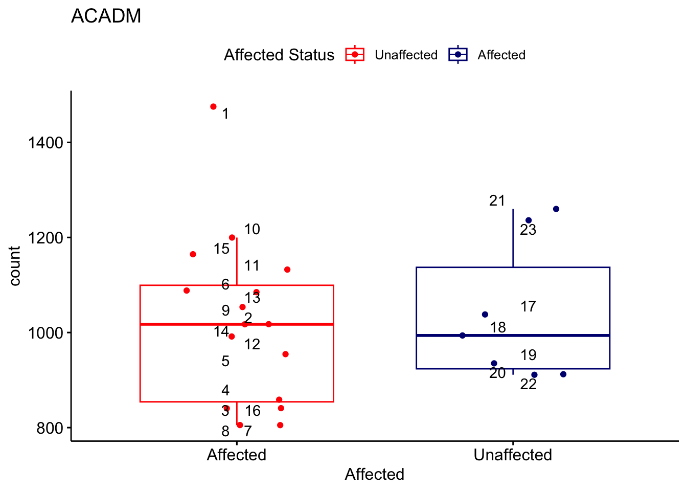
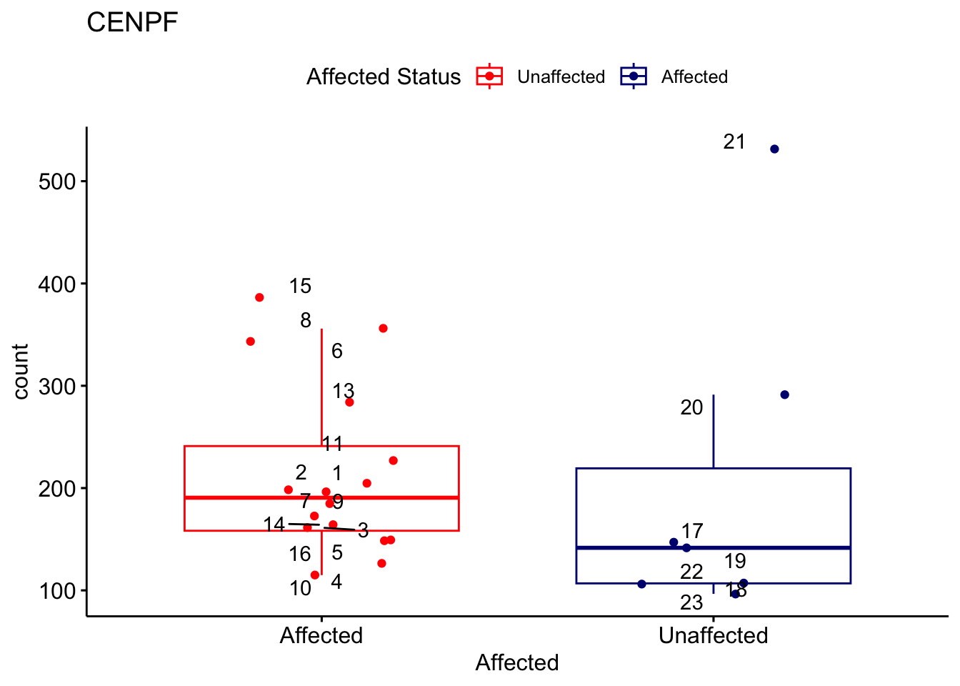
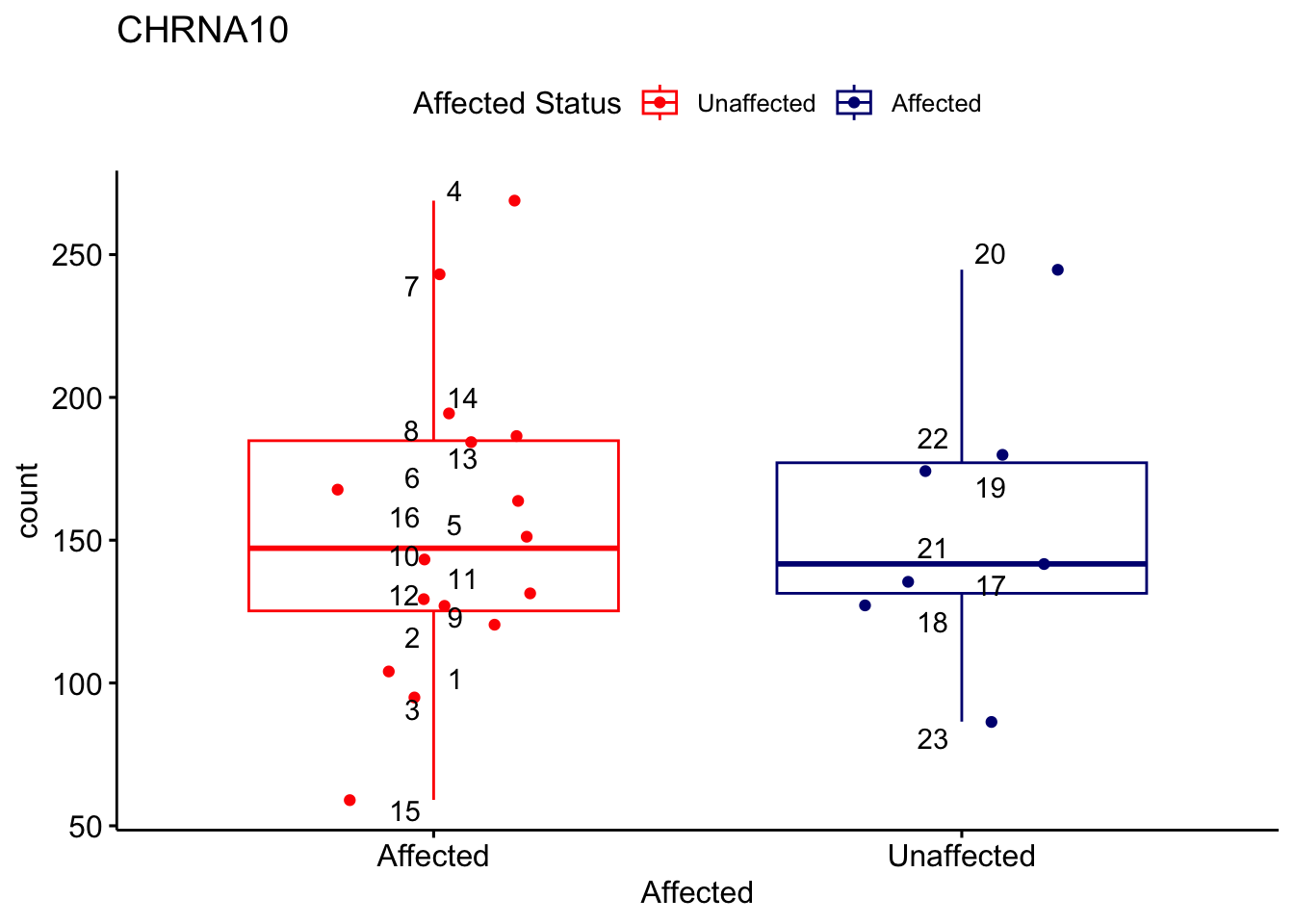
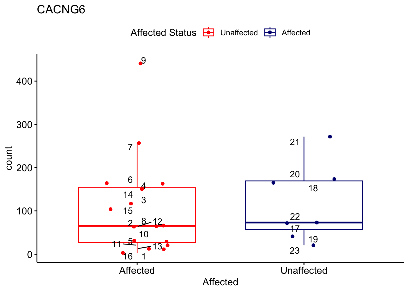
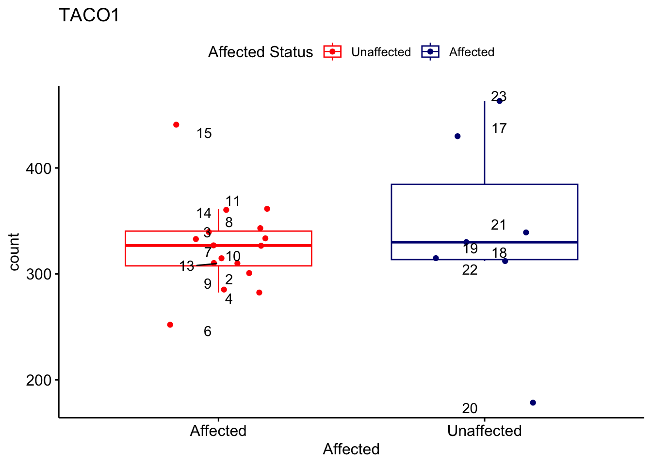
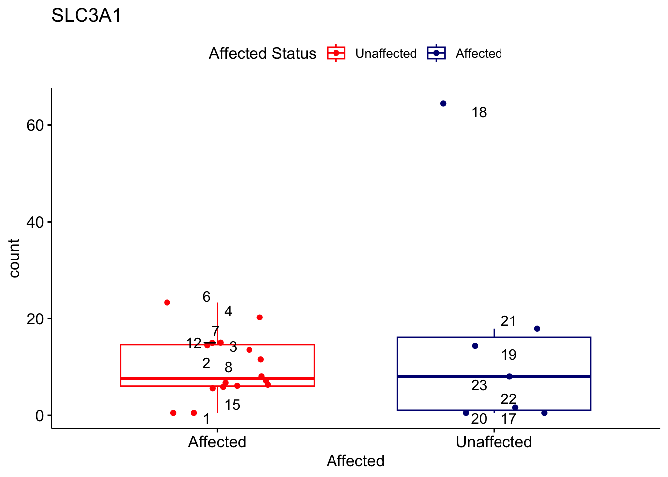
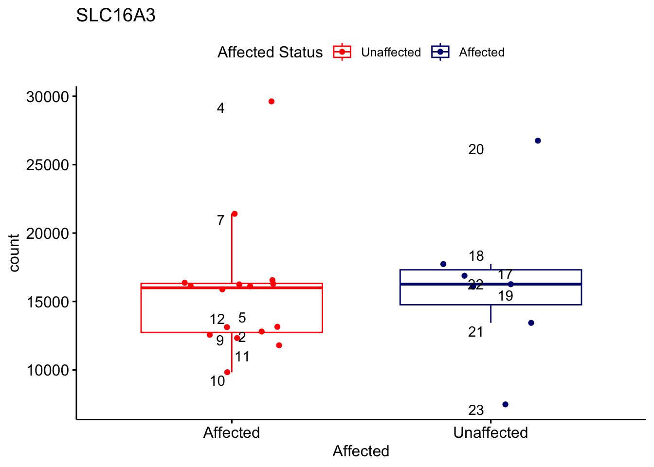
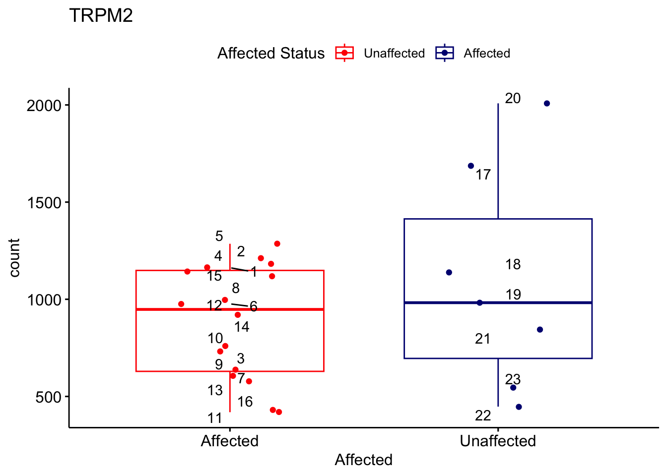
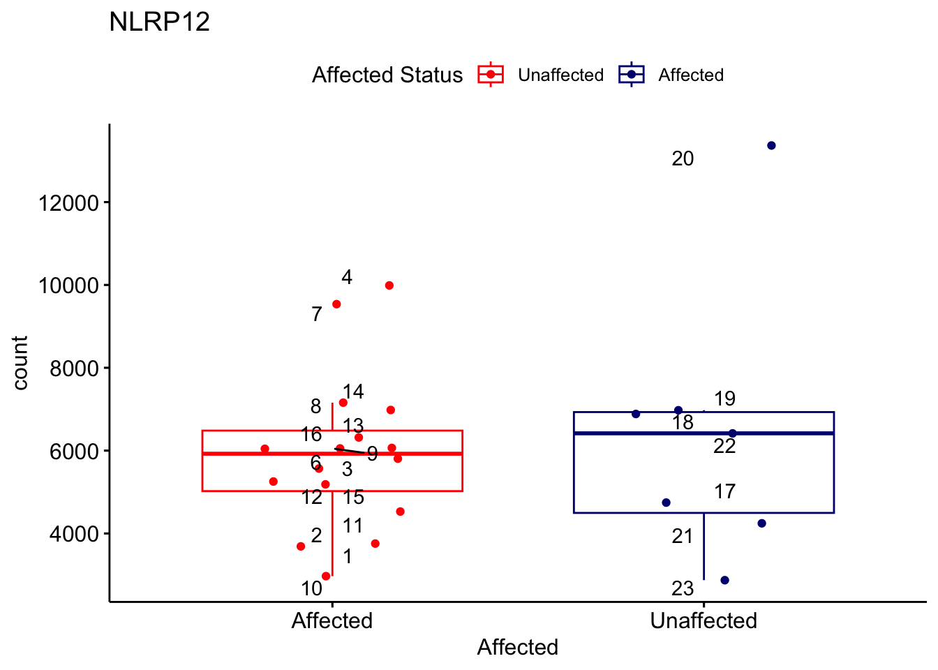
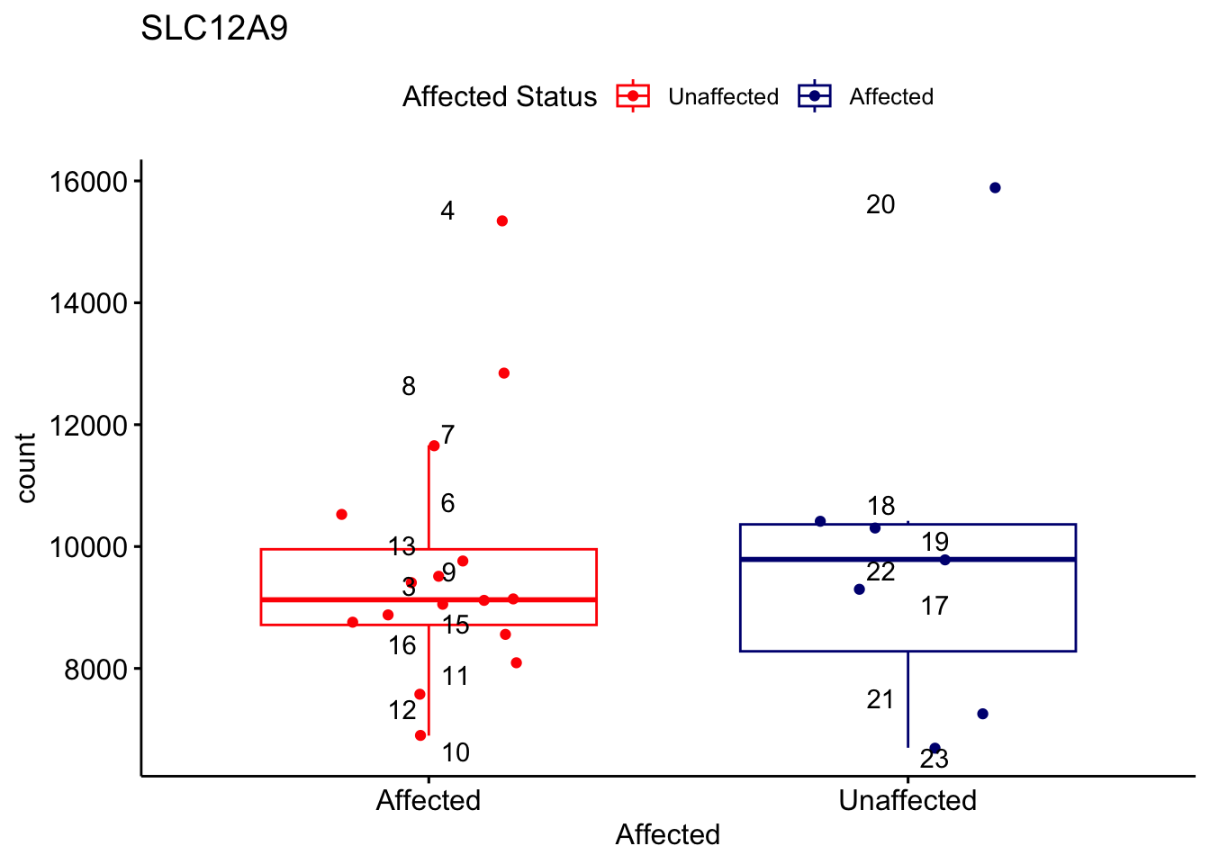
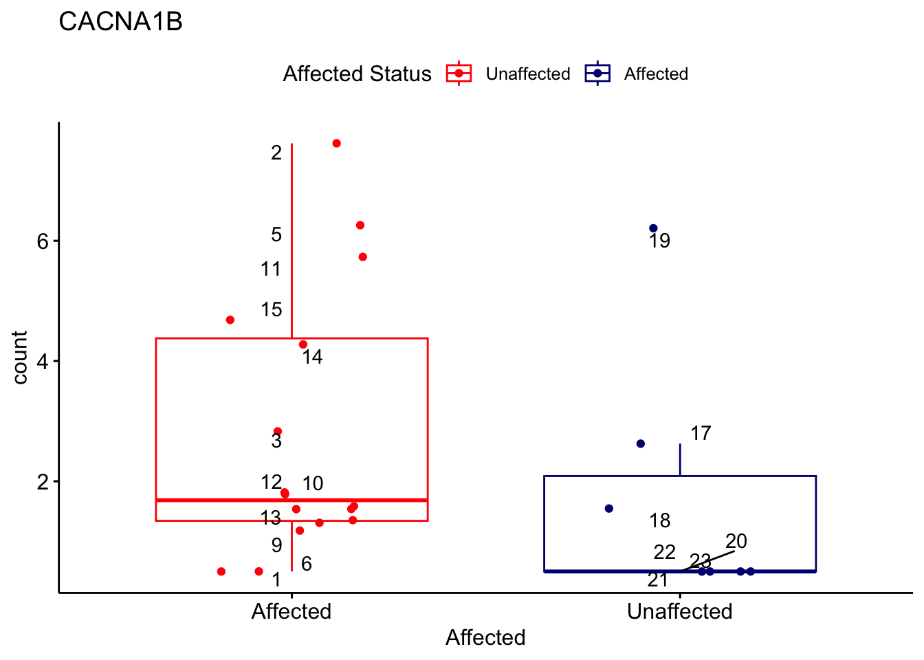
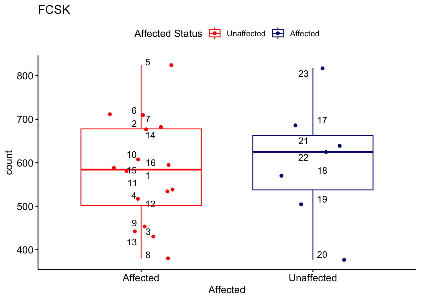
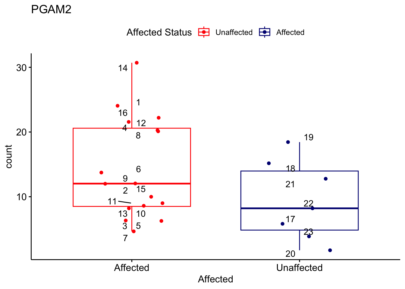
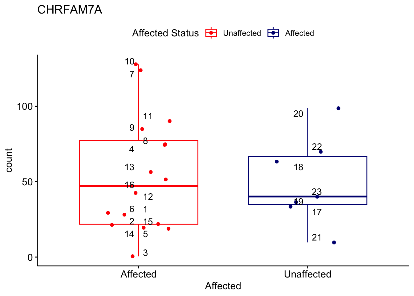
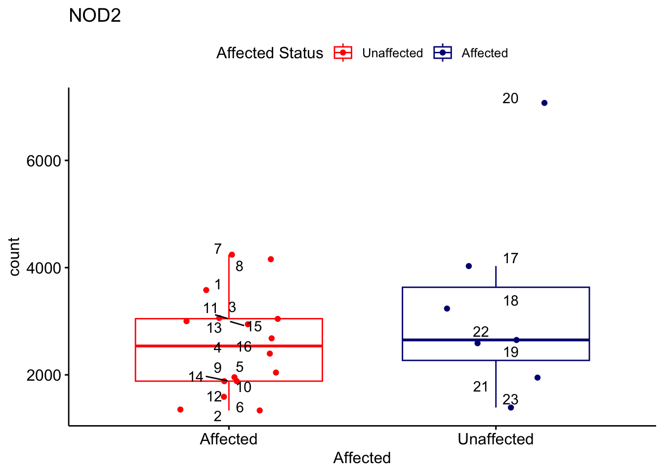
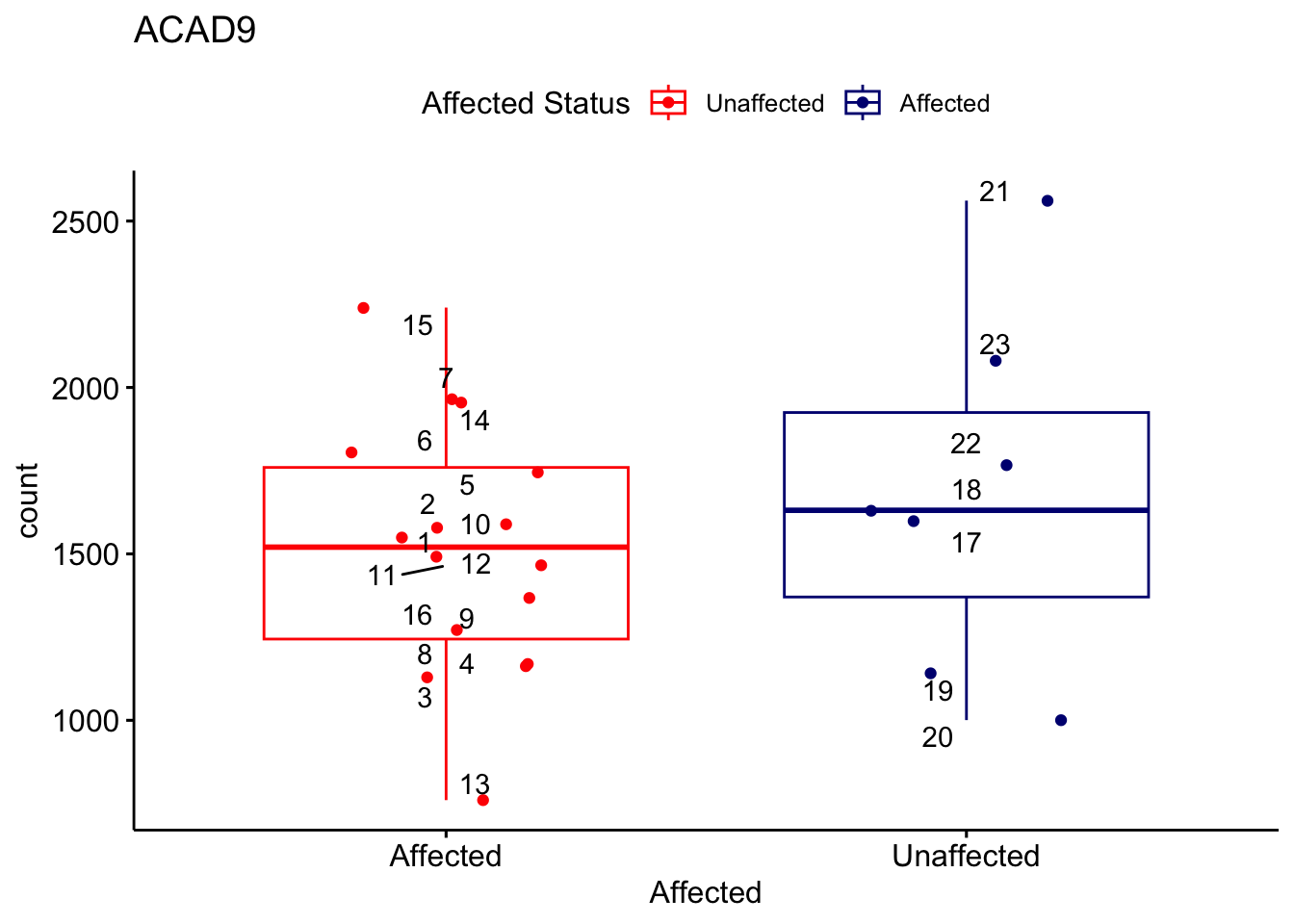
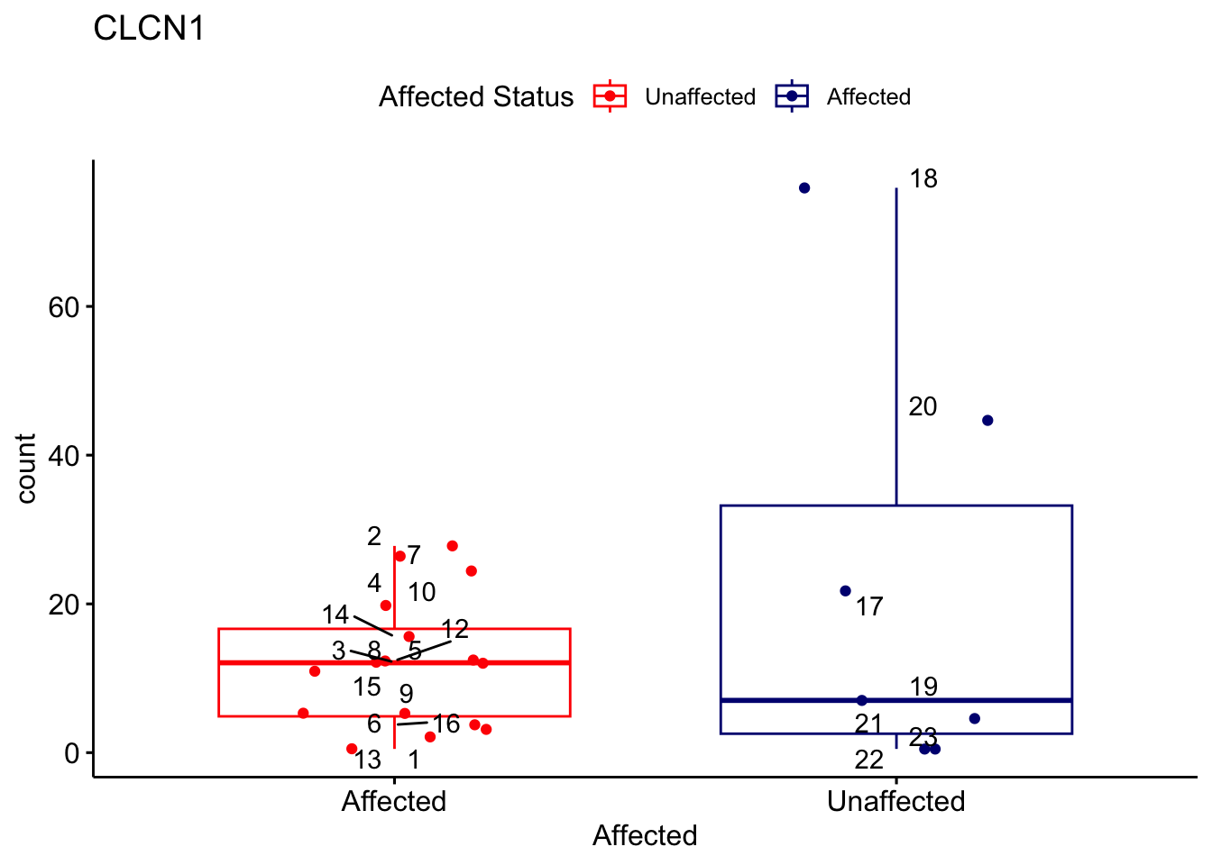
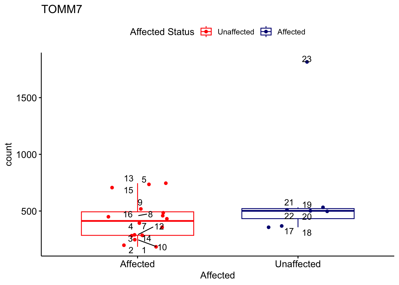
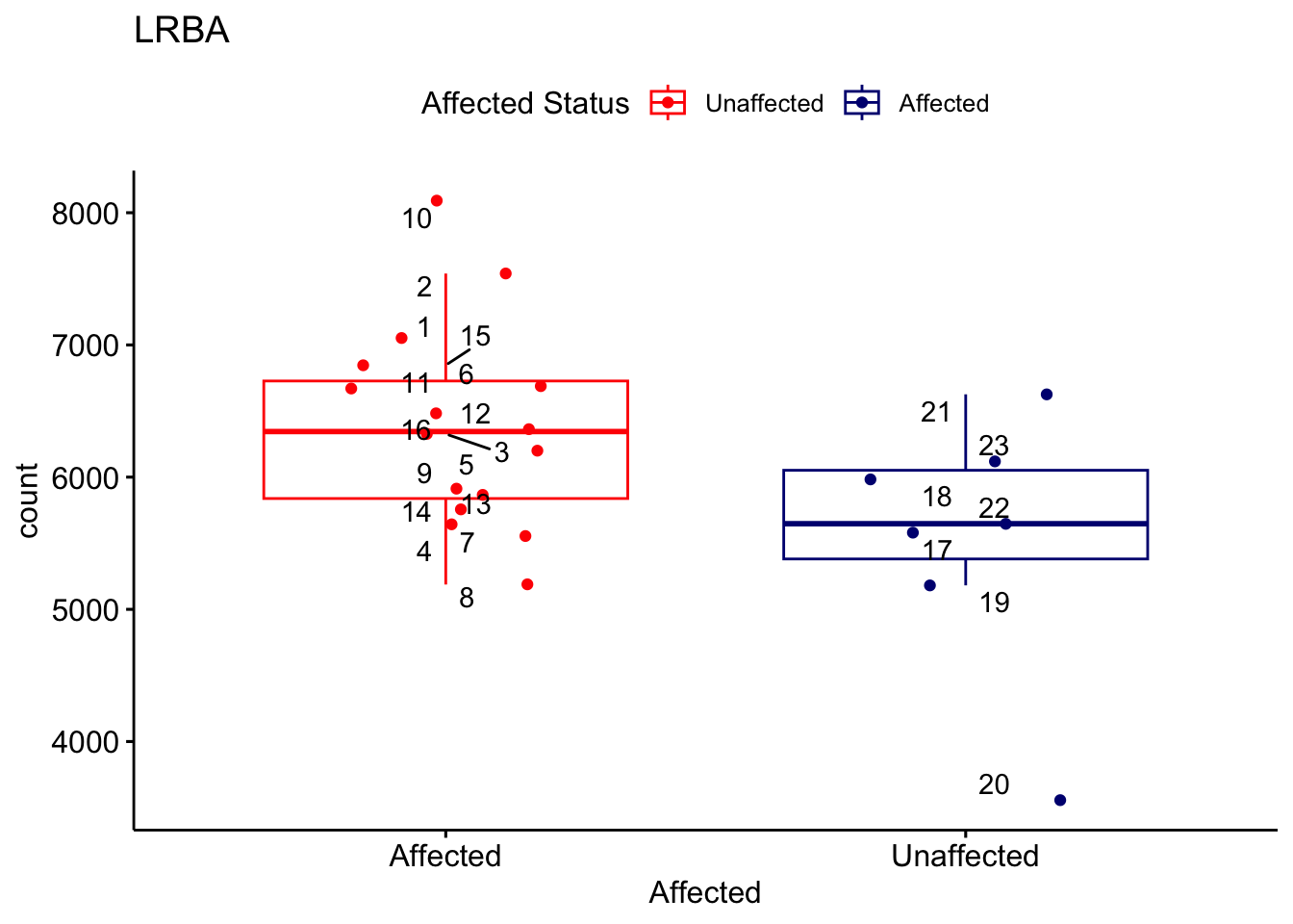
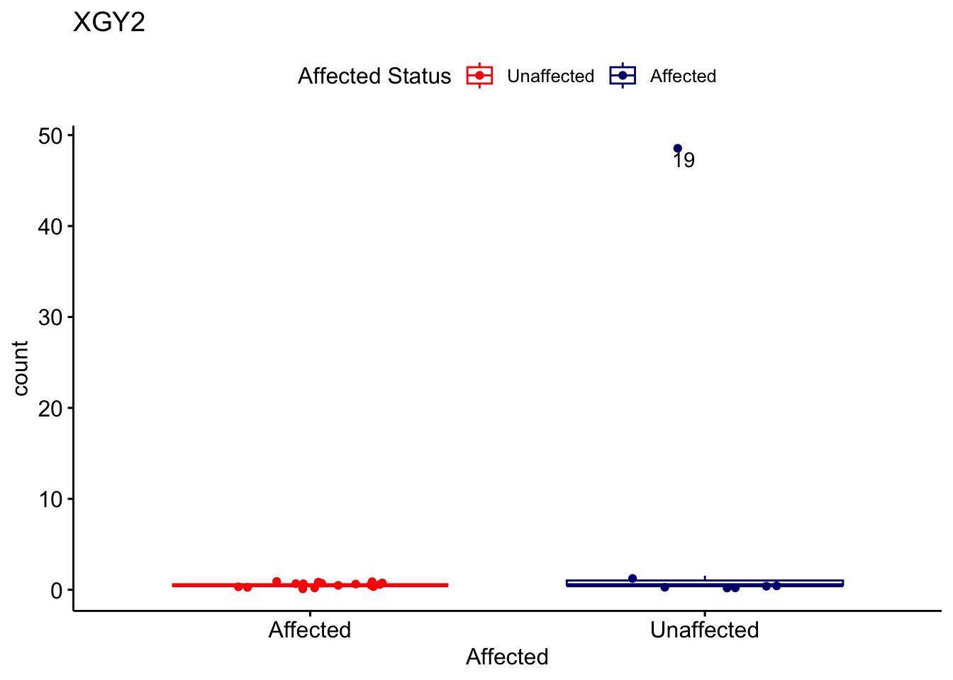
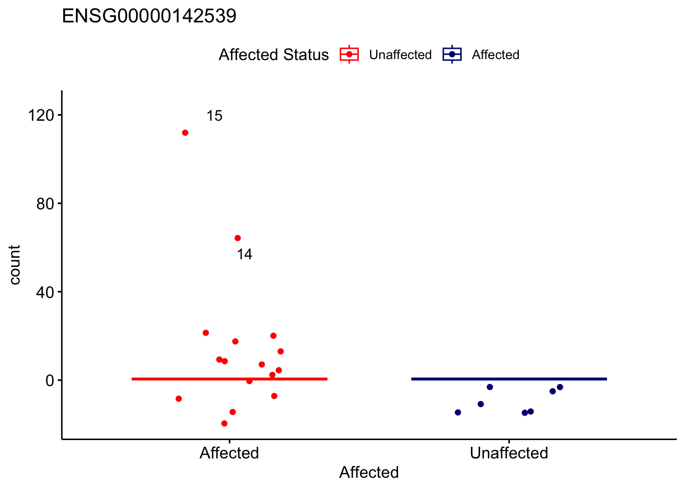
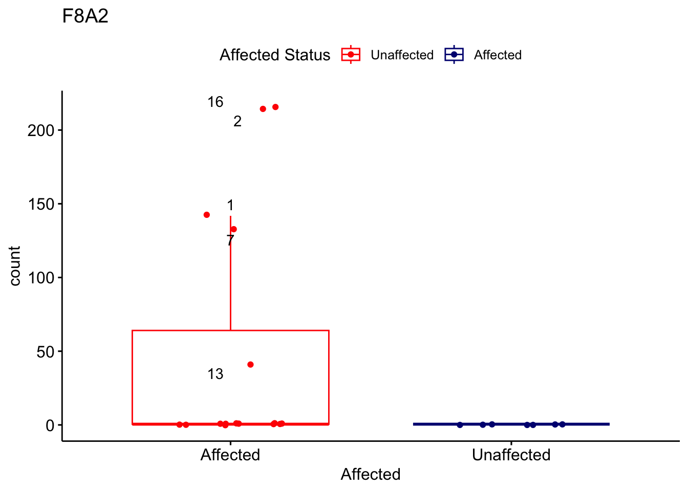
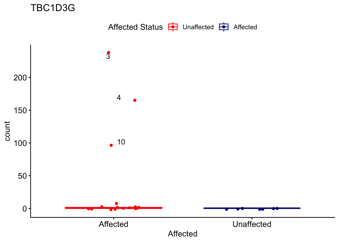
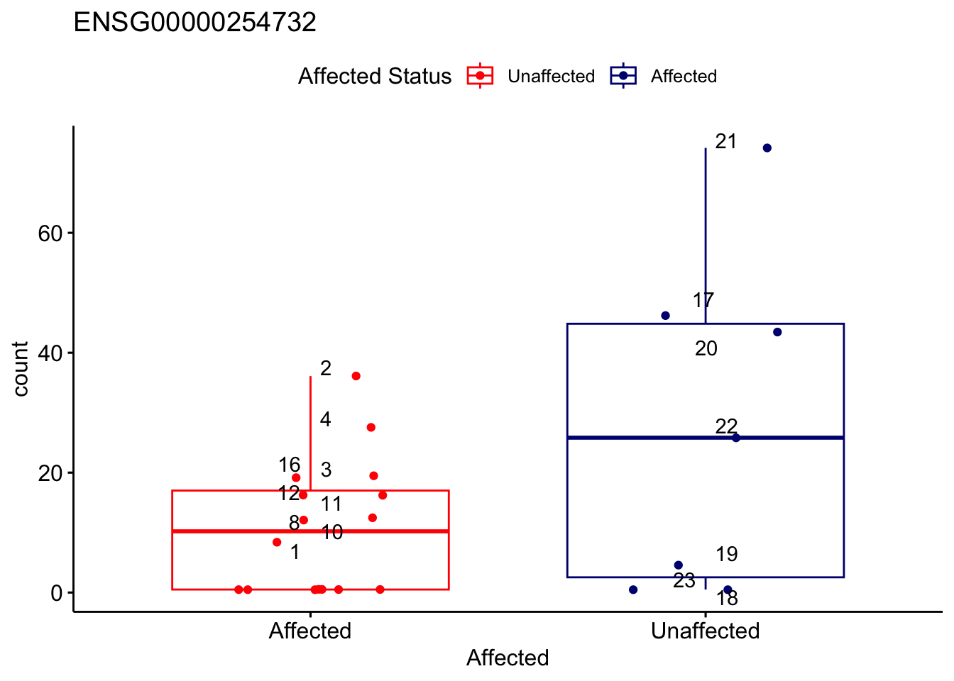
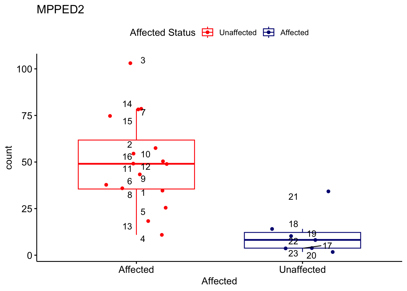
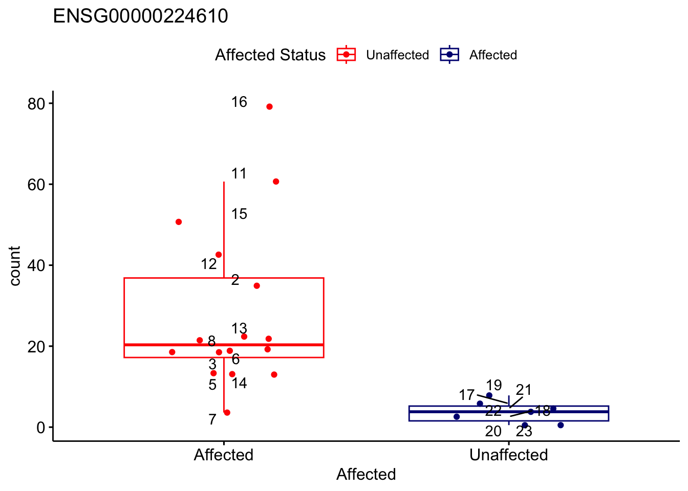
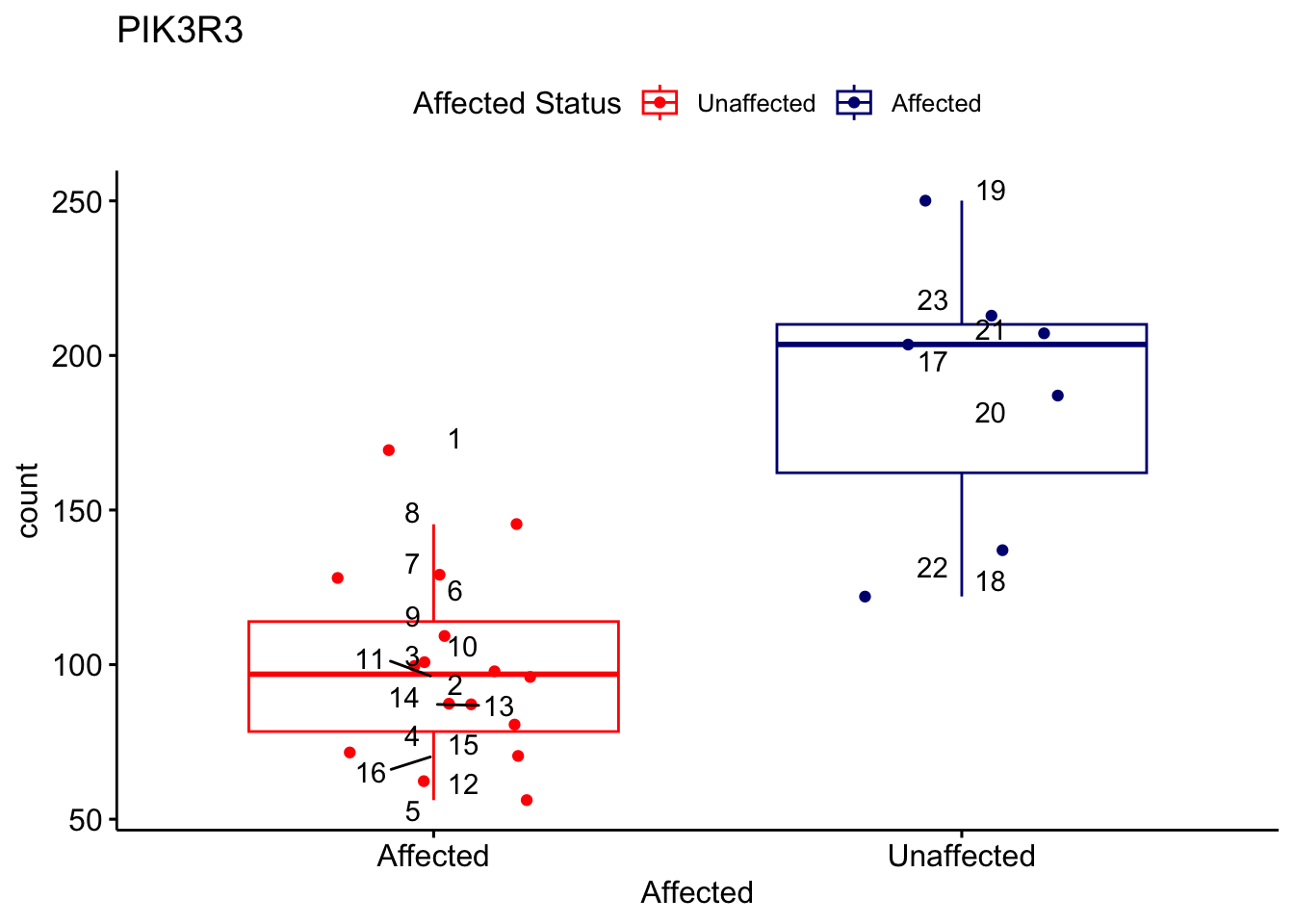
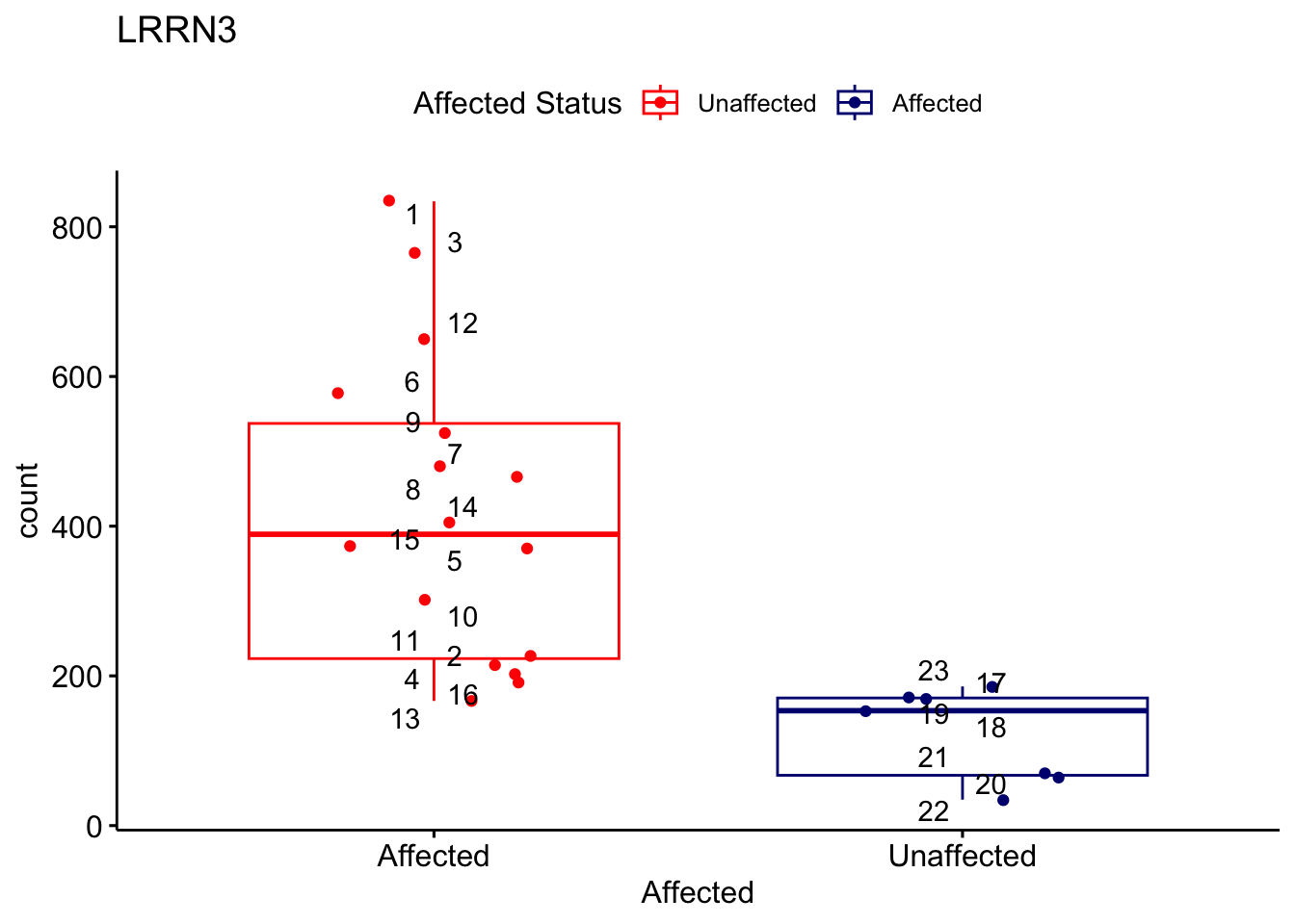
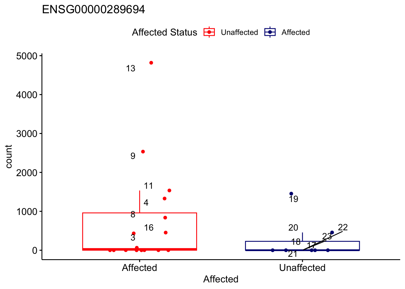
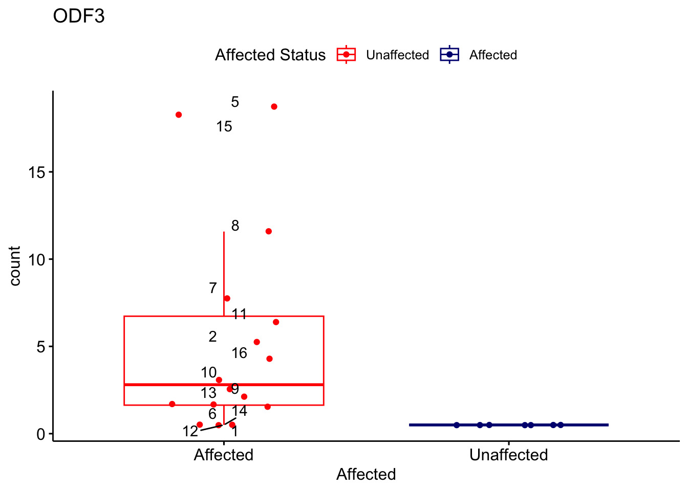
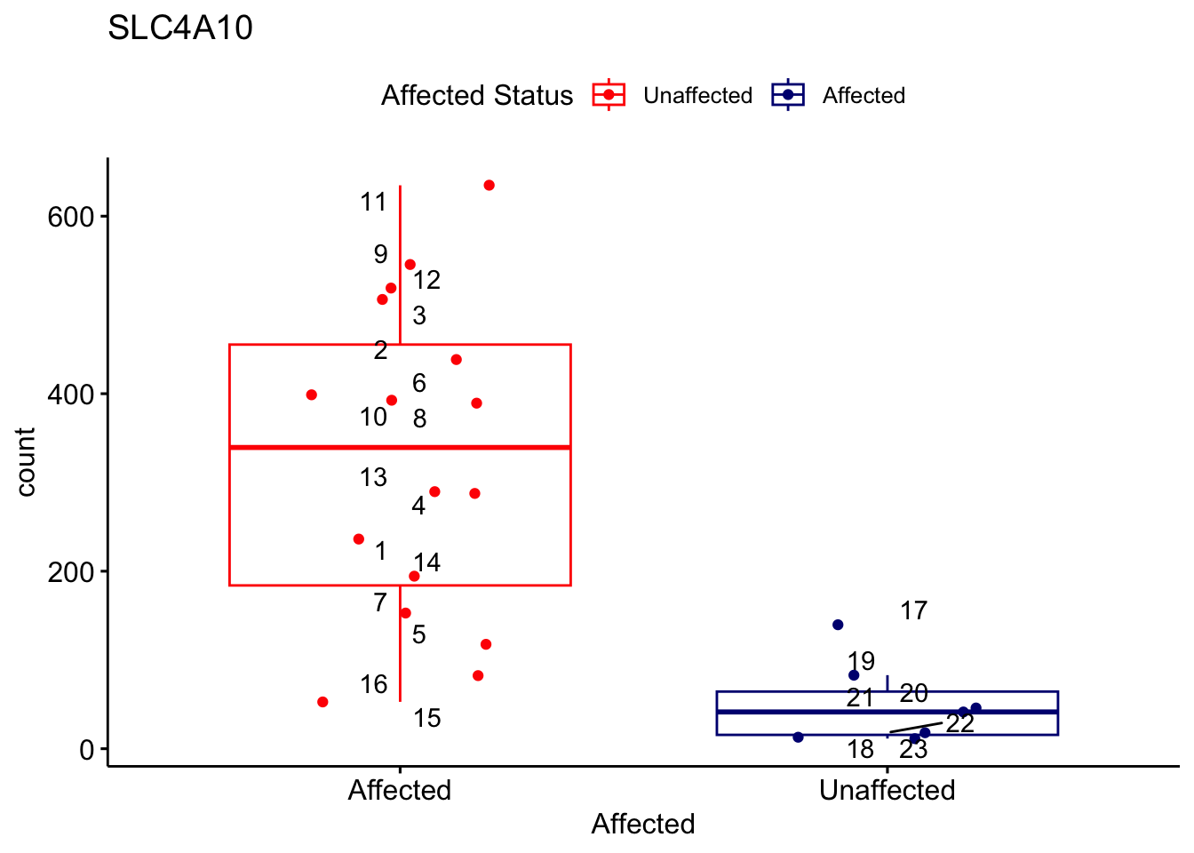
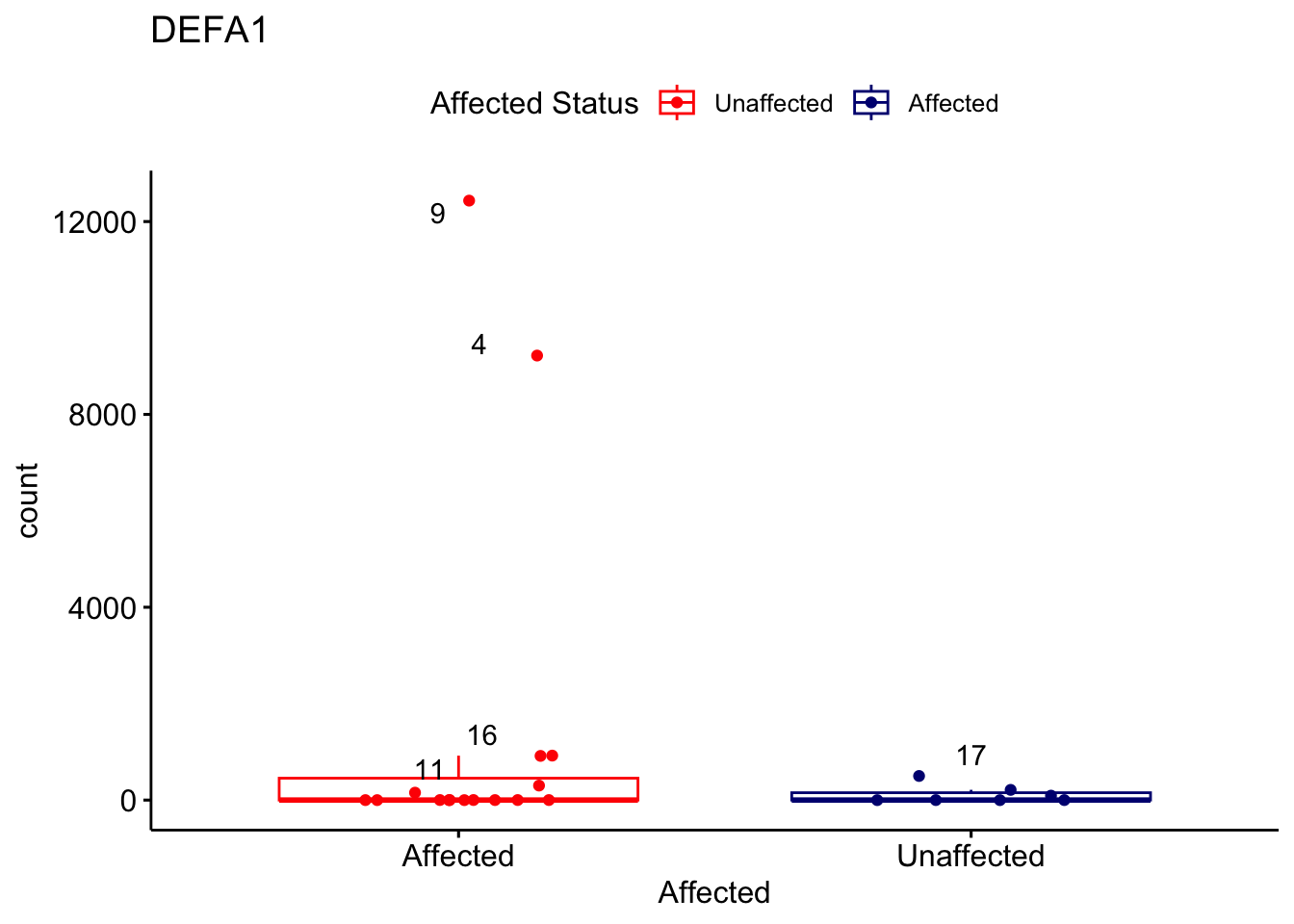
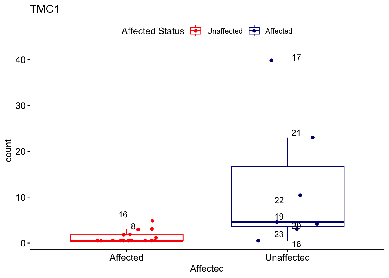
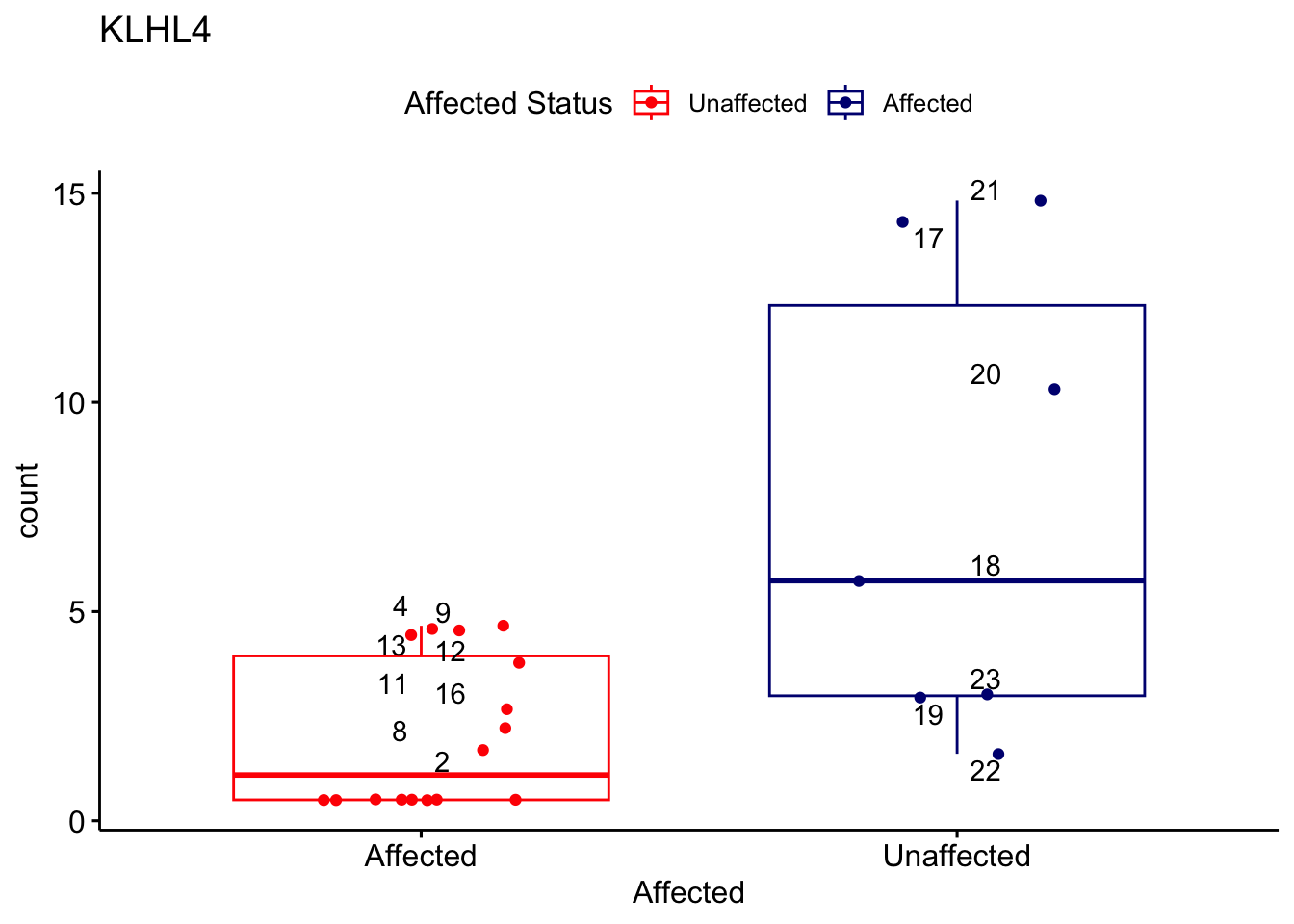
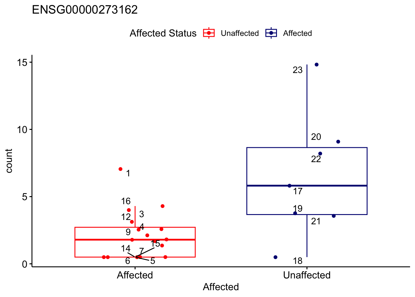
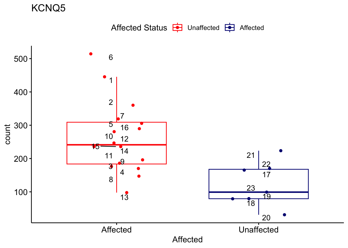
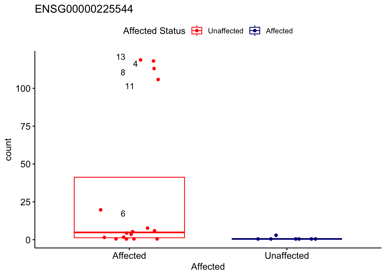
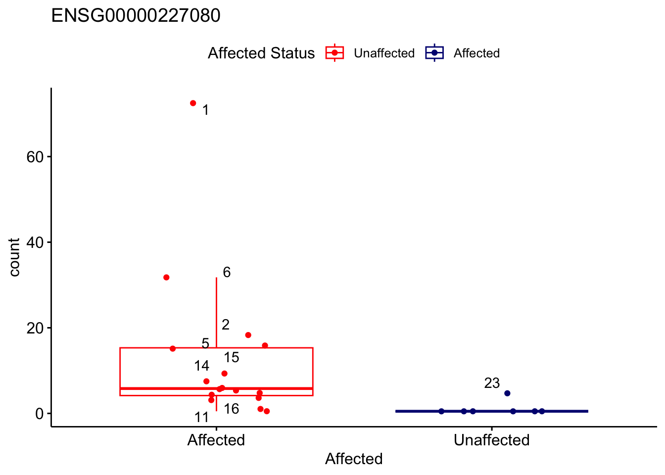
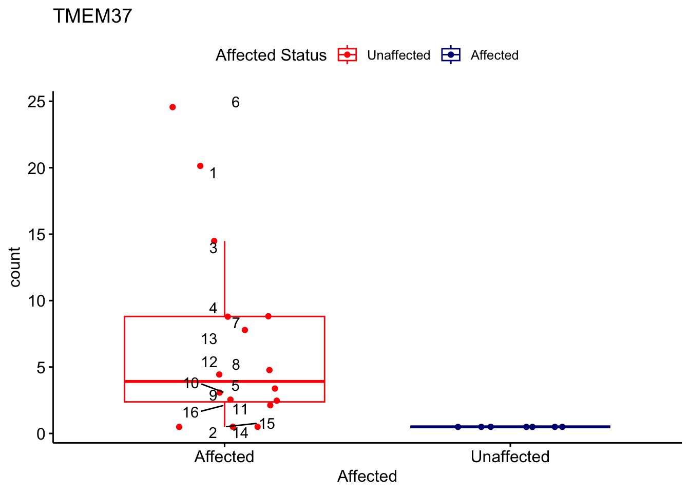
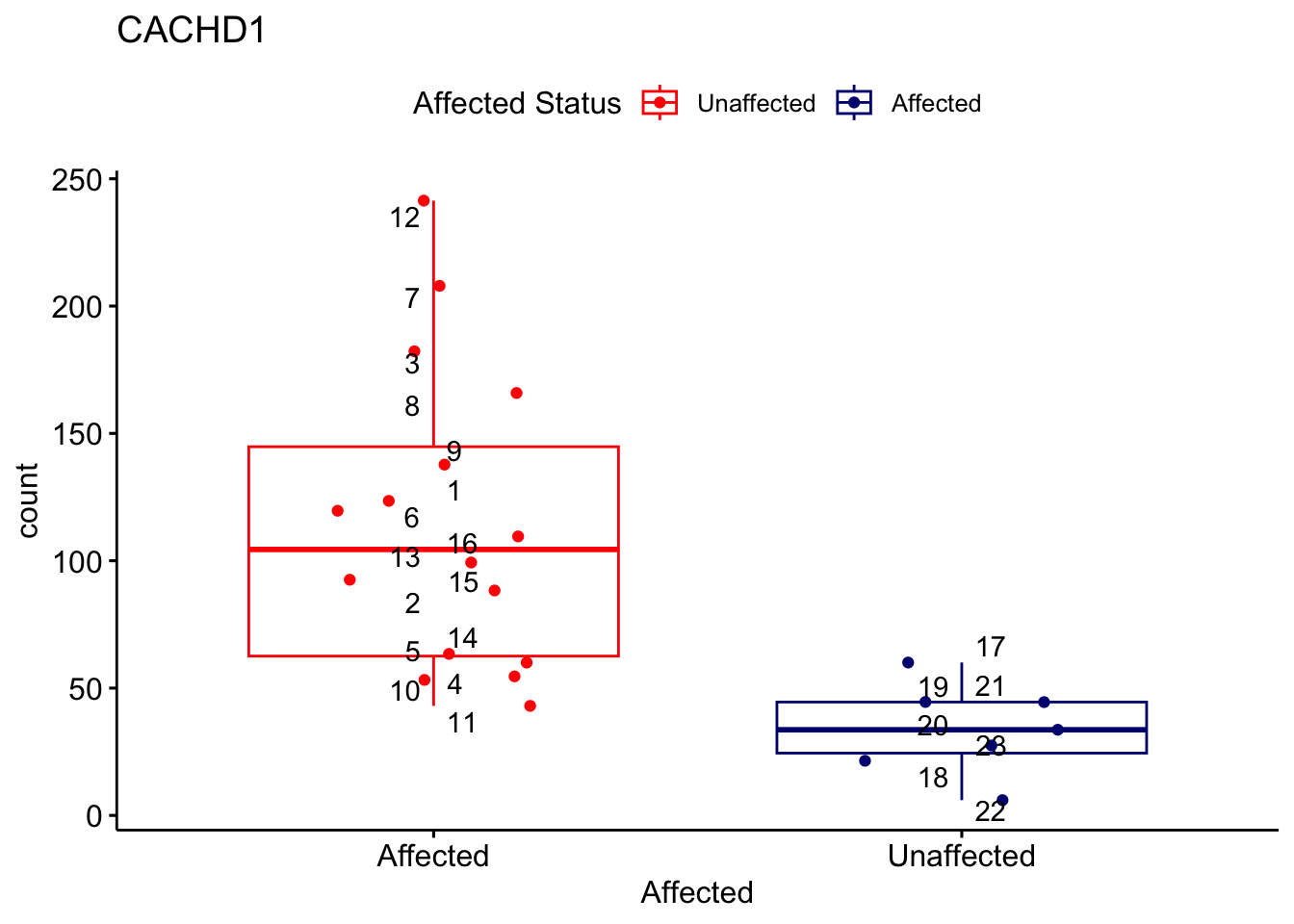
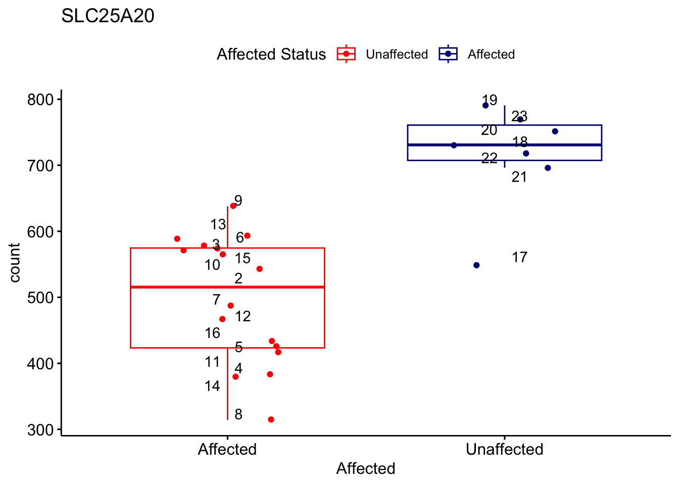
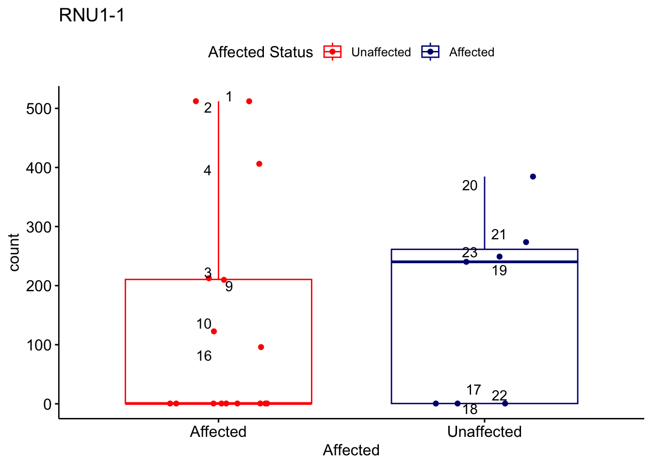
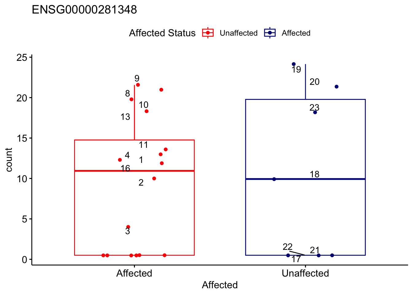
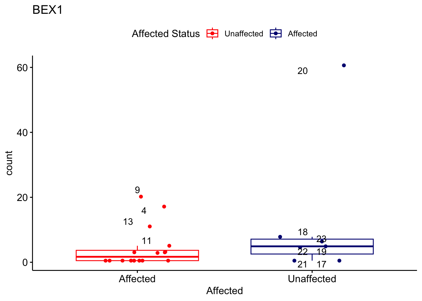
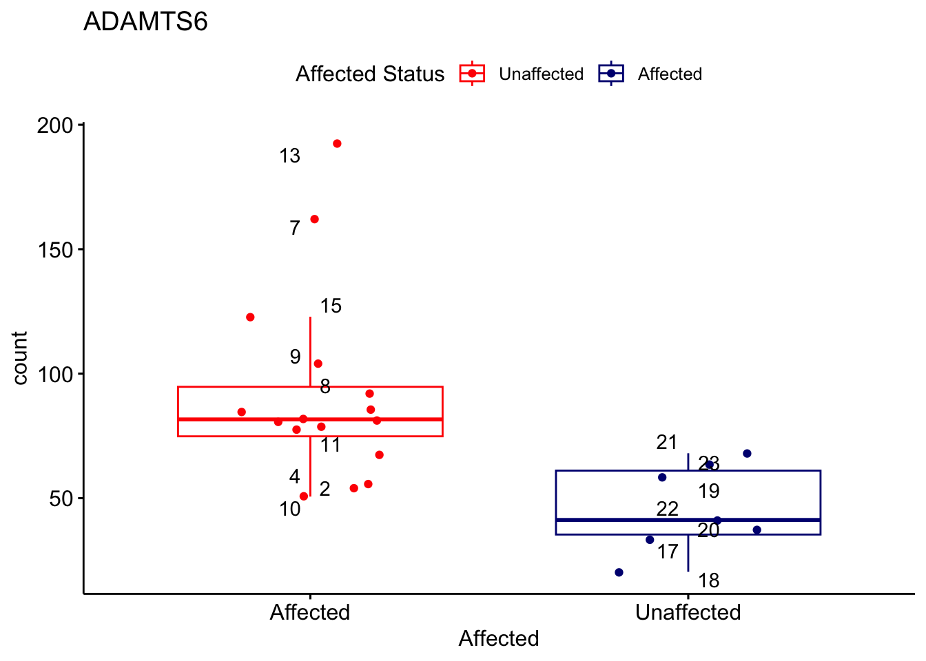
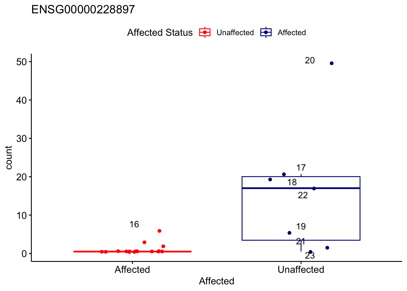
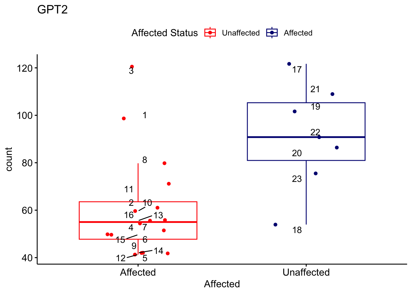
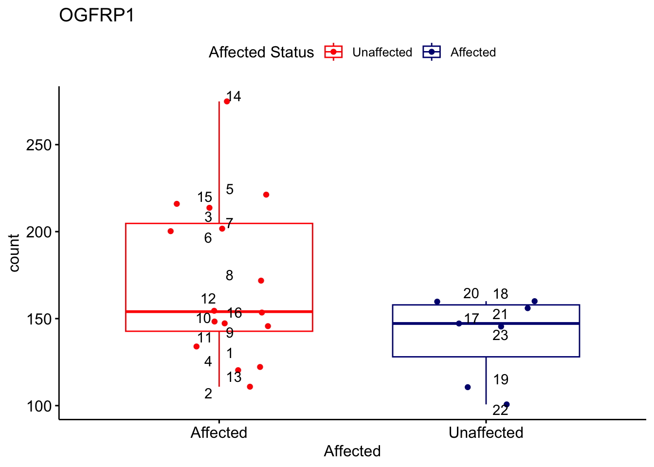
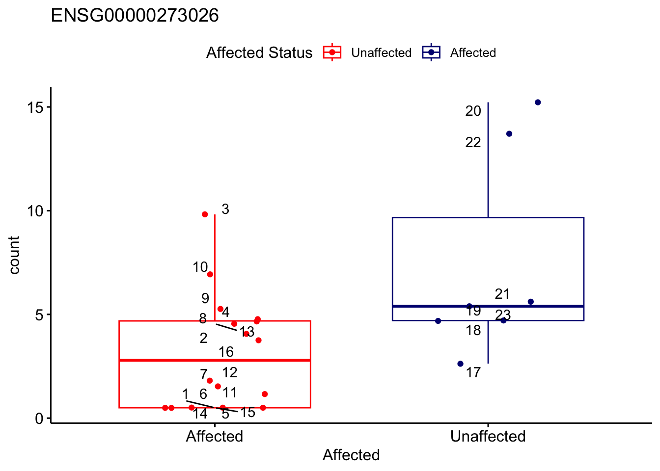
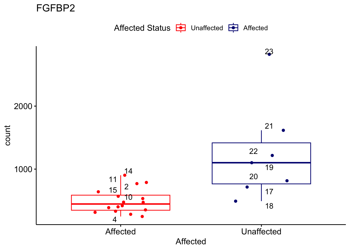
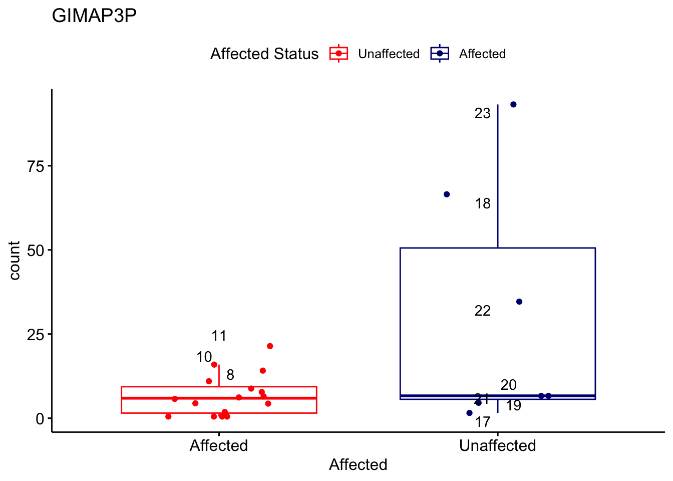
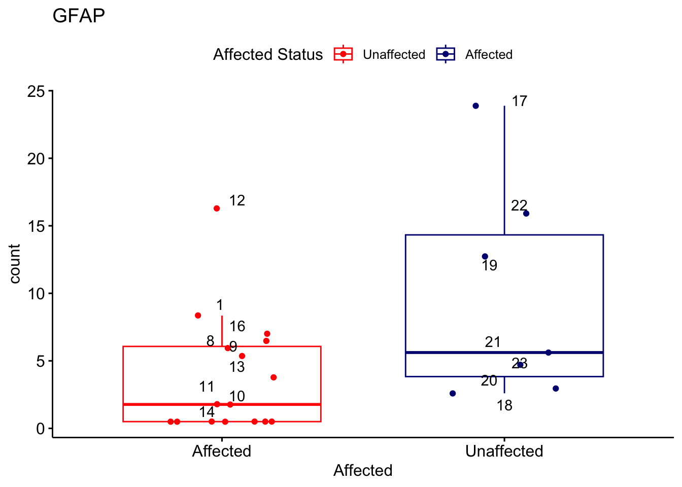
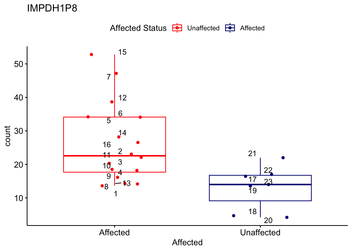
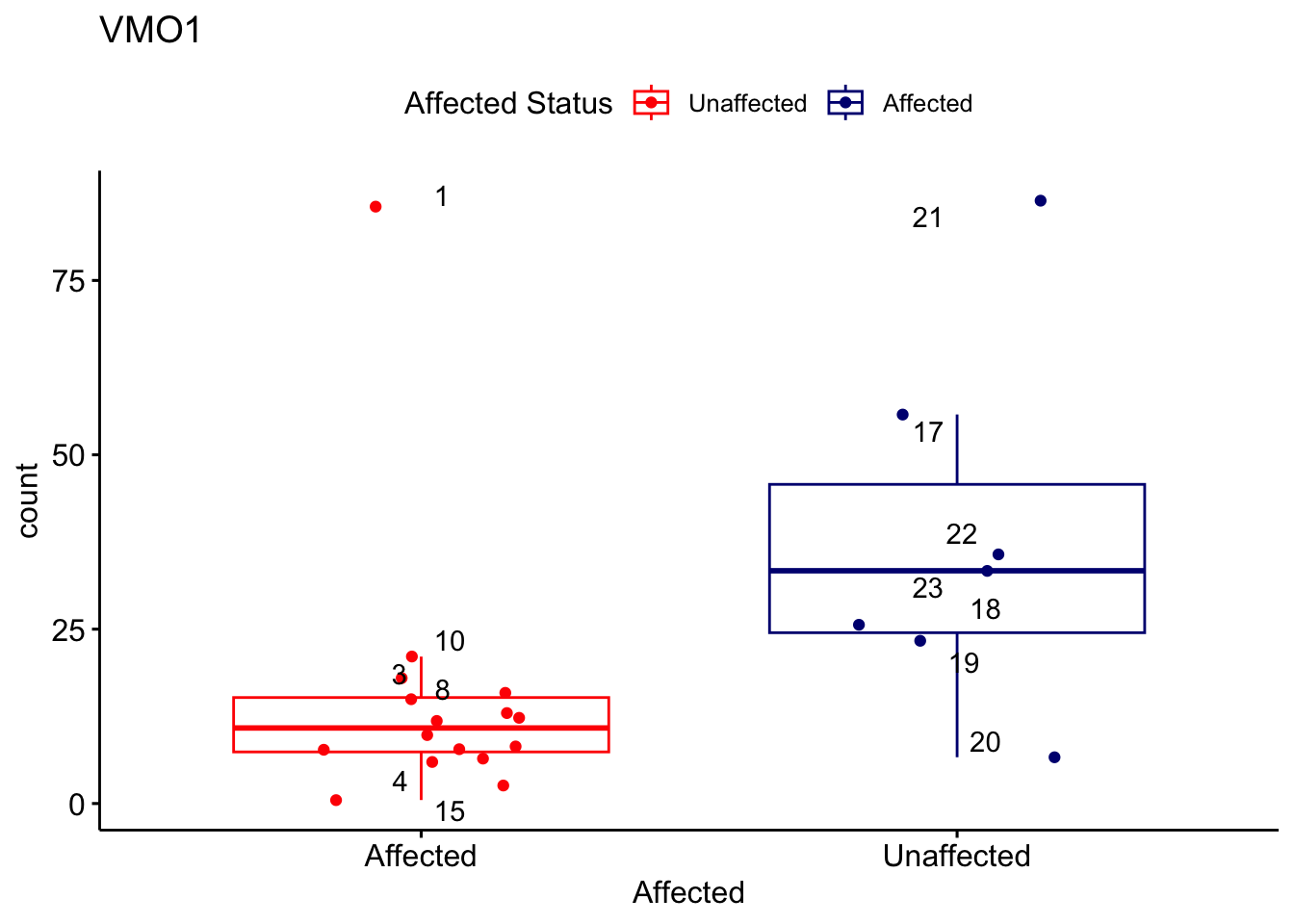
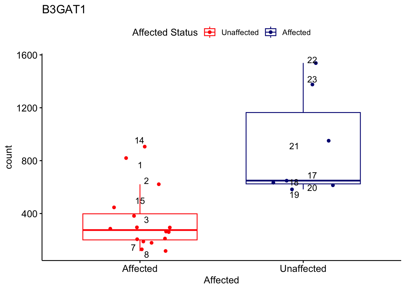
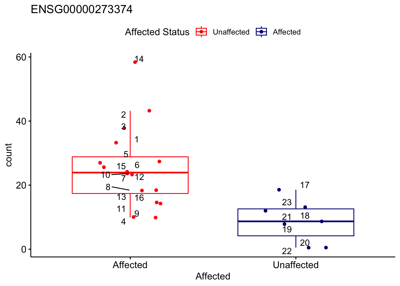
Genes of Interest Plot Counts
# Create an empty list to store the results for each gene
gene_results_list <- list()

# Loop through each gene to calculate and plot counts
for (ensembl_id in filtered_by_interest$Ensembl_ID) {
  d <- plotCounts(dds, gene = ensembl_id, intgroup = "Affected", returnData = TRUE)
  gene_name <- filtered_by_interest$gene_name[filtered_by_interest$Ensembl_ID == ensembl_id]

  # Calculate the mean and standard deviation of counts within each condition
  d_stats <- d %>%
    group_by(Affected) %>%
    summarise(
      mean_count = mean(count),
      sd_count = sd(count)
    )

  # Merge statistics back with the data
  d <- merge(d, d_stats, by = "Affected")

  # Create a temporary dataframe to store results for this gene
  temp_gene_df <- data.frame(
    Patient = rownames(d),
    stringsAsFactors = FALSE
  )

  # Calculate Z-scores and determine regulation status
  regulation_status <- sapply(1:nrow(d), function(i) {
    z_score <- (d$count[i] - d$mean_count[i]) / d$sd_count[i]

    # Determine regulation status based on Z-score
    if (z_score > 1) {
      return("Upregulated")
    } else if (z_score < -1) {
      return("Downregulated")
    } else {
      return("Neutral")
    }
  })

  # Add the regulation status to the temporary dataframe
  temp_gene_df[[gene_name]] <- regulation_status

  # Merge the temporary dataframe with the results list
  if (length(gene_results_list) == 0) {
    gene_results_list[[1]] <- temp_gene_df
  } else {
    gene_results_list[[1]] <- merge(gene_results_list[[1]], temp_gene_df, by = "Patient", all = TRUE)
  }

  # Generate the boxplot
  gene_plot <- ggboxplot(d,
    x = "Affected", y = "count", add = "jitter",
    color = "Affected", palette = c("red", "navy"),
    title = gene_name
  ) +
    geom_text_repel(aes(label = rownames(d))) +
    scale_color_manual(
      name = "Affected Status",
      labels = c("Unaffected", "Affected"),
      values = c("red", "navy")
    )
  print(gene_plot) # Ensure each plot is printed during the loop
  ggsave(
    filename = paste0(gene_name, "-subsetted-plot-counts.png"),
    path = "output/batch-correction-limma/plot-counts",
    plot = gene_plot, dpi = 450
  )
}
# Convert the list to a dataframe
gene_results_df <- gene_results_list[[1]]
file_name <- "output/genes_of_interest_plot_counts_signals.csv"
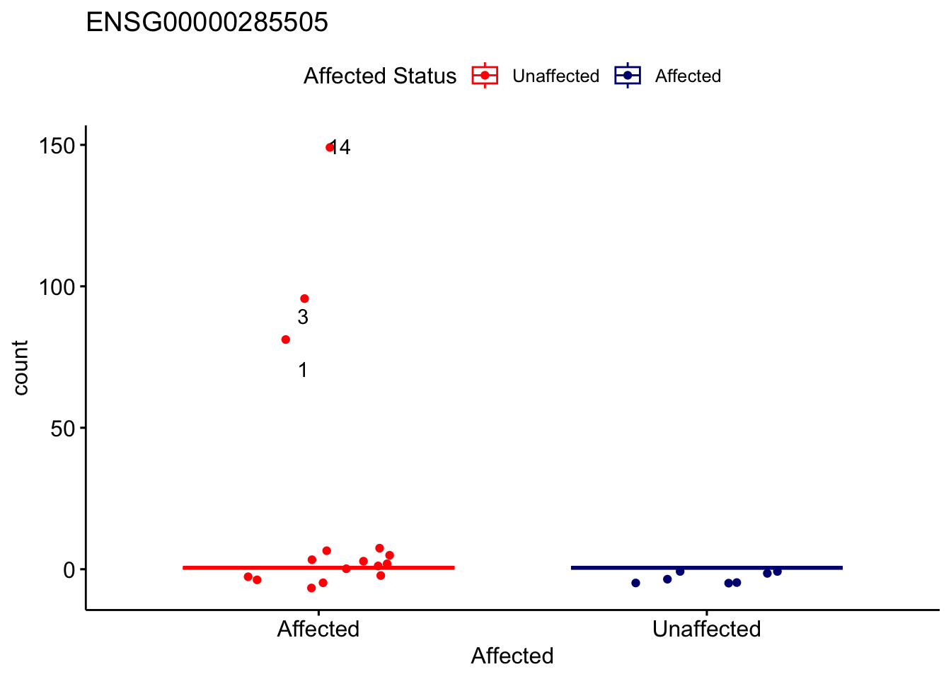
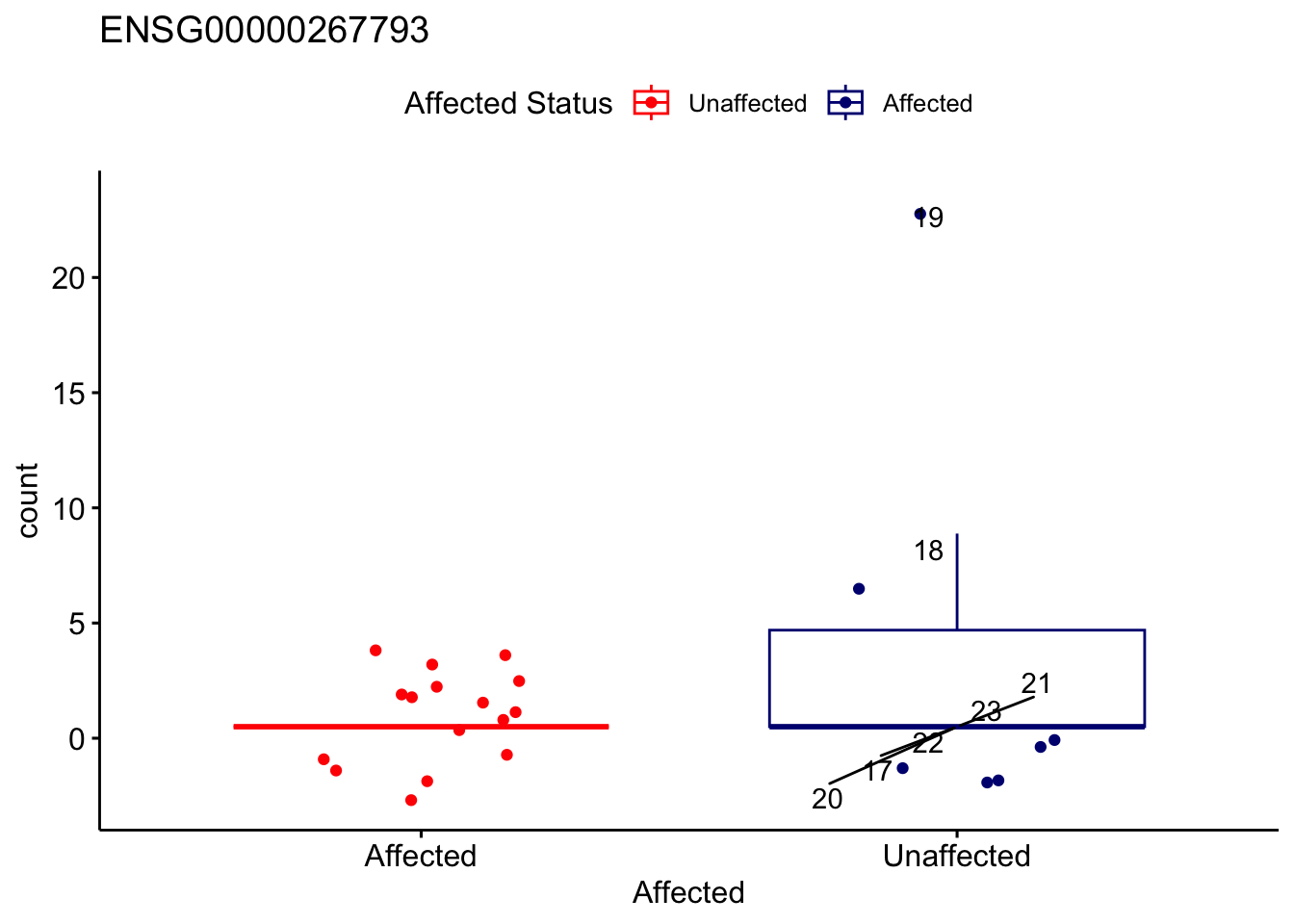
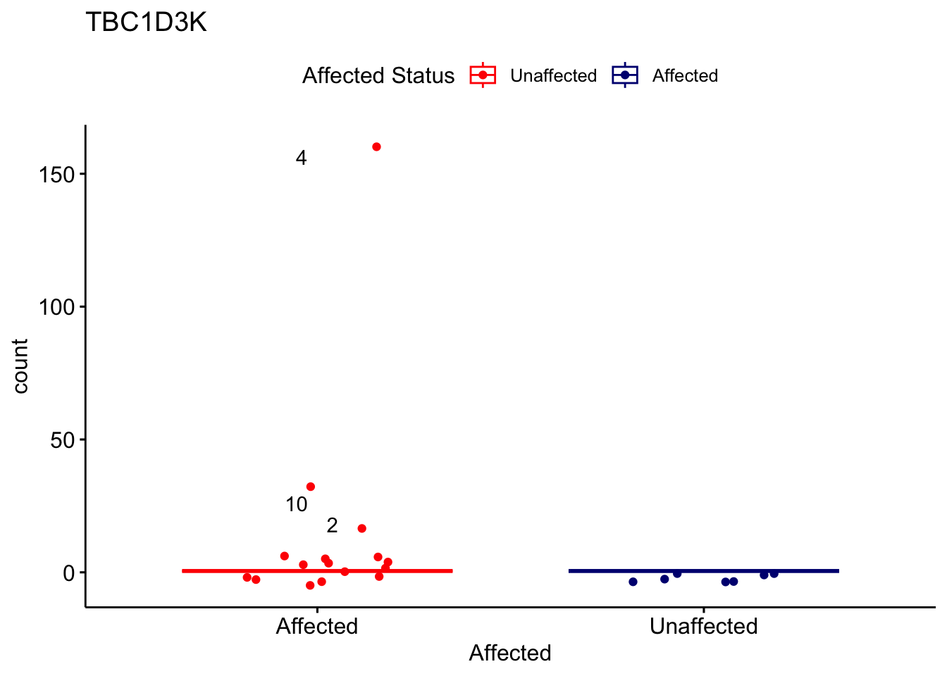
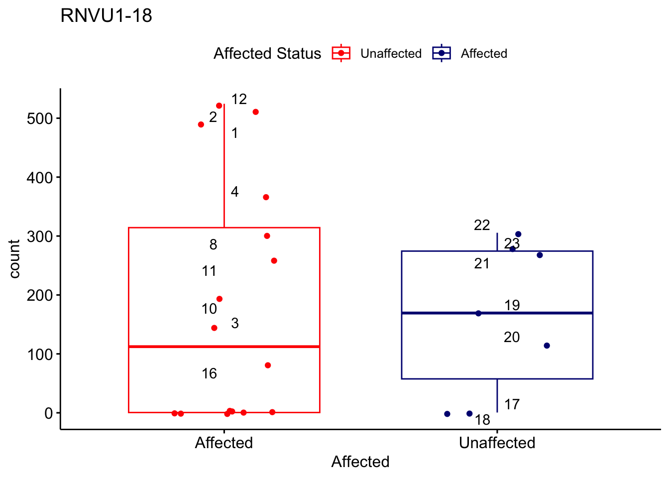
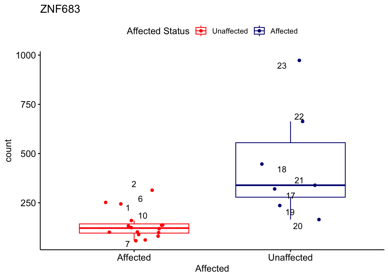
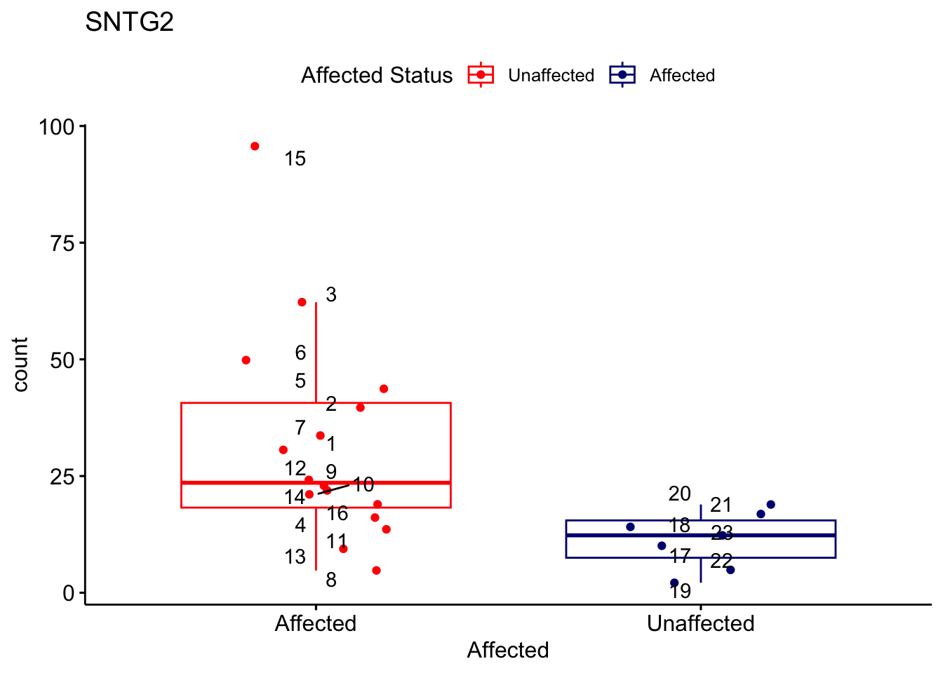
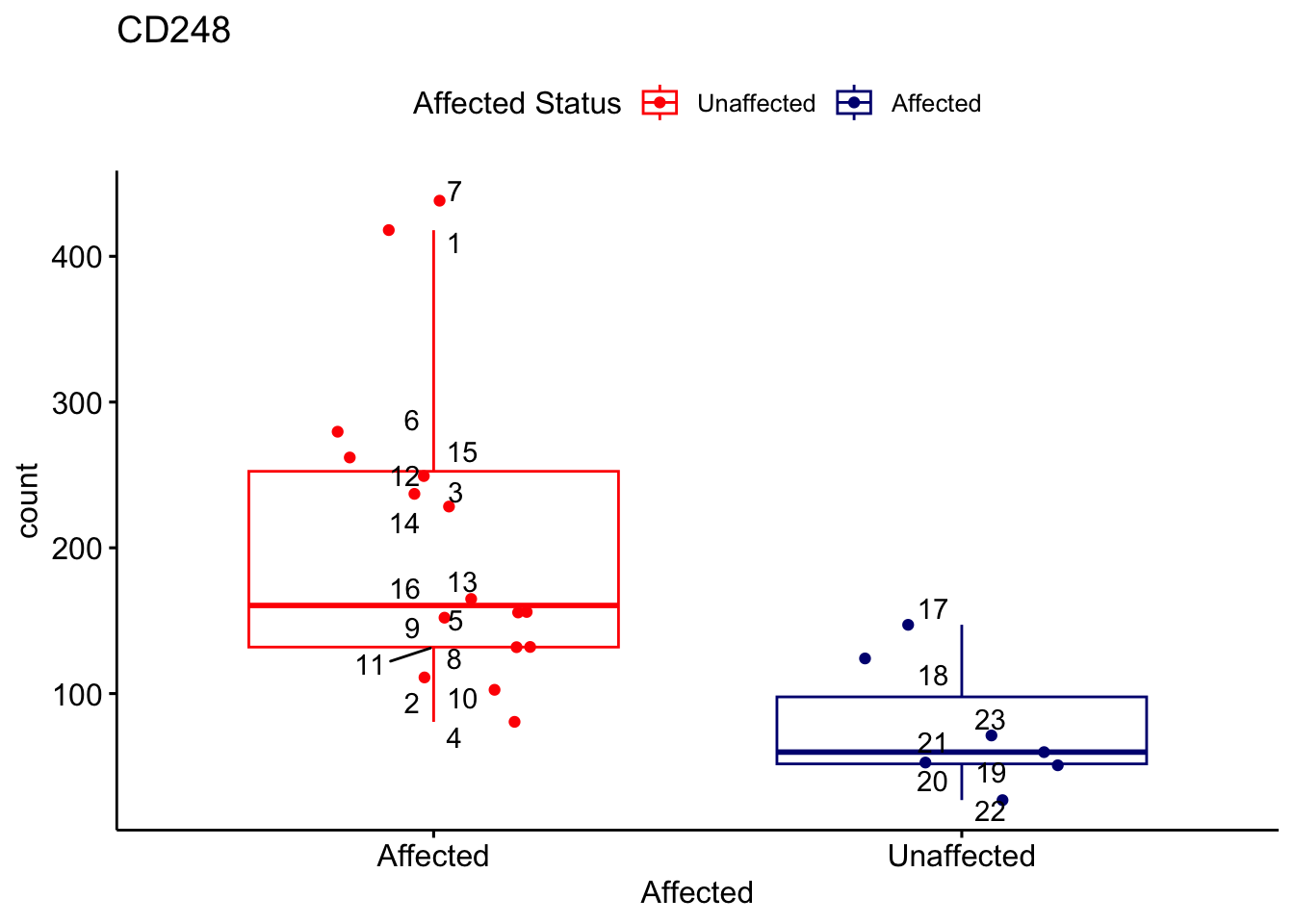
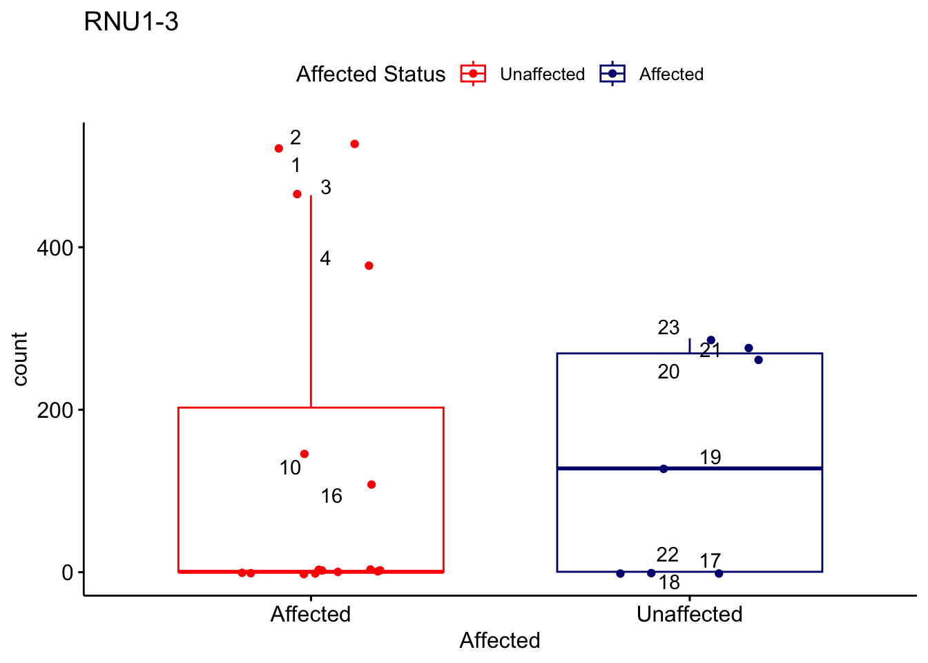
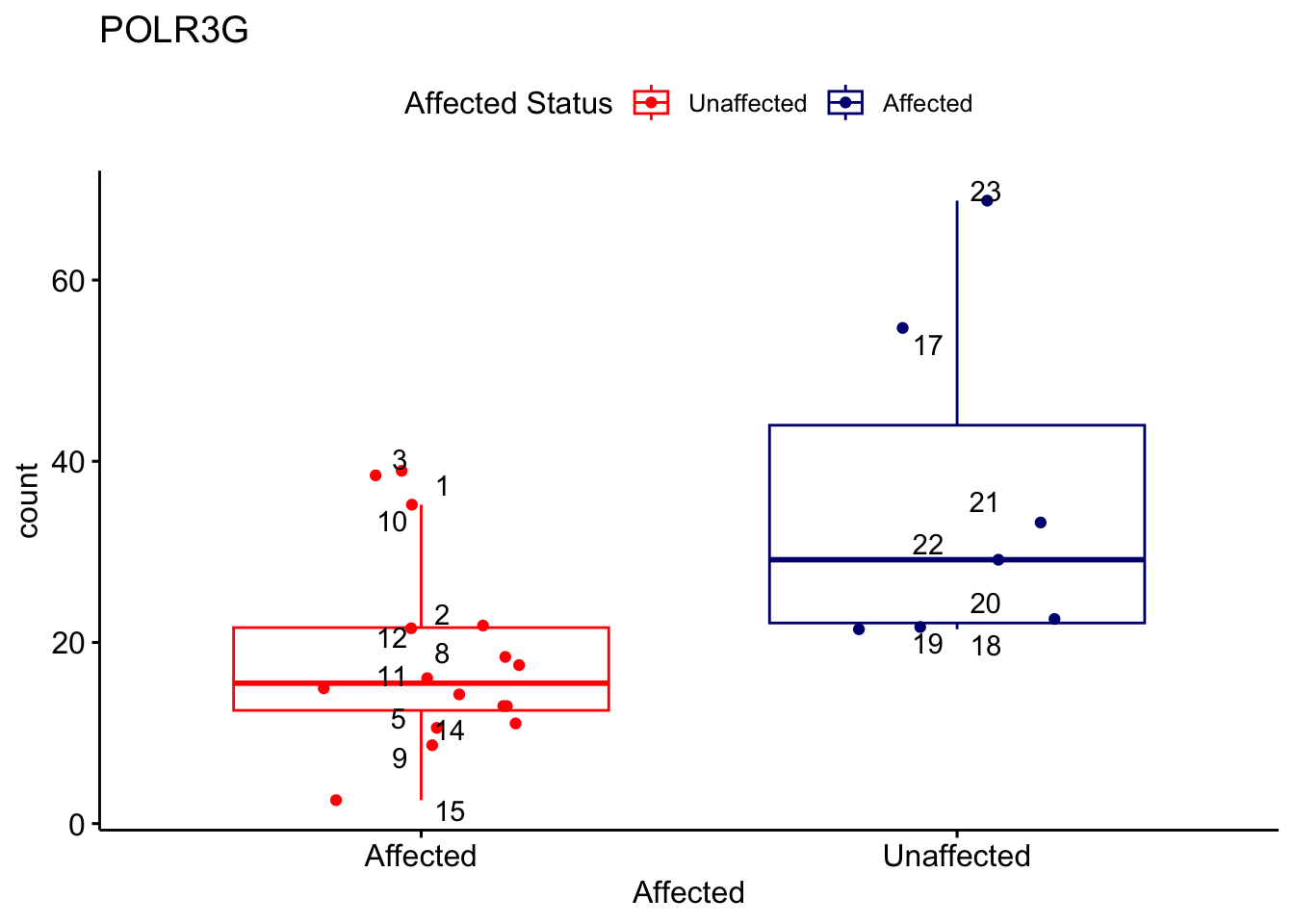
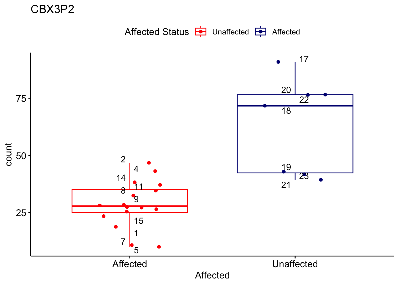
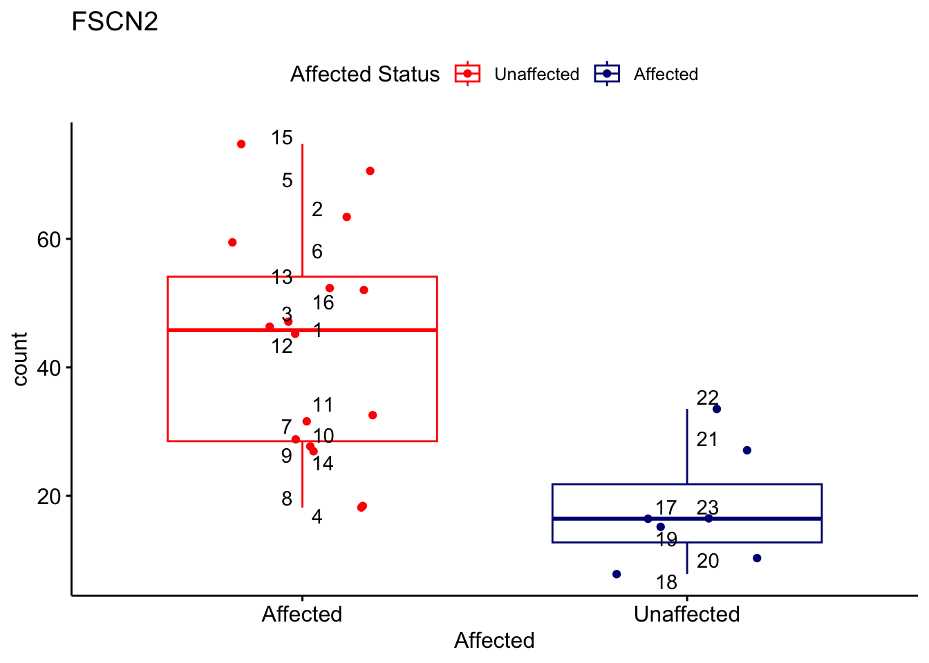
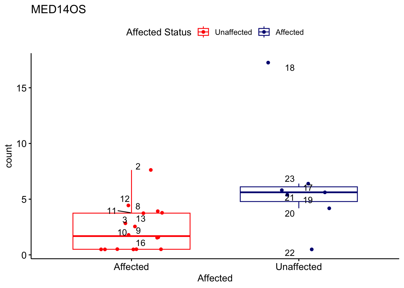
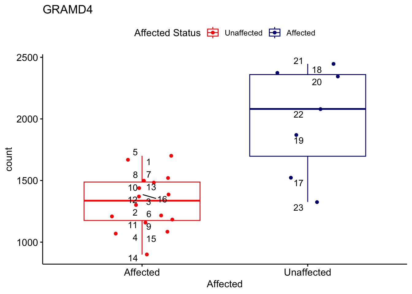
write.csv(gene_results_df, file_name, row.names = FALSE)Significant Genes Plot Counts
# Create an empty list to store the results for each gene
results_list <- list()

# Loop through each gene to calculate and plot counts
for (ensembl_id in res_aff_vs_unaff_df_genename_1$Ensembl_ID) {
  d <- plotCounts(dds, gene = ensembl_id, intgroup = "Affected", returnData = TRUE)
  gene_name <- res_aff_vs_unaff_df_genename_1$gene_name[res_aff_vs_unaff_df_genename_1$Ensembl_ID == ensembl_id]

  # Calculate the mean and standard deviation of counts within each condition
  d_stats <- d %>%
    group_by(Affected) %>%
    summarise(
      mean_count = mean(count),
      sd_count = sd(count)
    )

  # Merge statistics back with the data
  d <- merge(d, d_stats, by = "Affected")

  # Create a temporary dataframe to store results for this gene
  temp_df <- data.frame(
    Patient = rownames(d),
    stringsAsFactors = FALSE
  )

  # Calculate Z-scores and determine regulation status
  regulation_status <- sapply(1:nrow(d), function(i) {
    if (is.na(d$sd_count[i]) || d$sd_count[i] == 0) {
      return("Neutral")
    }

    z_score <- (d$count[i] - d$mean_count[i]) / d$sd_count[i]

    # Determine regulation status based on Z-score
    if (is.na(z_score)) {
      return("Neutral")
    } else if (z_score > 1) {
      return("Upregulated")
    } else if (z_score < -1) {
      return("Downregulated")
    } else {
      return("Neutral")
    }
  })

  # Add the regulation status to the temporary dataframe
  temp_df[[gene_name]] <- regulation_status

  # Merge the temporary dataframe with the results list
  if (length(results_list) == 0) {
    results_list[[1]] <- temp_df
  } else {
    results_list[[1]] <- merge(results_list[[1]], temp_df, by = "Patient", all = TRUE)
  }

  # Generate the boxplot
  ggplot_box <- ggboxplot(d,
    x = "Affected", y = "count", add = "jitter",
    color = "Affected", palette = c("red", "navy"),
    title = gene_name
  ) +
    geom_text_repel(aes(label = rownames(d))) +
    scale_color_manual(
      name = "Affected Status",
      labels = c("Unaffected", "Affected"),
      values = c("red", "navy")
    )
  print(ggplot_box) # Ensure each plot is printed during the loop
  ggsave(
    filename = paste0(gene_name, "-subsetted-plot-counts.png"),
    path = "output/batch-correction-limma/plot-counts",
    plot = ggplot_box, dpi = 450
  )
}
# Convert the list to a dataframe
results_df <- results_list[[1]]

file_name <- "output/significant_plot_counts_signals.csv"
write.csv(results_df, file_name, row.names = FALSE)
Combined Heatmap of DEGs and Patient Genes
mat3 <- assay(vsd_limma)[filtered_by_interest$Ensembl_ID, ]
rownames(mat3) <- gene_info$gene_name[match(filtered_by_interest$Ensembl_ID, gene_info$Ensembl_ID)]
df_sub <- as.data.frame(colData(vsd_limma)[, c("Affected", "Category")])
pheatmap(mat3, annotation_col = df_sub, annotation_colors = ann_colors2, fontsize = 4, angle_col = 0)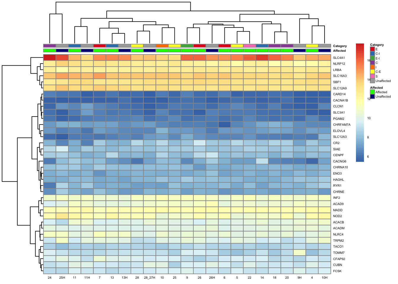
Save data
save.image(file = "output/subsetted-condition-analysis.RData")
sessionInfo()R version 4.4.0 (2024-04-24)
Platform: x86_64-apple-darwin20
Running under: macOS Sonoma 14.5
Matrix products: default
BLAS: /Library/Frameworks/R.framework/Versions/4.4-x86_64/Resources/lib/libRblas.0.dylib
LAPACK: /Library/Frameworks/R.framework/Versions/4.4-x86_64/Resources/lib/libRlapack.dylib; LAPACK version 3.12.0
locale:
[1] en_US.UTF-8/en_US.UTF-8/en_US.UTF-8/C/en_US.UTF-8/en_US.UTF-8
time zone: America/Chicago
tzcode source: internal
attached base packages:
[1] stats4 stats graphics grDevices datasets utils methods
[8] base
other attached packages:
[1] STRINGdb_2.16.4 enrichR_3.2
[3] DOSE_3.30.1 mygene_1.40.0
[5] txdbmaker_1.0.0 GenomicFeatures_1.56.0
[7] ReactomePA_1.48.0 ggrepel_0.9.5
[9] org.Hs.eg.db_3.19.1 AnnotationDbi_1.66.0
[11] clusterProfiler_4.12.0 rmarkdown_2.27
[13] ggpubr_0.6.0 plotly_4.10.4
[15] biomaRt_2.60.0 gprofiler2_0.2.3
[17] limma_3.60.2 genefilter_1.86.0
[19] pheatmap_1.0.12 RColorBrewer_1.1-3
[21] DESeq2_1.44.0 SummarizedExperiment_1.34.0
[23] Biobase_2.64.0 MatrixGenerics_1.16.0
[25] matrixStats_1.3.0 GenomicRanges_1.56.0
[27] GenomeInfoDb_1.40.1 IRanges_2.38.0
[29] S4Vectors_0.42.0 BiocGenerics_0.50.0
[31] lubridate_1.9.3 forcats_1.0.0
[33] stringr_1.5.1 dplyr_1.1.4
[35] purrr_1.0.2 readr_2.1.5
[37] tidyr_1.3.1 tibble_3.2.1
[39] ggplot2_3.5.1 tidyverse_2.0.0
[41] workflowr_1.7.1
loaded via a namespace (and not attached):
[1] fs_1.6.4 bitops_1.0-7 enrichplot_1.24.0
[4] doParallel_1.0.17 HDO.db_0.99.1 httr_1.4.7
[7] tools_4.4.0 backports_1.5.0 utf8_1.2.4
[10] R6_2.5.1 lazyeval_0.2.2 GetoptLong_1.0.5
[13] withr_3.0.0 graphite_1.50.0 prettyunits_1.2.0
[16] gridExtra_2.3 textshaping_0.4.0 cli_3.6.2
[19] scatterpie_0.2.3 labeling_0.4.3 sass_0.4.9
[22] systemfonts_1.1.0 Rsamtools_2.20.0 yulab.utils_0.1.4
[25] gson_0.1.0 foreign_0.8-86 WriteXLS_6.6.0
[28] plotrix_3.8-4 rstudioapi_0.16.0 RSQLite_2.3.7
[31] shape_1.4.6.1 generics_0.1.3 gridGraphics_0.5-1
[34] BiocIO_1.14.0 vroom_1.6.5 gtools_3.9.5
[37] car_3.1-2 GO.db_3.19.1 Matrix_1.7-0
[40] fansi_1.0.6 abind_1.4-5 lifecycle_1.0.4
[43] whisker_0.4.1 yaml_2.3.8 carData_3.0-5
[46] gplots_3.1.3.1 qvalue_2.36.0 SparseArray_1.4.8
[49] BiocFileCache_2.12.0 grid_4.4.0 blob_1.2.4
[52] promises_1.3.0 crayon_1.5.2 lattice_0.22-6
[55] cowplot_1.1.3 annotate_1.82.0 KEGGREST_1.44.0
[58] ComplexHeatmap_2.16.0 pillar_1.9.0 knitr_1.47
[61] fgsea_1.30.0 rjson_0.2.21 codetools_0.2-20
[64] fastmatch_1.1-4 glue_1.7.0 getPass_0.2-4
[67] ggfun_0.1.5 data.table_1.15.4 vctrs_0.6.5
[70] png_0.1-8 treeio_1.28.0 gtable_0.3.5
[73] gsubfn_0.7 cachem_1.1.0 xfun_0.44
[76] S4Arrays_1.4.1 tidygraph_1.3.1 survival_3.5-8
[79] iterators_1.0.14 statmod_1.5.0 nlme_3.1-164
[82] ggtree_3.12.0 bit64_4.0.5 progress_1.2.3
[85] filelock_1.0.3 rprojroot_2.0.4 bslib_0.7.0
[88] KernSmooth_2.23-22 rpart_4.1.23 colorspace_2.1-0
[91] DBI_1.2.3 Hmisc_5.1-3 nnet_7.3-19
[94] tidyselect_1.2.1 processx_3.8.4 chron_2.3-61
[97] bit_4.0.5 compiler_4.4.0 curl_5.2.1
[100] git2r_0.33.0 httr2_1.0.1 graph_1.82.0
[103] htmlTable_2.4.2 xml2_1.3.6 DelayedArray_0.30.1
[106] shadowtext_0.1.3 rtracklayer_1.64.0 caTools_1.18.2
[109] checkmate_2.3.1 scales_1.3.0 callr_3.7.6
[112] rappdirs_0.3.3 digest_0.6.35 XVector_0.44.0
[115] htmltools_0.5.8.1 pkgconfig_2.0.3 base64enc_0.1-3
[118] highr_0.11 dbplyr_2.5.0 fastmap_1.2.0
[121] GlobalOptions_0.1.2 ggthemes_5.1.0 rlang_1.1.4
[124] htmlwidgets_1.6.4 UCSC.utils_1.0.0 farver_2.1.2
[127] jquerylib_0.1.4 jsonlite_1.8.8 BiocParallel_1.38.0
[130] GOSemSim_2.30.0 RCurl_1.98-1.14 magrittr_2.0.3
[133] Formula_1.2-5 GenomeInfoDbData_1.2.12 ggplotify_0.1.2
[136] patchwork_1.2.0 munsell_0.5.1 Rcpp_1.0.12
[139] proto_1.0.0 ape_5.8 viridis_0.6.5
[142] sqldf_0.4-11 stringi_1.8.4 ggraph_2.2.1
[145] zlibbioc_1.50.0 MASS_7.3-60.2 plyr_1.8.9
[148] parallel_4.4.0 Biostrings_2.72.1 graphlayouts_1.1.1
[151] splines_4.4.0 hash_2.2.6.3 circlize_0.4.16
[154] hms_1.1.3 locfit_1.5-9.9 ps_1.7.6
[157] igraph_2.0.3 ggsignif_0.6.4 reshape2_1.4.4
[160] XML_3.99-0.16.1 evaluate_0.24.0 renv_1.0.7
[163] BiocManager_1.30.23 foreach_1.5.2 tzdb_0.4.0
[166] tweenr_2.0.3 httpuv_1.6.15 polyclip_1.10-6
[169] clue_0.3-65 ggforce_0.4.2 broom_1.0.6
[172] xtable_1.8-4 restfulr_0.0.15 reactome.db_1.88.0
[175] tidytree_0.4.6 rstatix_0.7.2 later_1.3.2
[178] ragg_1.3.2 viridisLite_0.4.2 aplot_0.2.2
[181] memoise_2.0.1 GenomicAlignments_1.40.0 cluster_2.1.6
[184] timechange_0.3.0