Differential Gene Expression (DGE) Analysis
Last updated: 2023-07-01
Checks: 7 0
Knit directory: mecfs-dge-analysis/
This reproducible R Markdown analysis was created with workflowr (version 1.7.0). The Checks tab describes the reproducibility checks that were applied when the results were created. The Past versions tab lists the development history.
Great! Since the R Markdown file has been committed to the Git repository, you know the exact version of the code that produced these results.
Great job! The global environment was empty. Objects defined in the global environment can affect the analysis in your R Markdown file in unknown ways. For reproduciblity it’s best to always run the code in an empty environment.
The command set.seed(20230618) was run prior to running
the code in the R Markdown file. Setting a seed ensures that any results
that rely on randomness, e.g. subsampling or permutations, are
reproducible.
Great job! Recording the operating system, R version, and package versions is critical for reproducibility.
Nice! There were no cached chunks for this analysis, so you can be confident that you successfully produced the results during this run.
Great job! Using relative paths to the files within your workflowr project makes it easier to run your code on other machines.
Great! You are using Git for version control. Tracking code development and connecting the code version to the results is critical for reproducibility.
The results in this page were generated with repository version b5cecfb. See the Past versions tab to see a history of the changes made to the R Markdown and HTML files.
Note that you need to be careful to ensure that all relevant files for
the analysis have been committed to Git prior to generating the results
(you can use wflow_publish or
wflow_git_commit). workflowr only checks the R Markdown
file, but you know if there are other scripts or data files that it
depends on. Below is the status of the Git repository when the results
were generated:
Ignored files:
    Ignored:    .DS_Store
    Ignored:    .Rhistory
    Ignored:    .Rproj.user/
    Ignored:    data/.DS_Store
    Ignored:    output/batch-correction-limma/

Untracked files:
    Untracked:  data/MECFS_RNAseq_metadata_2023_06_23.csv
    Untracked:  data/RNAseq Variants of Interest List_V2.xlsx

Unstaged changes:
    Deleted:    Rplot.png
    Modified:   code/helpers.R
    Deleted:    data/CPAM0066_PCS_slides_NM_001173543.1(BANP) c.1372G-A, p.Val458Met.pptx
    Deleted:    data/MECFS_RNAseq_metadata_CORRECTED.csv
    Deleted:    data/MECFS_RNAseq_metadata_CORRECTED.xlsx
    Modified:   output/counts_vst.csv
    Modified:   output/counts_vst_limma.csv
    Modified:   output/res_aff_vs_unaff.csv
    Modified:   output/res_aff_vs_unaff_df_genename_05.csv
    Modified:   output/res_aff_vs_unaff_genename.csv
Note that any generated files, e.g. HTML, png, CSS, etc., are not included in this status report because it is ok for generated content to have uncommitted changes.
These are the previous versions of the repository in which changes were
made to the R Markdown (analysis/analysis.Rmd) and HTML
(docs/analysis.html) files. If you’ve configured a remote
Git repository (see ?wflow_git_remote), click on the
hyperlinks in the table below to view the files as they were in that
past version.
| File | Version | Author | Date | Message |
|---|---|---|---|---|
| Rmd | b5cecfb | sdhutchins | 2023-07-01 | wflow_publish("analysis/*") |
| html | 597034d | sdhutchins | 2023-06-28 | Build site. |
| html | 08f6320 | sdhutchins | 2023-06-28 | Build site. |
| Rmd | 8895f16 | sdhutchins | 2023-06-28 | Add code block for package install. |
| html | 37ab164 | sdhutchins | 2023-06-28 | Build site. |
| Rmd | 3009016 | sdhutchins | 2023-06-28 | Add gprofiler. |
| Rmd | dbea49f | sdhutchins | 2023-06-27 | Add analysis and update site |
| html | dbea49f | sdhutchins | 2023-06-27 | Add analysis and update site |
| html | 19c181e | sdhutchins | 2023-06-23 | Build site. |
| Rmd | 13c1acc | sdhutchins | 2023-06-23 | wflow_publish("analysis/") |
| html | 6133d80 | sdhutchins | 2023-06-23 | Build site. |
| Rmd | df39c69 | sdhutchins | 2023-06-23 | wflow_publish("analysis/") |
DGE Analysis Setup
Ensure you have all necessary libraries installed and load the helper code.
At a later date, renv will be integrated to ensure
reproducibility of this analysis.
Use the below code to install these packages:
# Install packages from CRAN
install.packages(c("tidyverse", "RColorBrewer", "pheatmap", "gprofiler2", "plotly"))

# Install packages from Bioconductor
install.packages("BiocManager")
BiocManager::install(c("DESeq2", "genefilter", "limma", "biomaRt"))library(tidyverse) # Available via CRAN
library(DESeq2) # Available via Bioconductor
library(RColorBrewer) # Available via CRAN
library(pheatmap) # Available via CRAN
library(genefilter) # Available via Bioconductor
library(limma) # Available via Bioconductor
library(gprofiler2) # Available via CRAN
library(biomaRt) # Available via Bioconductor
library(plotly) # Available via CRAN
library(ggpubr)Data Import
We will be importing counts data from the star-salmon pipeline and our metadata for the project which is hosted on Box. This also ensures data is properly ordered by sample id.
counts <- read_tsv("data/star-salmon/salmon.merged.gene_counts_length_scaled.tsv")

# Use first column (gene_id) for row names
counts = data.frame(counts, row.names = 1)
counts$Ensembl_ID = row.names(counts)
drop = c("Ensembl_ID","gene_name")
gene_info = counts[,drop]
counts = counts[ , !(names(counts) %in% drop)]     # remove both columns

# Import metadata
sample_metadata <- read_csv("data/MECFS_RNAseq_metadata_2023_06_23.csv")
row.names(sample_metadata) <- sample_metadata$RNA_Samples_id

# Check that data is ordered properly
check_order(sample_metadata = sample_metadata, counts = counts)
[1] "Data matches and is ordered by sample id."DESeq2 Analysis
sample_metadata$Family = factor(sample_metadata$Family)
sample_metadata$Affected = factor(sample_metadata$Affected)
sample_metadata$Batch = factor(sample_metadata$Batch)
sample_metadata$Gender = factor(sample_metadata$Gender)

# Account for Family later but batch is accounted for
dds <- DESeqDataSetFromMatrix(countData = round(counts), colData = sample_metadata, design = ~ Batch + Affected)

# Pre-filtering: Keep only rows that have at least 10 reads total
keep = rowSums(counts(dds)) >= 10
dds = dds[keep,]

# Run DESeq function
dds = DESeq(dds)

# Normalize gene counts for differences in seq. depth/global differences
counts_norm = counts(dds, normalized=TRUE)
Data transformation and visualization
Perform count data transformation by variance stabilizing transformation (vst) on normalized counts.
Batch correction with limma
counts_vst = assay(vsd)
write.csv(counts_vst, file="output/counts_vst.csv")
mm = model.matrix(~ Family + Affected, colData(vsd))

counts_vst_limma = limma::removeBatchEffect(counts_vst, batch=vsd$Batch, design=mm)
Coefficients not estimable: batch2 Sample distances heatmap
sampleDists = dist(t(assay(vsd_limma)))
sampleDistMatrix = as.matrix(sampleDists)
rownames(sampleDistMatrix) = paste(vsd_limma$Batch, vsd_limma$Family, sep=" | ")
colnames(sampleDistMatrix) = paste(vsd_limma$RNA_Samples_id, vsd_limma$Family, sep=" | ")
colors = colorRampPalette(rev(brewer.pal(9, "Blues")))(255)

pheatmap(sampleDistMatrix, clustering_distance_rows=sampleDists, clustering_distance_cols=sampleDists, col=colors)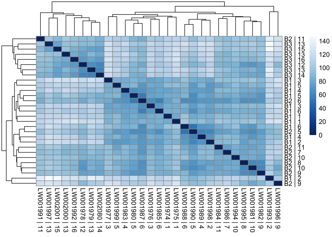
| Version | Author | Date |
|---|---|---|
| 08f6320 | sdhutchins | 2023-06-28 |
Principal Components Analysis
pcaData = plotPCA(vsd, intgroup=c("Batch", "Family", "Affected"), returnData=TRUE)
percentVar = round(100 * attr(pcaData, "percentVar"))

p1 <- ggplot(pcaData, aes(PC1, PC2, shape=factor(Batch), fill=factor(Affected),  color=factor(Family))) + geom_point(size=5) + xlab(paste0("PC1: ",percentVar[1],"% variance")) + ylab(paste0("PC2: ",percentVar[2],"% variance")) + coord_fixed()
p1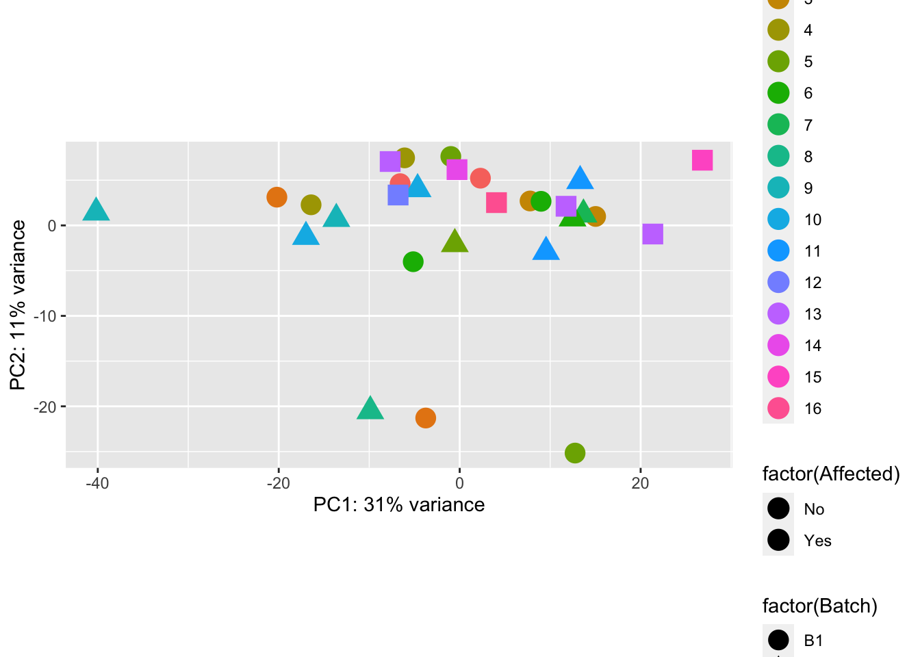
| Version | Author | Date |
|---|---|---|
| 08f6320 | sdhutchins | 2023-06-28 |
ggplot(pcaData, aes(PC1, PC2, shape=factor(Batch), color=factor(Affected)))  +
  geom_point(size=5) + xlab(paste0("PC1: ",percentVar[1],"% variance")) + ylab(paste0("PC2: ",percentVar[2],"% variance")) + coord_fixed()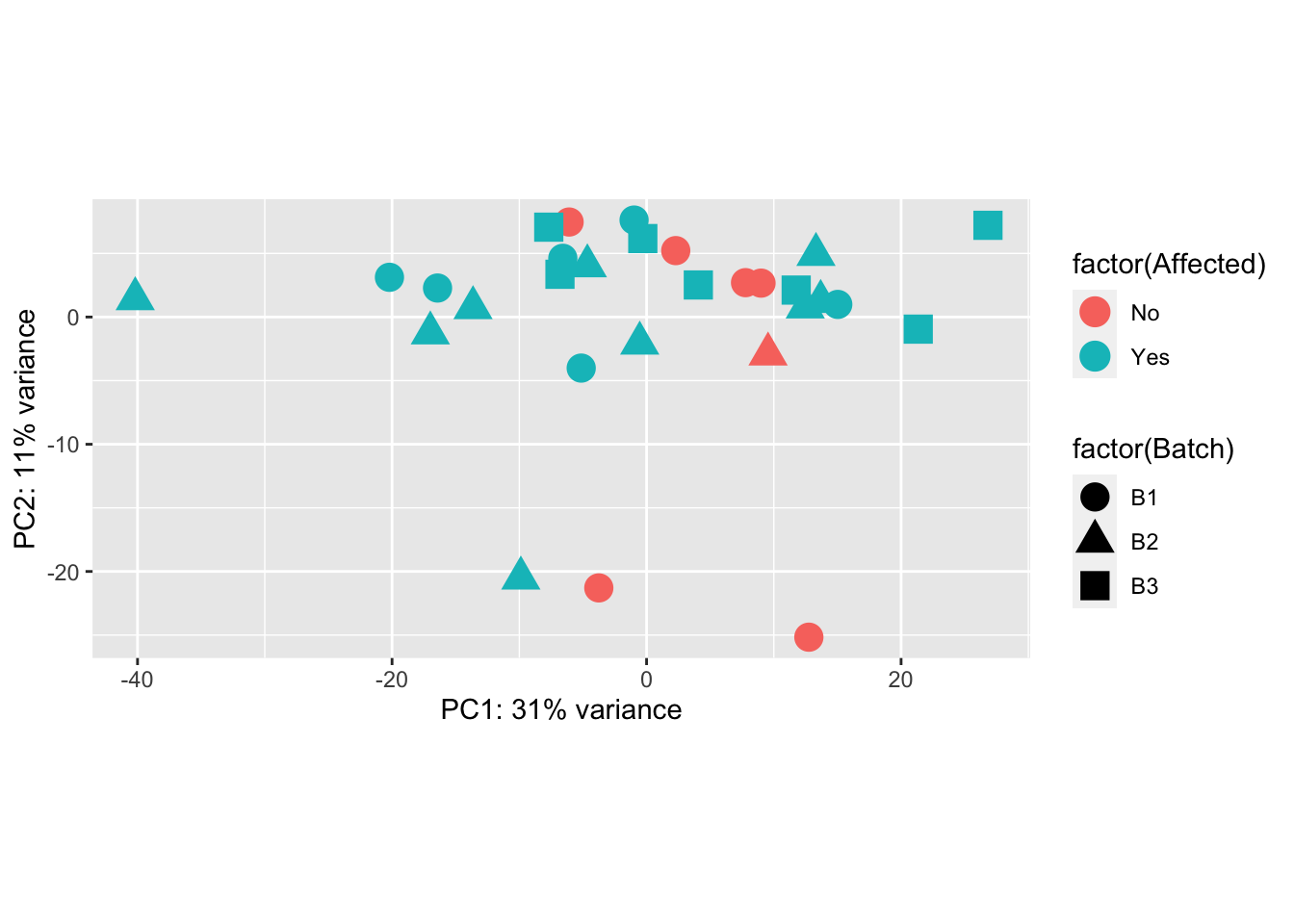
| Version | Author | Date |
|---|---|---|
| 08f6320 | sdhutchins | 2023-06-28 |
Heatmap of top 50 & top 100 genes
This is a heatmap for 50 genes with the highest variance across samples.
topVarGenes = head(order(-rowVars(assay(vsd))),50)
mat = assay(vsd_limma)[ topVarGenes, ]
mat = mat - rowMeans(mat)
df = as.data.frame(colData(vsd)[,c("Batch", "Affected")])
pheatmap(mat, annotation_col=df, fontsize = 5)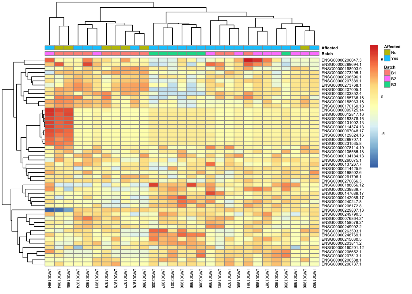
| Version | Author | Date |
|---|---|---|
| dbea49f | sdhutchins | 2023-06-27 |
This is a heatmap of the top 100 genes with the highest variance across samples.
topVarGenes = head(order(-rowVars(assay(vsd_limma))),100)
mat = assay(vsd_limma)[ topVarGenes, ]
mat = mat - rowMeans(mat)
df = as.data.frame(colData(vsd_limma)[,c("Batch", "Family", "Affected")])
pheatmap(mat, annotation_col=df, fontsize = 6)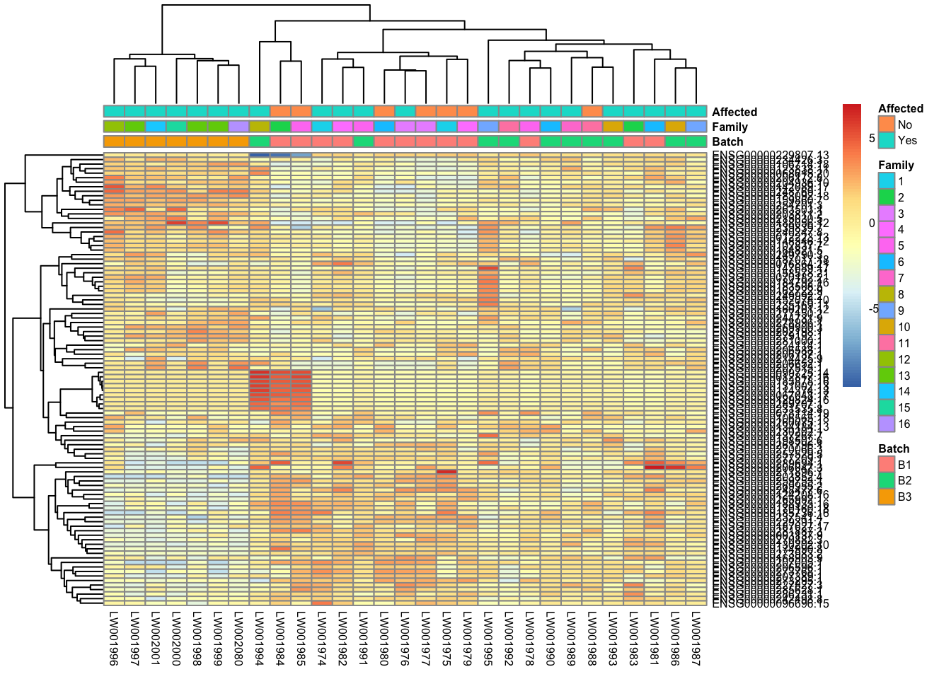
| Version | Author | Date |
|---|---|---|
| dbea49f | sdhutchins | 2023-06-27 |
Comparison/Contrast of Affected_Yes_vs_No
res_aff_vs_unaff = results(dds, contrast=c("Affected", "Yes", "No"))
res_aff_vs_unaff= res_aff_vs_unaff[order(res_aff_vs_unaff$padj),]
summary(res_aff_vs_unaff)
out of 29623 with nonzero total read count
adjusted p-value < 0.1
LFC > 0 (up)       : 20, 0.068%
LFC < 0 (down)     : 10, 0.034%
outliers [1]       : 134, 0.45%
low counts [2]     : 3997, 13%
(mean count < 1)
[1] see 'cooksCutoff' argument of ?results
[2] see 'independentFiltering' argument of ?resultswrite.csv(res_aff_vs_unaff, file="output/res_aff_vs_unaff.csv")
res_aff_vs_unaff_df = as.data.frame(res_aff_vs_unaff)
res_aff_vs_unaff_05 = subset(res_aff_vs_unaff_df, padj < 0.05) topgenes_byensemblid = head(rownames(res_aff_vs_unaff_05),50)
topgenes_aff_vs_unaff_05 = assay(vsd_limma)[topgenes_byensemblid,]
topgenes_aff_vs_unaff_05 = topgenes_aff_vs_unaff_05 - rowMeans(topgenes_aff_vs_unaff_05)
# Convert ensemblids
ensemblids <- topgenes_byensemblid
rownames(topgenes_aff_vs_unaff_05) <- gene_info$gene_name[match(ensemblids, gene_info$Ensembl_ID)]
topgenes_aff_vs_unaff_05 <- topgenes_aff_vs_unaff_05[order(row.names(topgenes_aff_vs_unaff_05)), ]
df = as.data.frame(colData(vsd_limma)[,c("Batch", "Family", "Affected")])
pheatmap(topgenes_aff_vs_unaff_05, annotation_col=df, fontsize = 5)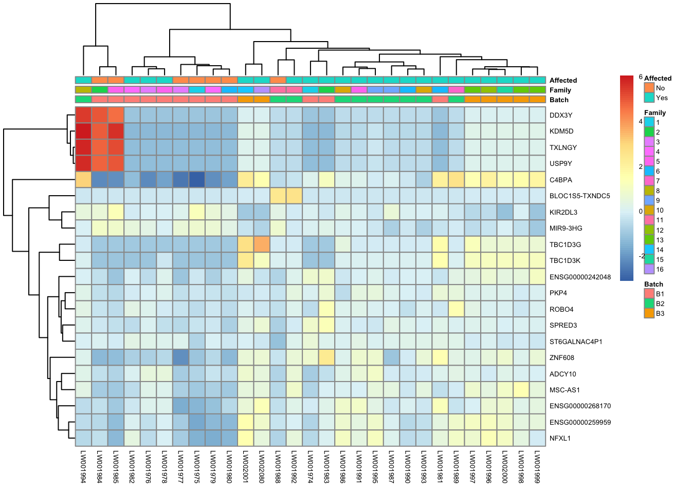
| Version | Author | Date |
|---|---|---|
| dbea49f | sdhutchins | 2023-06-27 |
res_aff_vs_unaff_df_genename = res_aff_vs_unaff_df
res_aff_vs_unaff_df_genename$Ensembl_ID = row.names(res_aff_vs_unaff_df)
res_aff_vs_unaff_df_genename = merge(x=res_aff_vs_unaff_df_genename, y=gene_info, by.x ="Ensembl_ID", by.y="Ensembl_ID", all.x=T)
res_aff_vs_unaff_df_genename = res_aff_vs_unaff_df_genename[,c(dim(res_aff_vs_unaff_df_genename)[2],1:dim(res_aff_vs_unaff_df_genename)[2]-1)]
res_aff_vs_unaff_df_genename = res_aff_vs_unaff_df_genename[order(res_aff_vs_unaff_df_genename[,"padj"]),]
write.csv(res_aff_vs_unaff_df_genename,file="output/res_aff_vs_unaff_genename.csv" )res_aff_vs_unaff_df_genename_05= subset(res_aff_vs_unaff_df_genename, padj < 0.05)
res_aff_vs_unaff_df_genename_05 = res_aff_vs_unaff_df_genename_05[order(res_aff_vs_unaff_df_genename_05$padj),]
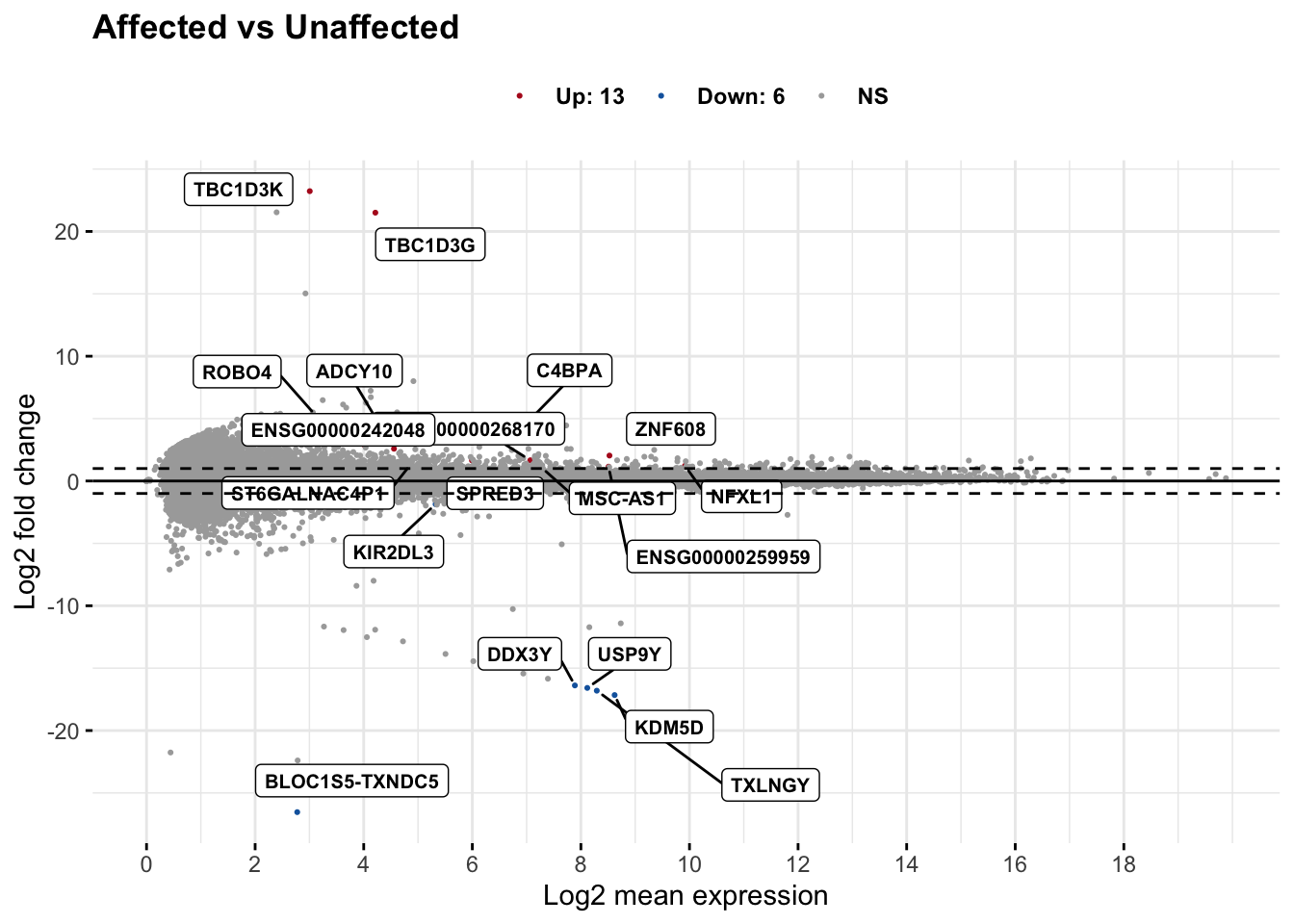
write.csv(res_aff_vs_unaff_df_genename_05, file="output/res_aff_vs_unaff_df_genename_05.csv")# Select specific genes to show
# set top = 0, then specify genes using label.select argument
ggmaplot(res_aff_vs_unaff_df_genename, main = "Affected vs Unaffected",
fdr = .05, fc = 2, size = 0.4,
genenames = as.vector(res_aff_vs_unaff_df_genename$gene_name),
ggtheme = ggplot2::theme_minimal(),
legend = "top", top = 19, font.label = c("bold", 8), label.rectangle = TRUE,
font.legend = "bold", font.main = "bold"
)
Enrichment analysis
Genes of Interest
genes_of_interest <- c("ACAD9/CFAP92", "ACADM", "ADORA2A", "ADRA1D", "ANKZF1", "AVPR1B", "CARMIL2", "CCDC178", "CENPF", "COQ2", "CR2", "DCTPP1", "DNASE1L3", "DPEP1", "EN03", "FCRL3", "FASTKD1", "GCKR", "GIMAP2", "HAGHL", "HSD11B1", "IRF2BP2", "KCNJ18", "LRCOL1", "LRBA, MAB21L2", "MFN1", "MRPS18B", "NLRP12", "P2RX7", "PGP", "PIEZO1", "PLCG2", "RERGL", "RPS6KC1", "SCN4A", "SIAE", "SLC11A2", "SLC12A3", "SLC4A1", "SLC6A12", "SLC9A9", "TDO2", "THEMIS", "TF", "TRAFD1", "UBASH3B", "WASHC5")

genes_interest_mart <- retrieve_gene_info(values = genes_of_interest, filters = "hgnc_symbol")

filtered_by_interest <- filter(res_aff_vs_unaff_df_genename, Ensembl_ID %in% genes_interest_mart$ensembl_gene_id_version)

filtered_by_interest
gene_name Ensembl_ID baseMean log2FoldChange lfcSE
1 SIAE ENSG00000110013.13 2.466639e+02 0.59408200 0.22599932
2 SLC9A9 ENSG00000181804.15 6.706541e+02 -0.55536081 0.24074420
3 MRPS18B ENSG00000204568.12 5.667532e+02 -0.31161333 0.14891684
4 SLC4A1 ENSG00000004939.16 5.296179e+04 0.90172281 0.56492353
5 DCTPP1 ENSG00000179958.10 2.499668e+02 -0.21356292 0.13908593
6 SCN4A ENSG00000007314.12 1.847233e+01 0.81871097 0.56661040
7 RPS6KC1 ENSG00000136643.12 8.229869e+02 -0.17255913 0.12415004
8 PIEZO1 ENSG00000103335.22 7.042958e+03 -0.18624466 0.13610317
9 TF ENSG00000091513.16 4.136235e+01 1.00864485 0.79068018
10 IRF2BP2 ENSG00000168264.11 5.613682e+03 -0.12180823 0.10830348
11 DNASE1L3 ENSG00000163687.14 2.668997e+01 0.63701556 0.60275359
12 COQ2 ENSG00000173085.15 3.108302e+02 0.16249033 0.15633871
13 HAGHL ENSG00000103253.19 1.498627e+02 -0.22565536 0.23901399
14 ADORA2A ENSG00000128271.22 1.283026e+03 -0.10698243 0.11661451
15 ANKZF1 ENSG00000163516.14 2.089193e+03 -0.09892576 0.10833298
16 GIMAP2 ENSG00000106560.11 1.683437e+03 -0.11941041 0.16565308
17 ACADM ENSG00000117054.15 1.035077e+03 0.09260737 0.14470412
18 HSD11B1 ENSG00000117594.10 4.069608e+00 0.56116575 0.98367616
19 PGP ENSG00000184207.9 6.671283e+02 -0.04890482 0.09161347
20 P2RX7 ENSG00000089041.17 1.019081e+03 0.09843146 0.19686960
21 SLC12A3 ENSG00000070915.10 3.199615e+01 -0.28589500 0.59193847
22 FASTKD1 ENSG00000138399.18 3.874435e+02 0.08135263 0.17507444
23 TRAFD1 ENSG00000135148.12 2.902964e+03 0.07679341 0.18963348
24 FCRL3 ENSG00000160856.21 1.711002e+03 0.13880061 0.35540614
25 THEMIS ENSG00000172673.12 1.674831e+03 -0.06364415 0.16796859
26 SLC11A2 ENSG00000110911.17 9.435833e+02 0.04955194 0.13329182
27 CARMIL2 ENSG00000159753.15 1.756139e+03 -0.05190117 0.19826345
28 SLC6A12 ENSG00000111181.13 1.512612e+02 -0.07875297 0.34108001
29 UBASH3B ENSG00000154127.10 1.728941e+03 -0.03073140 0.17865576
30 WASHC5 ENSG00000164961.16 1.394729e+03 -0.01778942 0.18565470
31 MFN1 ENSG00000171109.19 1.262655e+03 0.00887765 0.12420906
32 GCKR ENSG00000084734.9 4.139054e-01 0.83560399 2.78469874
stat pvalue padj
1 2.62868933 0.008571463 0.4327995
2 -2.30685020 0.021063172 0.5659292
3 -2.09253244 0.036390913 0.6195764
4 1.59618561 0.110447359 0.7261136
5 -1.53547470 0.124667268 0.7371881
6 1.44492753 0.148478244 0.7615943
7 -1.38992411 0.164551923 0.7714993
8 -1.36840799 0.171184403 0.7739906
9 1.27566730 0.202073154 0.7940612
10 -1.12469359 0.260718900 0.8269407
11 1.05684242 0.290583512 0.8382219
12 1.03934799 0.298642922 0.8427938
13 -0.94410945 0.345113720 0.8653454
14 -0.91740234 0.358931849 0.8706468
15 -0.91316382 0.361156387 0.8714518
16 -0.72084631 0.471004079 0.9046486
17 0.63997744 0.522187269 0.9169181
18 0.57047815 0.568353441 0.9280564
19 -0.53381695 0.593468184 0.9338074
20 0.49998305 0.617087012 0.9384532
21 -0.48298094 0.629109270 0.9413566
22 0.46467450 0.642164575 0.9427307
23 0.40495703 0.685509096 0.9527258
24 0.39054085 0.696136657 0.9552468
25 -0.37890509 0.704758348 0.9564953
26 0.37175526 0.710075075 0.9578674
27 -0.26177880 0.793491988 0.9716801
28 -0.23089294 0.817397976 0.9750350
29 -0.17201459 0.863426060 0.9809246
30 -0.09581991 0.923663606 0.9908813
31 0.07147345 0.943020953 0.9923648
32 0.30006980 0.764123917 NA
R version 4.1.1 (2021-08-10)
Platform: x86_64-apple-darwin17.0 (64-bit)
Running under: macOS Big Sur 10.16

Matrix products: default
BLAS:   /Library/Frameworks/R.framework/Versions/4.1/Resources/lib/libRblas.0.dylib
LAPACK: /Library/Frameworks/R.framework/Versions/4.1/Resources/lib/libRlapack.dylib

locale:
[1] en_US.UTF-8/en_US.UTF-8/en_US.UTF-8/C/en_US.UTF-8/en_US.UTF-8

attached base packages:
[1] stats4    stats     graphics  grDevices utils     datasets  methods
[8] base

other attached packages:
 [1] ggpubr_0.6.0                plotly_4.10.2
 [3] biomaRt_2.50.3              gprofiler2_0.2.2
 [5] limma_3.50.3                genefilter_1.76.0
 [7] pheatmap_1.0.12             RColorBrewer_1.1-3
 [9] DESeq2_1.34.0               SummarizedExperiment_1.24.0
[11] Biobase_2.54.0              MatrixGenerics_1.6.0
[13] matrixStats_1.0.0           GenomicRanges_1.46.1
[15] GenomeInfoDb_1.30.1         IRanges_2.28.0
[17] S4Vectors_0.32.4            BiocGenerics_0.40.0
[19] lubridate_1.9.2             forcats_1.0.0
[21] stringr_1.5.0               dplyr_1.1.2
[23] purrr_1.0.1                 readr_2.1.4
[25] tidyr_1.3.0                 tibble_3.2.1
[27] ggplot2_3.4.2.9000          tidyverse_2.0.0
[29] workflowr_1.7.0

loaded via a namespace (and not attached):
  [1] colorspace_2.1-0       ggsignif_0.6.4         ellipsis_0.3.2
  [4] rprojroot_2.0.3        XVector_0.34.0         fs_1.6.2
  [7] rstudioapi_0.14        farver_2.1.1           ggrepel_0.9.3
 [10] bit64_4.0.5            AnnotationDbi_1.56.2   fansi_1.0.4
 [13] xml2_1.3.4             splines_4.1.1          cachem_1.0.8
 [16] geneplotter_1.72.0     knitr_1.43             jsonlite_1.8.5
 [19] broom_1.0.5            annotate_1.72.0        dbplyr_2.3.2
 [22] png_0.1-8              shiny_1.7.4            compiler_4.1.1
 [25] httr_1.4.6             backports_1.4.1        Matrix_1.5-4.1
 [28] fastmap_1.1.1          lazyeval_0.2.2         cli_3.6.1
 [31] later_1.3.1            htmltools_0.5.5        prettyunits_1.1.1
 [34] tools_4.1.1            gtable_0.3.3           glue_1.6.2
 [37] GenomeInfoDbData_1.2.7 rappdirs_0.3.3         Rcpp_1.0.10
 [40] carData_3.0-5          jquerylib_0.1.4        vctrs_0.6.3
 [43] Biostrings_2.62.0      crosstalk_1.2.0        xfun_0.39
 [46] ps_1.7.5               mime_0.12              timechange_0.2.0
 [49] lifecycle_1.0.3        rstatix_0.7.2          XML_3.99-0.14
 [52] getPass_0.2-2          zlibbioc_1.40.0        scales_1.2.1
 [55] vroom_1.6.3            hms_1.1.3              promises_1.2.0.1
 [58] parallel_4.1.1         yaml_2.3.7             curl_5.0.1
 [61] memoise_2.0.1          sass_0.4.6             stringi_1.7.12
 [64] RSQLite_2.3.1          highr_0.10             filelock_1.0.2
 [67] BiocParallel_1.28.3    rlang_1.1.1            pkgconfig_2.0.3
 [70] bitops_1.0-7           evaluate_0.21          lattice_0.21-8
 [73] labeling_0.4.2         htmlwidgets_1.6.2      bit_4.0.5
 [76] processx_3.8.1         tidyselect_1.2.0       magrittr_2.0.3
 [79] R6_2.5.1               generics_0.1.3         DelayedArray_0.20.0
 [82] DBI_1.1.3              pillar_1.9.0           whisker_0.4.1
 [85] withr_2.5.0            abind_1.4-5            survival_3.5-5
 [88] KEGGREST_1.34.0        RCurl_1.98-1.12        car_3.1-2
 [91] crayon_1.5.2           utf8_1.2.3             BiocFileCache_2.2.1
 [94] tzdb_0.4.0             rmarkdown_2.22         progress_1.2.2
 [97] locfit_1.5-9.8         grid_4.1.1             data.table_1.14.8
[100] blob_1.2.4             callr_3.7.3            git2r_0.32.0
[103] digest_0.6.32          xtable_1.8-4           httpuv_1.6.11
[106] munsell_0.5.0          viridisLite_0.4.2      bslib_0.5.0