Last updated: 2020-11-19

Checks: 7 0

Knit directory: QuRIE-seq_manuscript/

This reproducible R Markdown analysis was created with workflowr (version 1.6.1). The Checks tab describes the reproducibility checks that were applied when the results were created. The Past versions tab lists the development history.


Great! Since the R Markdown file has been committed to the Git repository, you know the exact version of the code that produced these results.

Great job! The global environment was empty. Objects defined in the global environment can affect the analysis in your R Markdown file in unknown ways. For reproduciblity it’s best to always run the code in an empty environment.

The command set.seed(20201117) was run prior to running the code in the R Markdown file. Setting a seed ensures that any results that rely on randomness, e.g. subsampling or permutations, are reproducible.

Great job! Recording the operating system, R version, and package versions is critical for reproducibility.

Nice! There were no cached chunks for this analysis, so you can be confident that you successfully produced the results during this run.

Great job! Using relative paths to the files within your workflowr project makes it easier to run your code on other machines.

Great! You are using Git for version control. Tracking code development and connecting the code version to the results is critical for reproducibility.

The results in this page were generated with repository version 0cda3dc. See the Past versions tab to see a history of the changes made to the R Markdown and HTML files.

Note that you need to be careful to ensure that all relevant files for the analysis have been committed to Git prior to generating the results (you can use wflow_publish or wflow_git_commit). workflowr only checks the R Markdown file, but you know if there are other scripts or data files that it depends on. Below is the status of the Git repository when the results were generated:


Ignored files:
    Ignored:    .Rhistory
    Ignored:    .Rproj.user/

Untracked files:
    Untracked:  data/workflow_QuRIEseq.png.png
    Untracked:  output/MOFA_aIg.hdf5
    Untracked:  output/MOFA_aIg.rds
    Untracked:  output/data_weights_prot_fact1and3.csv
    Untracked:  output/metadata.csv
    Untracked:  output/paper_figures/
    Untracked:  output/seu_aIG_samples.rds
    Untracked:  output/seu_combined_filtered_allsamples.rds
    Untracked:  output/seu_combined_filtered_normalized.rds
    Untracked:  output/seu_combined_raw.rds
    Untracked:  output/seu_ibru_samples.rds

Unstaged changes:
    Modified:   analysis/MOFAibru.Rmd
    Modified:   code/load_packages.R

Note that any generated files, e.g. HTML, png, CSS, etc., are not included in this status report because it is ok for generated content to have uncommitted changes.


These are the previous versions of the repository in which changes were made to the R Markdown (analysis/MOFAaIg.Rmd) and HTML (docs/MOFAaIg.html) files. If you’ve configured a remote Git repository (see ?wflow_git_remote), click on the hyperlinks in the table below to view the files as they were in that past version.

File Version Author Date Message
Rmd 0cda3dc Jessie van Buggenum 2020-11-19 Figure 1 and 2 plus supplementary figures manuscript
html 2ffe38d Jessie van Buggenum 2020-11-17 Build site.
Rmd 4487750 Jessie van Buggenum 2020-11-17 basis set-up of page display
Rmd d9372d1 Jessie van Buggenum 2020-11-17 Publish the initial files for this website

source("code/load_packages.R")
seu_combined_selectsamples <- readRDS("output/seu_aIG_samples.rds")


panellabels <- c('a', 'b', 'c','d' , 'e', 'f', 'g', 'h', 'i', 'j', 'k')

add.textsize <- theme(axis.text.x = element_text(colour = 'black', size = 7),
          axis.text.y = element_text(colour = 'black',size=7),
          text = element_text(size=7),
          axis.text=element_text(size=7),
          plot.title = element_text(size=7)
          )


colorgradient6_manual <- c("#F7FBFF","#CFE1F2", "#93C4DE", "#4A97C9", "#1F5284", "#0C2236" )
colorgradient6_manual2 <- c("#d4d4d3","#CFE1F2", "#93C4DE", "#4A97C9", "#1F5284", "#0C2236" )
labels <- c("0", "2", "4", "6", "60", "180")

MOFA analysis time-series aIg

Variable features

Determine variable genes and proteins

seu_combined_selectsamples <- FindVariableFeatures(seu_combined_selectsamples, selection.method = "mvp", assay = "SCT.RNA", num.bin =20, mean.cutoff = c(0, 5), dispersion.cutoff = c(0.5,10), nfeatures =500)

genes.variable <- seu_combined_selectsamples@assays$SCT.RNA@var.features[-grep("^MT", seu_combined_selectsamples@assays$SCT.RNA@var.features)] # without the mitochondrial genes 

proteins.all <- row.names(seu_combined_selectsamples[["PROT"]])

meta.allcells <- seu_combined_selectsamples@meta.data %>%
  mutate(sample = rownames(seu_combined_selectsamples@meta.data))

MOFA model

## Note, if mofa object was generated before, it will read the generated rds file. (this will speed-up the process of generating this html document if edits are required)

myfiles <- list.files(path="output/", pattern = ".rds$")

if("MOFA_aIg.rds" %in%  myfiles){mofa <- readRDS("output/MOFA_aIg.rds")} else { #If so, read object, else do:
     
      mofa <- create_mofa(list(
        "RNA" = as.matrix( seu_combined_selectsamples@assays$SCT.RNA@scale.data[genes.variable,] ),
        "PROT" = as.matrix( seu_combined_selectsamples@assays$PROT@scale.data[proteins.all,] ))
        )

      # Default settings used (try 15 factors, excludes all non-informative factors)
      data_opts <- get_default_data_options(mofa)
      model_opts <- get_default_model_options(mofa)
      train_opts <- get_default_training_options(mofa)
      train_opts$seed <- 42 # use same seed for reproducibility
      mofa <- prepare_mofa(
        object = mofa,
        data_options = data_opts,
        model_options = model_opts,
        training_options = train_opts
        )

    mofa <- run_mofa(mofa, outfile = "output/MOFA_aIg.hdf5")
    mofa <- run_umap(mofa, factors = c(1:7))
    samples_metadata(mofa) <- meta.allcells
    saveRDS(mofa, file= "output/MOFA_aIg.rds")
  
}


mofa
Trained MOFA with the following characteristics: 
 Number of views: 2 
 Views names: RNA PROT 
 Number of features (per view): 2371 80 
 Number of groups: 1 
 Groups names: group1 
 Number of samples (per group): 4767 
 Number of factors: 9 
# Export Factor 1 and 3 weights for Cytoscape plot
data_weights_prot <- get_weights(object = mofa, views = "PROT", factors = c(1,3), as.data.frame = TRUE)

data_weights_prot <- as.data.frame(data_weights_prot)  %>%
  spread(factor, value) %>%
  mutate(Factor1_signflip = Factor1 *-1)

write.csv2(data_weights_prot, file = "output/data_weights_prot_fact1and3.csv")

Figure 1

UMAP on 7 MOFA factors

## UMAP
plot.umap.data <-  plot_dimred(mofa, method="UMAP", color_by = "condition",stroke = 0.001, dot_size =1, alpha = 0.2, return_data = T)

plot.umap.all <- ggplot(plot.umap.data, aes(x=x, y = y, fill = color_by))+
  geom_point(size = 0.8, alpha = 0.6, shape = 21, stroke = 0) +
  theme_half_open() +
  scale_fill_manual(values = colorgradient6_manual, labels = c(labels), name = "Time aIg",)+
   theme(legend.position="none")+
  add.textsize +
  labs(title = "UMAP on MOFA+ factors shows minute and \nhour time-scale cell-state transitions", x = "UMAP 1", y = "UMAP 2")

## UMAP legend
legend.umap <- get_legend( ggplot(plot.umap.data, aes(x=x, y = y, fill = color_by))+
  geom_point(size = 2, alpha = 1, shape = 21, stroke = 0) +
  theme_half_open() +
  scale_fill_manual(values = colorgradient6_manual, labels = c(labels), name = "Time aIg \n(minutes)",)+
  add.textsize +
  labs(title = "UMAP on MOFA+ factors shows minute and \nhour time-scale cell-state transitions", x = "UMAP 1", "y = UMAP 2"))
legend.umap <- as_ggplot(legend.umap)
plot_fig1_umap <- plot_grid(plot.umap.all,legend.umap, labels = c(""), label_size = 10, ncol = 2, rel_widths = c(1, 0.2))

ggsave(plot_fig1_umap, filename = "output/paper_figures/Fig1_UMAP.pdf", width = 68, height = 62, units = "mm",  dpi = 300, useDingbats = FALSE)
ggsave(plot_fig1_umap, filename = "output/paper_figures/Fig1_UMAP.png", width = 68, height = 62, units = "mm",  dpi = 300)

plot_fig1_umap

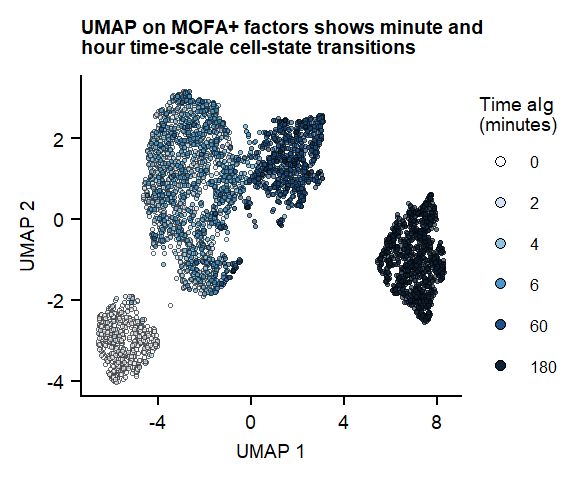
Figure 1. UMAP of 7 MOFA factors, integrating phospho-protein and RNA measurements

Suppl PCA

seu_combined_selectsamples <- RunPCA(seu_combined_selectsamples,assay = "SCT.RNA", features = genes.variable, verbose = FALSE, ndims.print = 0, reduction.name = "pca.RNA")
seu_combined_selectsamples <- RunPCA(seu_combined_selectsamples, assay = "PROT", features = proteins.all, verbose = FALSE, ndims.print = 0,reduction.name = "pca.PROT")
## PCA analysis

plot.PCA.RNA <- DimPlot(seu_combined_selectsamples, reduction = "pca.RNA", group.by = "condition", pt.size =0.2) +
  scale_color_manual(values = colorgradient6_manual2, labels = c(labels), name = "Time aIg",)+
  labs(title = "RNA PCA separates cells \nat hour time-scale", x= "RNA PC 1", y = " RNA PC 2") +
  add.textsize +
  theme(legend.position = "none")


plot.PCA.PROT <- DimPlot(seu_combined_selectsamples, reduction = "pca.PROT", group.by = "condition", pt.size = 0.2) +
  scale_color_manual(values = colorgradient6_manual2, labels = c(labels), name = "Time aIg",)+
  labs(title = "(phospho-)protein PCA separates cells\nat minutes time-scale", x= "Protein PC 1", y = "Protein PC 2") +
  add.textsize +
  #  scale_x_reverse()+
  theme(legend.position = "none")

legend <- get_legend(DimPlot(seu_combined_selectsamples, reduction = "pca.RNA", group.by = "condition", pt.size =0.1) +
  scale_color_manual(values = colorgradient6_manual2, labels = c(labels), name = "Time aIg",)+
  add.textsize)
legend <- as_ggplot(legend)


PCA.PROTPC1.data <- data.frame(rank = 1:80, 
                               protein = names(sort(seu_combined_selectsamples@reductions$pca.PROT@feature.loadings[,1])),
                               weight.PC1 = sort(seu_combined_selectsamples@reductions$pca.PROT@feature.loadings[,1]),
                               highlights = c(names(sort(seu_combined_selectsamples@reductions$pca.PROT@feature.loadings[,1]))[1:4],rep("",76))
                               ) 

plot.PCA.PROTweightsPC1 <- ggplot(PCA.PROTPC1.data, aes(x=weight.PC1, y = rank, label = highlights)) +
  geom_point(size=0.1) +
  labs(title = "Top 4 protein loadings \n", x= "Weight Protein PC1") +
  geom_point(color = ifelse(PCA.PROTPC1.data$highlights == "", "grey50", "red")) +
  geom_text_repel(size = 2, segment.size = 0.25)+
  theme_half_open()+
  add.textsize +
  theme(axis.title.y=element_blank(),
        axis.text.y=element_blank(),
        axis.ticks.y=element_blank()
        ) +
  scale_x_reverse()+
  scale_y_reverse()


PCA.RNAPC1.data <- data.frame(rank = 1:2371, 
                               RNA = names(sort(seu_combined_selectsamples@reductions$pca.RNA@feature.loadings[,1])),
                               weight.PC1 = sort(seu_combined_selectsamples@reductions$pca.RNA@feature.loadings[,1]),
                               highlights = c(rep("",2366),names(sort(seu_combined_selectsamples@reductions$pca.RNA@feature.loadings[,1]))[2367:2371])
                               ) 
## Loadings RNA
plot.PCA.RNAweightsPC1 <- ggplot(PCA.RNAPC1.data, aes(x=weight.PC1, y = rank, label = highlights)) +
  geom_point(size=0.1) +
  labs(title = "Top 4 RNA loadings \n", x= "Weight RNA PC1") +
  geom_point(color = ifelse(PCA.RNAPC1.data$highlights == "", "grey50", "red")) +
  geom_text_repel(size = 2, segment.size = 0.25)+
  theme_half_open()+
  add.textsize +
  theme(axis.title.y=element_blank(),
        axis.text.y=element_blank(),
        axis.ticks.y=element_blank()
        ) 

## ridgeplots
PC1.data <- data.frame(sample = rownames(seu_combined_selectsamples@reductions$pca.PROT@cell.embeddings),
                       PC1_PROT = seu_combined_selectsamples@reductions$pca.PROT@cell.embeddings[,1],
                       PC1_RNA = seu_combined_selectsamples@reductions$pca.RNA@cell.embeddings[,1]) %>%
  left_join(meta.allcells)

plot_ridge_PC1Prot <- ggplot(PC1.data, aes(x = PC1_PROT, y = condition, fill = condition)) + 
  scale_fill_manual(values = colorgradient6_manual, labels = c(labels), name = "Time aIg \n(minutes)")+
  geom_density_ridges2() +
  scale_y_discrete(labels = labels,  name = "Time aIg (minutes)")+
  scale_x_continuous(name = "PC1 Proteins") +
  theme_half_open() +
  add.textsize+
  theme(legend.position = "none")

plot_ridge_PC1RNA <- ggplot(PC1.data, aes(x = PC1_RNA, y = condition, fill = condition)) + 
  scale_fill_manual(values = colorgradient6_manual, labels = c(labels), name = "Time aIg \n(minutes)")+
  geom_density_ridges2() +
  scale_y_discrete(labels = labels,  name = "Time aIg (minutes)")+
  scale_x_continuous(name = "PC1 RNA") +
  theme_half_open() +
  add.textsize+
  theme(legend.position = "none")
Fig1.pca <- plot_grid(plot.PCA.PROT,plot.PCA.RNA,legend, plot_ridge_PC1Prot, plot_ridge_PC1RNA,NULL,  plot.PCA.PROTweightsPC1, plot.PCA.RNAweightsPC1, labels = c(panellabels[1:2], "","","","",panellabels[3:4]), label_size = 10, ncol = 3, rel_widths = c(0.9,0.9,0.2,0.9,0.9), rel_heights = c(1,0.8,1.3))
Picking joint bandwidth of 0.37
Picking joint bandwidth of 0.368
ggsave(filename = "output/paper_figures/Suppl_PCA_aIg.pdf", width = 143, height = 170, units = "mm",  dpi = 300, useDingbats = FALSE)
ggsave(filename = "output/paper_figures/Suppl_PCA_aIg.png", width = 143, height = 170, units = "mm",  dpi = 300)

Fig1.pca

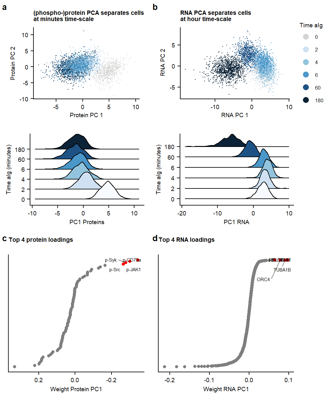
Supplemental Figure. PCA analysis on RNA ór Protein dataset

Suppl MOFA model properties

Fig.1.suppl.mofa.row1 <- plot_grid(plot.variance.perfactor.all, plot.variance.total,NULL, plot.heatmap.pval.covariates, labels = c(panellabels[1:3]), label_size = 10, ncol = 4, rel_widths = c(1.35, 0.27,0.2,0.38))

Fig.1.suppl.mofa.row2 <- plot_grid(plot.violin.factorall,legend.umap, labels = panellabels[4], label_size = 10, ncol = 2, rel_widths = c(1,0.1))

Suppl_mofa <- plot_grid(Fig.1.suppl.mofa.row1, Fig.1.suppl.mofa.row2, plot.rank.PROT.2.4to7, plot.rank.RNA.2.4to7, labels = c("","", panellabels[5:6]),label_size = 10, ncol = 1, rel_heights = c(1.45,1,1.1,1.1))


ggsave(Suppl_mofa, filename = "output/paper_figures/Suppl_MOFAaIg.pdf", width = 183, height = 220, units = "mm",  dpi = 300, useDingbats = FALSE)
ggsave(Suppl_mofa, filename = "output/paper_figures/Suppl_MOFAaIg.png", width = 183, height = 220, units = "mm",  dpi = 300)

Suppl_mofa

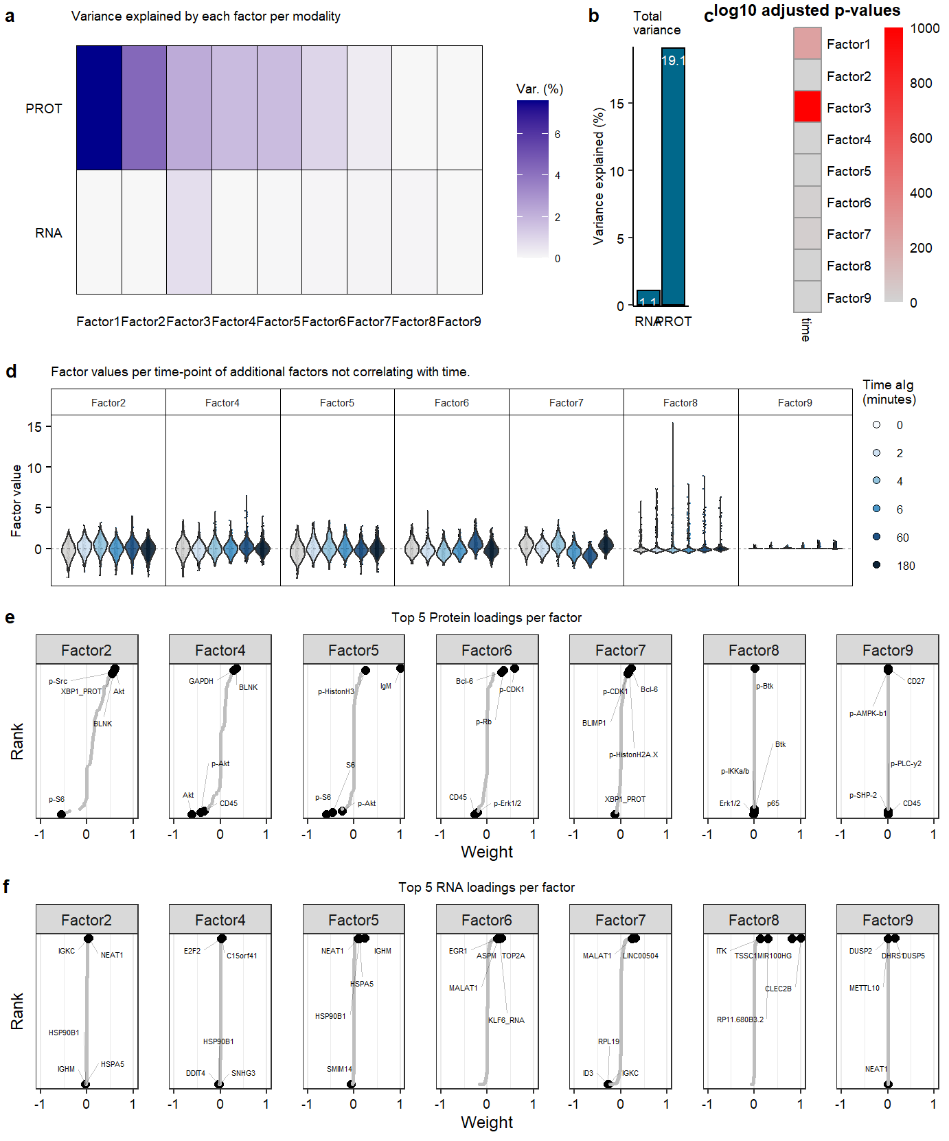
Supplemental Figure. MOFA model additional information

Figure 2

Prepare main panels

Enrichment analysis of Factor 3 positive loadings

topposrna.factor3 <- weights.RNA %>%
  filter(factor == "Factor3" & value >= 0) %>%
  arrange(-value)
rownames(topposrna.factor3) <- topposrna.factor3$feature

### Convert Gene-names to gene IDs (using 'org.Hs.eg.db' library)

topposrna.factor3 <- topposrna.factor3 %>%
  mutate(ENTREZID = mapIds(org.Hs.eg.db, as.character(topposrna.factor3$feature), 'ENTREZID', 'SYMBOL'))
'select()' returned 1:1 mapping between keys and columns
listgenes.factor3 <- topposrna.factor3$value

names(listgenes.factor3) <- topposrna.factor3$ENTREZID


go.pb.fct3.pos <- enrichGO(gene         = topposrna.factor3$feature,
                OrgDb         = org.Hs.eg.db,
                keyType       = 'SYMBOL',
                ont           = "BP",
                pAdjustMethod = "BH")

go.pb.fct3.pos <- simplify(go.pb.fct3.pos, cutoff=0.6, by="p.adjust", select_fun=min)


go.pb.fct3.pos.dplyr <- mutate(go.pb.fct3.pos, richFactor = Count / as.numeric(sub("/\\d+", "", BgRatio))) 

## plot main panel
plot.enriched.go.bp.factor3 <- ggplot(go.pb.fct3.pos.dplyr, showCategory = 10, 
  aes(-log10(p.adjust), fct_reorder(Description,  -log10(p.adjust)))) +   geom_segment(aes(xend=0, yend = Description)) +
  geom_point(aes(size = Count)) +
  scale_color_viridis_c(guide=guide_colorbar(reverse=TRUE)) +
  scale_size_continuous(range=c(0.5, 3)) +
  theme_minimal() + 
  add.textsize +
  xlab("-log adj pval") +
  ylab(NULL) + 
  ggtitle("Enriched Biological Processes") +
  theme(legend.position="none")

legend.plot.enriched.go.bp.factor3 <- as.ggplot(get_legend(ggplot(go.pb.fct3.pos.dplyr, showCategory = 10, 
  aes(-log10(p.adjust), fct_reorder(Description,  -log10(p.adjust)))) +   geom_segment(aes(xend=0, yend = Description)) +
  geom_point(aes(size = Count)) +
  scale_color_viridis_c(guide=guide_colorbar(reverse=TRUE)) +
  scale_size_continuous(range=c(0.5, 3)) +
  theme_minimal() + 
  add.textsize +
  xlab("-log adj pval") +
  ylab(NULL) + 
  ggtitle("Enriched Biological Processes") +
     theme(legend.position="right")))

## Plot supplementary
plot.enriched.go.bp.factor3_50 <- ggplot(go.pb.fct3.pos.dplyr, showCategory = 50, 
  aes(-log10(p.adjust), fct_reorder(Description,  -log10(p.adjust)))) +   geom_segment(aes(xend=0, yend = Description)) +
  geom_point(aes(size = Count)) +
  scale_color_viridis_c(guide=guide_colorbar(reverse=TRUE)) +
  scale_size_continuous(range=c(0.5, 3)) +
  theme_minimal() + 
  add.textsize +
  xlab("-log adj pval") +
  ylab(NULL) + 
  ggtitle("Enriched Biological Processes") 
message(c("Significance protein folding GO term: \n",go.pb.fct3.pos.dplyr@result[which(go.pb.fct3.pos.dplyr@result$Description == "protein folding"),"p.adjust"]))
Significance protein folding GO term: 
0.0210693865776273

Main figure 2

Fig2.row1.violinsprot <- plot_grid(`plot.violin.p-CD79a`, `plot.violin.p-Syk`, `plot.violin.p-JAK1`,labels = c(panellabels[3]), label_size = 10, ncol = 1, rel_heights = c(1.2,0.95,1.2))
Fig2.row1 <- plot_grid(plot.violin.factor1,plot.rank.PROT.1, plot.rank.RNA.1, Fig2.row1.violinsprot, labels = c(panellabels[1:2], ""),  label_size = 10, ncol =4, rel_widths = c(0.8,0.55,0.5,0.8))

Fig2.row2.violinsrna <- plot_grid(plot.violin.rna.NEAT1,plot.violin.rna.NPM1, plot.violin.rna.BTF3,labels = "", label_size = 10, ncol = 1, rel_heights = c(1.2,0.95,1.2))

Fig2.row2 <- plot_grid(plot.violin.factor3,plot.rank.PROT.3,plot.rank.RNA.3,Fig2.row2.violinsrna, labels = c(panellabels[4:5], "", panellabels[7]), label_size = 10, ncol =4, rel_widths = c(0.8,0.55,0.5,0.8))

Fig2.row3 <- plot_grid(plot.enriched.go.bp.factor3,legend.plot.enriched.go.bp.factor3,NULL, labels = panellabels[6], label_size = 10, ncol =3, rel_widths = c(1.8,0.2,0.6))

plot_fig2 <- plot_grid(Fig2.row1, Fig2.row2,Fig2.row3, labels = c("", "", ""), label_size = 10, ncol = 1, rel_heights = c(1,1,0.55))

ggsave(plot_fig2, filename = "output/paper_figures/Fig2.pdf", width = 183, height = 183, units = "mm",  dpi = 300, useDingbats = FALSE)
ggsave(plot_fig2, filename = "output/paper_figures/Fig2.png", width = 183, height = 183, units = "mm",  dpi = 300)

plot_fig2

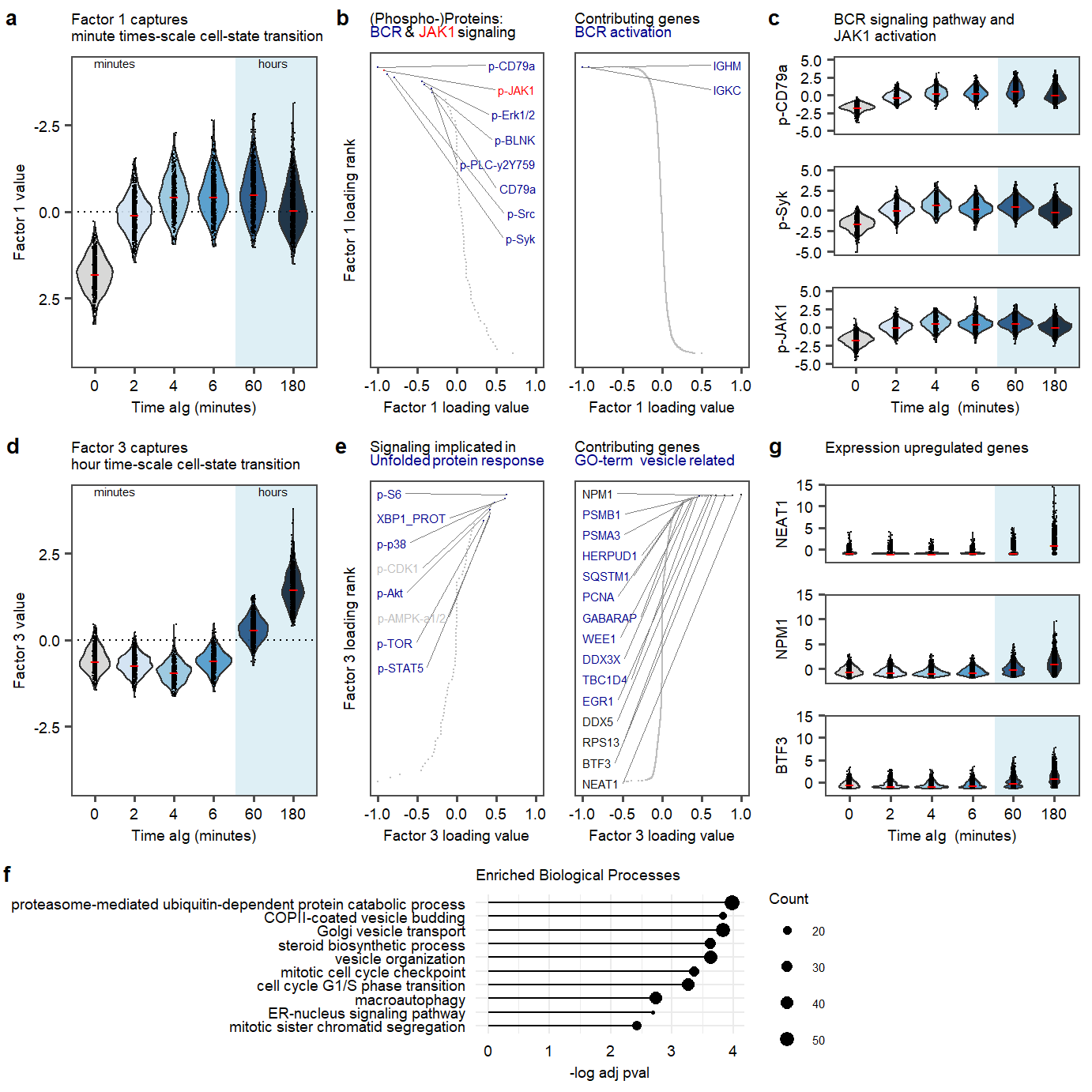
Figure 2. Factor 1 and 3 exploration.

Suppl Enriched Fact 3

ggsave(plot.enriched.go.bp.factor3_50, filename = "output/paper_figures/Suppl_Enrichm_Fct3.pdf", width = 183, height = 183, units = "mm",  dpi = 300, useDingbats = FALSE)
ggsave(plot.enriched.go.bp.factor3_50, filename = "output/paper_figures/Suppl_Enrichm_Fct3.png", width = 183, height = 183, units = "mm",  dpi = 300)
plot.enriched.go.bp.factor3_50

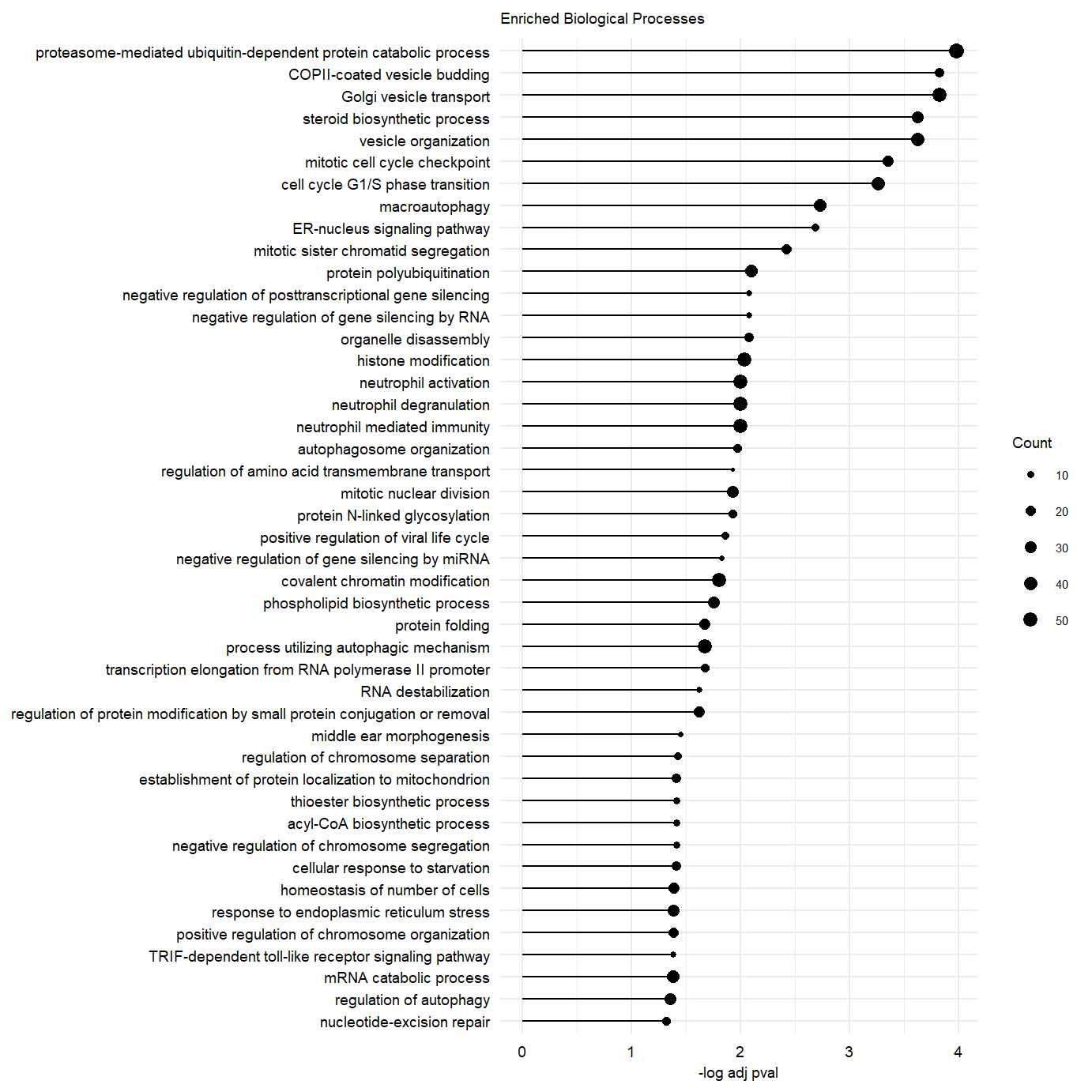
Supplemental Figure. Top 50 enriched gene-sets in postive loadings factor 3.


sessionInfo()
R version 3.6.3 (2020-02-29)
Platform: x86_64-w64-mingw32/x64 (64-bit)
Running under: Windows 10 x64 (build 17763)

Matrix products: default

locale:
[1] LC_COLLATE=English_Netherlands.1252  LC_CTYPE=English_Netherlands.1252   
[3] LC_MONETARY=English_Netherlands.1252 LC_NUMERIC=C                        
[5] LC_TIME=English_Netherlands.1252    

attached base packages:
 [1] parallel  stats4    grid      stats     graphics  grDevices utils    
 [8] datasets  methods   base     

other attached packages:
 [1] png_0.1-7                   forcats_0.5.0              
 [3] clusterProfiler_3.14.3      clusterProfiler.dplyr_0.0.2
 [5] enrichplot_1.6.1            org.Hs.eg.db_3.10.0        
 [7] AnnotationDbi_1.48.0        IRanges_2.20.2             
 [9] S4Vectors_0.24.4            Biobase_2.46.0             
[11] BiocGenerics_0.32.0         ggridges_0.5.2             
[13] cowplot_1.1.0               ggtext_0.1.0               
[15] ggplotify_0.0.5             ggcorrplot_0.1.3           
[17] ggrepel_0.8.2               ggpubr_0.4.0               
[19] scico_1.2.0                 MOFA2_1.1                  
[21] extrafont_0.17              patchwork_1.0.1            
[23] RColorBrewer_1.1-2          viridis_0.5.1              
[25] viridisLite_0.3.0           ggsci_2.9                  
[27] sctransform_0.3.1           ggthemes_4.2.0             
[29] matrixStats_0.57.0          kableExtra_1.2.1           
[31] gridExtra_2.3               Seurat_3.2.2               
[33] ggplot2_3.3.2               scales_1.1.1               
[35] tidyr_1.1.2                 dplyr_1.0.2                
[37] stringr_1.4.0               workflowr_1.6.1            

loaded via a namespace (and not attached):
  [1] reticulate_1.16       tidyselect_1.1.0      RSQLite_2.2.1        
  [4] htmlwidgets_1.5.2     BiocParallel_1.20.1   Rtsne_0.15           
  [7] munsell_0.5.0         codetools_0.2-16      ica_1.0-2            
 [10] future_1.19.1         miniUI_0.1.1.1        withr_2.3.0          
 [13] GOSemSim_2.12.1       colorspace_1.4-1      knitr_1.30           
 [16] rstudioapi_0.11       ROCR_1.0-11           ggsignif_0.6.0       
 [19] tensor_1.5            DOSE_3.12.0           Rttf2pt1_1.3.8       
 [22] listenv_0.8.0         labeling_0.4.2        git2r_0.27.1         
 [25] urltools_1.7.3        mnormt_2.0.2          polyclip_1.10-0      
 [28] farver_2.0.3          bit64_4.0.5           pheatmap_1.0.12      
 [31] rhdf5_2.30.1          rprojroot_1.3-2       vctrs_0.3.4          
 [34] generics_0.0.2        xfun_0.18             markdown_1.1         
 [37] R6_2.4.1              graphlayouts_0.7.0    rsvd_1.0.3           
 [40] fgsea_1.12.0          spatstat.utils_1.17-0 gridGraphics_0.5-0   
 [43] DelayedArray_0.12.3   promises_1.1.0        ggraph_2.0.3         
 [46] gtable_0.3.0          globals_0.13.1        goftest_1.2-2        
 [49] tidygraph_1.2.0       rlang_0.4.8           splines_3.6.3        
 [52] rstatix_0.6.0         extrafontdb_1.0       lazyeval_0.2.2       
 [55] europepmc_0.4         broom_0.7.1           BiocManager_1.30.10  
 [58] yaml_2.2.1            reshape2_1.4.4        abind_1.4-5          
 [61] backports_1.1.10      httpuv_1.5.2          qvalue_2.18.0        
 [64] gridtext_0.1.1        tools_3.6.3           psych_2.0.9          
 [67] ellipsis_0.3.1        Rcpp_1.0.4.6          plyr_1.8.6           
 [70] progress_1.2.2        purrr_0.3.4           prettyunits_1.1.1    
 [73] rpart_4.1-15          deldir_0.1-29         pbapply_1.4-3        
 [76] zoo_1.8-8             haven_2.3.1           cluster_2.1.0        
 [79] fs_1.4.1              magrittr_1.5          data.table_1.13.0    
 [82] DO.db_2.9             openxlsx_4.2.2        triebeard_0.3.0      
 [85] lmtest_0.9-38         RANN_2.6.1            tmvnsim_1.0-2        
 [88] whisker_0.4           fitdistrplus_1.1-1    hms_0.5.3            
 [91] mime_0.9              evaluate_0.14         xtable_1.8-4         
 [94] rio_0.5.16            readxl_1.3.1          compiler_3.6.3       
 [97] tibble_3.0.4          KernSmooth_2.23-16    crayon_1.3.4         
[100] htmltools_0.5.0       mgcv_1.8-31           later_1.0.0          
[103] DBI_1.1.0             tweenr_1.0.1          corrplot_0.84        
[106] MASS_7.3-53           rappdirs_0.3.1        Matrix_1.2-18        
[109] car_3.0-10            igraph_1.2.6          pkgconfig_2.0.3      
[112] rvcheck_0.1.8         foreign_0.8-75        plotly_4.9.2.1       
[115] xml2_1.3.2            webshot_0.5.2         rvest_0.3.6          
[118] digest_0.6.26         RcppAnnoy_0.0.16      spatstat.data_1.4-3  
[121] fastmatch_1.1-0       rmarkdown_2.4         cellranger_1.1.0     
[124] leiden_0.3.3          uwot_0.1.8            curl_4.3             
[127] shiny_1.5.0           lifecycle_0.2.0       nlme_3.1-144         
[130] jsonlite_1.7.1        Rhdf5lib_1.8.0        carData_3.0-4        
[133] pillar_1.4.6          lattice_0.20-38       GO.db_3.10.0         
[136] fastmap_1.0.1         httr_1.4.2            survival_3.1-8       
[139] glue_1.4.2            zip_2.1.1             spatstat_1.64-1      
[142] bit_4.0.4             ggforce_0.3.2         stringi_1.4.6        
[145] HDF5Array_1.14.4      blob_1.2.1            memoise_1.1.0        
[148] irlba_2.3.3           future.apply_1.6.0