Last updated: 2021-06-14

Checks: 7 0

Knit directory: QuRIE-seq_manuscript/

This reproducible R Markdown analysis was created with workflowr (version 1.6.2). The Checks tab describes the reproducibility checks that were applied when the results were created. The Past versions tab lists the development history.


Great! Since the R Markdown file has been committed to the Git repository, you know the exact version of the code that produced these results.

Great job! The global environment was empty. Objects defined in the global environment can affect the analysis in your R Markdown file in unknown ways. For reproduciblity it’s best to always run the code in an empty environment.

The command set.seed(20201117) was run prior to running the code in the R Markdown file. Setting a seed ensures that any results that rely on randomness, e.g. subsampling or permutations, are reproducible.

Great job! Recording the operating system, R version, and package versions is critical for reproducibility.

Nice! There were no cached chunks for this analysis, so you can be confident that you successfully produced the results during this run.

Great job! Using relative paths to the files within your workflowr project makes it easier to run your code on other machines.

Great! You are using Git for version control. Tracking code development and connecting the code version to the results is critical for reproducibility.

The results in this page were generated with repository version 35e992e. See the Past versions tab to see a history of the changes made to the R Markdown and HTML files.

Note that you need to be careful to ensure that all relevant files for the analysis have been committed to Git prior to generating the results (you can use wflow_publish or wflow_git_commit). workflowr only checks the R Markdown file, but you know if there are other scripts or data files that it depends on. Below is the status of the Git repository when the results were generated:


Ignored files:
    Ignored:    .Rhistory
    Ignored:    .Rproj.user/
    Ignored:    data/raw/
    Ignored:    output/MOFA_aIg.hdf5
    Ignored:    output/MOFA_aIg.rds
    Ignored:    output/MOFA_ibru.hdf5
    Ignored:    output/MOFA_ibru.rds
    Ignored:    output/data_weights_prot_fact1and3.csv
    Ignored:    output/metadata.csv
    Ignored:    output/metadata_Ricard.csv
    Ignored:    output/paper_figures/
    Ignored:    output/seu_aIG_samples.rds
    Ignored:    output/seu_combined_filtered_normalized.rds
    Ignored:    output/seu_combined_raw.rds
    Ignored:    output/seu_ibru_samples.rds

Unstaged changes:
    Modified:   analysis/revisions.rmd

Note that any generated files, e.g. HTML, png, CSS, etc., are not included in this status report because it is ok for generated content to have uncommitted changes.


These are the previous versions of the repository in which changes were made to the R Markdown (analysis/MOFAibru.Rmd) and HTML (docs/MOFAibru.html) files. If you’ve configured a remote Git repository (see ?wflow_git_remote), click on the hyperlinks in the table below to view the files as they were in that past version.

File Version Author Date Message
html 346674a Jessie van Buggenum 2020-12-01 Build site.
Rmd b7053b8 Jessie van Buggenum 2020-12-01 small typo edits panel titles
html 73a9ca0 Jessie van Buggenum 2020-12-01 Build site.
Rmd 5ba7d07 Jessie van Buggenum 2020-12-01 small edits panel titles
html 84d2210 Jessie van Buggenum 2020-11-26 Build site.
Rmd ca0d35d Jessie van Buggenum 2020-11-26 update ibru to Ibru
html b822e81 Jessie van Buggenum 2020-11-26 Build site.
Rmd cdfdb86 Jessie van Buggenum 2020-11-26 update ibru to Ibru
html d8ba888 Jessie van Buggenum 2020-11-26 Build site.
Rmd 1d2b544 Jessie van Buggenum 2020-11-26 minor change to capitalization of protein names
html bbd8940 Jessie van Buggenum 2020-11-26 Build site.
Rmd be4b610 Jessie van Buggenum 2020-11-26 Capitalize several proteins in all plots (hardcoded)
html 61cb954 Jessie van Buggenum 2020-11-25 Build site.
Rmd cf646e0 Jessie van Buggenum 2020-11-25 typo Syk to SYK
html 416c6ae Jessie van Buggenum 2020-11-24 Build site.
Rmd 2290baf Jessie van Buggenum 2020-11-24 hide figure panels in html
html 8e6f68c Jessie van Buggenum 2020-11-24 Build site.
Rmd 4b4ea4c Jessie van Buggenum 2020-11-24 update minor changes to documentation and suppl fig
html 2412f7d Jessie van Buggenum 2020-11-24 Build site.
Rmd 8d11c04 Jessie van Buggenum 2020-11-24 Documentation Figure 3: ibrutinib data
html 2ffe38d Jessie van Buggenum 2020-11-17 Build site.
Rmd 4487750 Jessie van Buggenum 2020-11-17 basis set-up of page display
Rmd d9372d1 Jessie van Buggenum 2020-11-17 Publish the initial files for this website

source("code/load_packages.R")

panellabels <- c('a', 'b', 'c','d' , 'e', 'f', 'g', 'h', 'i', 'j', 'k')

add.textsize <- theme(axis.text.x = element_text(colour = 'black', size = 7),
          axis.text.y = element_text(colour = 'black',size=7),
          text = element_text(size=7),
          axis.text=element_text(size=7),
          plot.title = element_text(size=7)
          )

colorgradient6 <- c("#d4d4d3","#859FCA", "#4D7CC6" ,"#1F5284","#11304C", "#0C2236" )
colorgradient7 <- c(colorgradient6,"orange2")
colorsibru <- c(colorgradient7[c(1,2)],"#E69F00", colorgradient7[c(6)], "#D55E00","#ff0000")


labels.withibru <- c(0, 6, "6 \n+Ibru", 180, "180\n+Ibru")
labels.withibru.selected <- c(0, 6, "6 \n+Ibru", 180, "180\n+Ibru","180**\n+Ibru")
seu_combined_selectsamples.withibru <- readRDS("output/seu_ibru_samples.rds")

proteins.all.withibru <- row.names(seu_combined_selectsamples.withibru[["PROT"]])

meta.allcells.withibru <- seu_combined_selectsamples.withibru@meta.data %>%
  mutate(sample = rownames(seu_combined_selectsamples.withibru@meta.data))

seu_combined_selectsamples.withibru <- FindVariableFeatures(seu_combined_selectsamples.withibru, selection.method = "mvp", assay = "SCT.RNA", num.bin =20, mean.cutoff = c(0, 5), dispersion.cutoff = c(0.5,10), nfeatures =500, verbose = FALSE)

genes.variable <- seu_combined_selectsamples.withibru@assays$SCT.RNA@var.features[-grep("^MT", seu_combined_selectsamples.withibru@assays$SCT.RNA@var.features)] # without the mitochondrial genes 

seu_combined_selectsamples.withibru
An object of class Seurat 
16824 features across 4658 samples within 3 assays 
Active assay: SCT.RNA (8372 features, 500 variable features)
 2 other assays present: RNA, PROT

MOFA analysis ibru data

Note, if mofa object was generated before, it will read the generated rds file. (this will speed-up the process of generating this html document if edits are required)

myfiles <- list.files(path="output/", pattern = ".rds$")

if("MOFA_ibru.rds" %in%  myfiles){
  
  mofa <- readRDS("output/MOFA_ibru.rds")} else { 

    ## Nested list of RNA and Protein data (retrieved from filtered Seurat object)    
     mofa <- create_mofa(list(
      "RNA" = as.matrix( seu_combined_selectsamples.withibru@assays$SCT.RNA@scale.data[genes.variable,] ),
      "PROT" = as.matrix( seu_combined_selectsamples.withibru@assays$PROT@scale.data[proteins.all.withibru,] ))
      )

     ## Default data, model and training options
     data_opts <- get_default_data_options(mofa)
     model_opts <- get_default_model_options(mofa)
     train_opts <- get_default_training_options(mofa)
     train_opts$seed <- 42 # use same seed for reproducibility
    
    mofa <- prepare_mofa(
      object = mofa,
      data_options = data_opts,
      model_options = model_opts,
      training_options = train_opts
      )

      mofa <- run_mofa(mofa, outfile = "output/MOFA_ibru.hdf5")
      mofa <- run_umap(mofa)
      samples_metadata(mofa) <- meta.allcells.withibru
      saveRDS(mofa, file= "output/MOFA_ibru.rds")
  
}

mofa
Trained MOFA with the following characteristics: 
 Number of views: 2 
 Views names: RNA PROT 
 Number of features (per view): 2263 80 
 Number of groups: 1 
 Groups names: group1 
 Number of samples (per group): 4658 
 Number of factors: 8 
## Rename protein names
featurenamesmofa <- features_names(mofa)


## todo cleanup/more efficient
featurenamesmofa <- rapply(featurenamesmofa,function(x) ifelse(x=="p-Src" ,"p-SRC",x), how = "replace")
featurenamesmofa <- rapply(featurenamesmofa,function(x) ifelse(x=="Syk" ,"SYK",x), how = "replace")
featurenamesmofa <- rapply(featurenamesmofa,function(x) ifelse(x=="p-c-Jun" ,"p-cJUN",x), how = "replace")
featurenamesmofa <- rapply(featurenamesmofa,function(x) ifelse(x=="Akt" ,"AKT",x), how = "replace")
featurenamesmofa <- rapply(featurenamesmofa,function(x) ifelse(x=="Btk" ,"BTK",x), how = "replace")
featurenamesmofa <- rapply(featurenamesmofa,function(x) ifelse(x=="p-Akt" ,"p-AKT",x), how = "replace")
featurenamesmofa <- rapply(featurenamesmofa,function(x) ifelse(x=="p-Syk" ,"p-SYK",x), how = "replace")
featurenamesmofa <- rapply(featurenamesmofa,function(x) ifelse(x=="Erk1/2" ,"ERK1/2",x), how = "replace")
featurenamesmofa <- rapply(featurenamesmofa,function(x) ifelse(x=="p-Erk1/2" ,"p-ERK1/2",x), how = "replace")
featurenamesmofa <- rapply(featurenamesmofa,function(x) ifelse(x=="p-Myc" ,"p-MYC",x), how = "replace")
featurenamesmofa <- rapply(featurenamesmofa,function(x) ifelse(x=="p-Btk" ,"p-BTK",x), how = "replace")
featurenamesmofa <- rapply(featurenamesmofa,function(x) ifelse(x=="Bcl-6" ,"BCL6",x), how = "replace")

features_names(mofa) <- featurenamesmofa

Figure 3

Main

## UMAP
plot.umap.data <-  plot_dimred(mofa, method="UMAP", color_by = "condition",stroke = 0.001, dot_size =1, alpha = 0.2, return_data = T)

plot.umap.all <- ggplot(plot.umap.data, aes(x=x, y = y, fill = color_by))+
  geom_point(size = 0.7, alpha = 0.5, shape = 21, stroke = 0) +
  theme_half_open() +
  scale_fill_manual(values = colorsibru, labels = c(labels.withibru), name = "Time aIg \n(minutes)")+
   theme(legend.position="none")+
  add.textsize +
  scale_x_reverse()+
  scale_y_reverse()+
  labs(title = "Ibrutinib affects signal transduction \nat minutes and hour timescale", x = "UMAP 1", y = "UMAP 2")

## UMAP legend
legend.umap <- get_legend( ggplot(plot.umap.data, aes(x=x, y = y, fill = color_by))+
  geom_point(size = 2, alpha = 0.5, shape = 21, stroke = 0) +
  theme_half_open() +
  scale_fill_manual(values = colorsibru, labels = c(labels.withibru), name ="Time aIg \n(minutes)",)+
   theme(legend.position="right")+
  add.textsize +
  scale_x_reverse()+
  scale_y_reverse()+
  labs(title = "Ibrutinib affects signal transduction at \nminute and hour timepoints after aIG stimulation", x = "UMAP 1", y = "UMAP 2"))
legend.umap <- as_ggplot(legend.umap)

## correlation time and factors
plot.correlation.covariates.withibru <- correlate_factors_with_covariates(mofa, 
  covariates = c("time", "inhibitor"),
  factors = 8:1,
  plot = "r"
)
plot.correlation.covariates.withibru <- ggcorrplot(plot.correlation.covariates.withibru, tl.col = "black", method = "square", lab = TRUE, ggtheme = theme_void, colors = c("orange3", "white", "orange3"), lab_size = 2.5) +
  add.textsize +
  labs(title = "Correlation\ncoefficient\n", y = "") +
  scale_y_discrete(labels = c("Time\naIg\n","Ibrutinib\ntreatment\n")) +
  coord_flip() +
  theme(axis.text.x=element_text(angle =0,hjust = 0.5), 
        axis.text.y=element_text(size = 5),
        legend.position="none",
        plot.title = element_text(hjust = 0.5))

## functions violin prots
f.violin <- function(data, feature){
  
  ggplot(subset(data)  , aes(x = as.factor(condition), y =get(noquote(feature)))) +
    annotate("rect",
          xmin = 4 - 0.45,
             xmax = 5 + 0.5,
           ymin = -5.5, ymax =5, fill = "lightblue",
           alpha = .4
  )+
  geom_violin(alpha = 0.9,aes(fill = condition))+
  geom_jitter(width = 0.05,size = 0.1, color = "black")+ 
  stat_summary(fun=median, geom="point", shape=95, size=2, inherit.aes = T, position = position_dodge(width = 0.9), color = "red")+
  theme_few()+
  labs(title = paste0(feature)) +
  scale_x_discrete(labels = labels.withibru, expand = c(0.1,0.1), name = "Time aIg (minutes)") +
  scale_y_continuous(expand = c(0,0), name = "Counts (scaled)") +
  scale_color_manual(values = colorsibru, labels = c(labels.withibru), name = "Time aIg (minutes)",)+ 
  scale_fill_manual(values = colorsibru, labels = c(labels.withibru), name = "Time aIg (minutes)",) +
  add.textsize +
  theme(axis.ticks=element_line(color="black", size = 0.2),
        legend.position="none") 
}

## functions violin RNA
f.violin.rectlarge <- function(data, feature){
  
  ggplot(subset(data)  , aes(x = as.factor(condition), y =get(noquote(feature)))) +
    annotate("rect",
          xmin = 4 - 0.45,
             xmax = 5 + 0.5,
           ymin = -3, ymax = 15, fill = "lightblue",
           alpha = .4
  )+
  geom_violin(alpha = 0.9,aes(fill = condition))+
  geom_jitter(width = 0.05,size = 0.1, color = "black")+ 
  stat_summary(fun=median, geom="point", shape=95, size=2, inherit.aes = T, position = position_dodge(width = 0.9), color = "red")+
  theme_few()+
  labs(title = paste0(feature)) +
  scale_x_discrete(labels = labels.withibru, expand = c(0.1,0.1), name = "Time aIg (minutes)") +
  scale_y_continuous(expand = c(0,0), name = "Counts (scaled)") +
  scale_color_manual(values = colorsibru, labels = c(labels.withibru), name = "Time aIg (minutes)",)+ 
  scale_fill_manual(values = colorsibru, labels = c(labels.withibru), name = "Time aIg (minutes)",) +
  add.textsize +
  theme(axis.ticks=element_line(color="black", size = 0.2),
        legend.position="none") 
}

## functions violin factors
f.violin.fact <- function(data = proteindata.subset, protein){
  
  ggplot(subset(data)  , aes(x = as.factor(condition), y =get(noquote(protein)))) +
    annotate("rect",
          xmin = 4 - 0.5,
             xmax = 5 + 0.5,
           ymin = -4.5, ymax = 4.5, fill = "lightblue",
           alpha = .4
  )+
    geom_hline(yintercept=0, linetype='dotted', col = 'black')+ 
  geom_violin(alpha = 0.9,aes(fill = condition))+
  geom_jitter(width = 0.05,size = 0.1, color = "black")+ 
  stat_summary(fun=median, geom="point", shape=95, size=2, inherit.aes = T, position = position_dodge(width = 0.9), color = "red")+
  theme_few()+
  ylab(paste0(protein)) +
  scale_x_discrete(labels = labels.withibru, expand = c(0.1,0.1), name = "Time aIg (minutes)") +
    scale_y_continuous(expand = c(0,0), name = strsplit(protein, split = "\\.")[[1]][2]) +
  scale_color_manual(values = colorsibru, labels = c(labels.withibru), name = "Time aIg (minutes)",)+ 
  scale_fill_manual(values = colorsibru, labels = c(labels.withibru), name = "Time aIg (minutes)",) +
  add.textsize +
  theme(legend.position="none") 
}


## Factor data for violins
MOFAfactors<- as.data.frame(mofa@expectations$Z) %>%
  mutate(sample = rownames(as.data.frame(mofa@expectations$Z)[,1:mofa@dimensions$K])) 

MOFAfactors <- left_join(as.data.frame(MOFAfactors), meta.allcells.withibru)

factors_toplot <- c(colnames(MOFAfactors)[c(1:mofa@dimensions$K)])

## plot violin factors
for(i in factors_toplot) {
assign(paste0("plot.violin.factor.", i), f.violin.fact(data = MOFAfactors,protein = i)) 
}

plot.violin.factor1 <- plot.violin.factor.group1.Factor1 +
  theme(#axis.title.x=element_blank(),
        #axis.text.x=element_blank(),
        #axis.ticks.x=element_blank(),
        legend.position="none") +
  scale_y_reverse(expand = c(0,0), name = "Factor value")+
  labs(title = "Factor 1 \n'BCR signaling'")

plot.violin.factor3 <- plot.violin.factor.group1.Factor3 +
  theme(axis.title.y=element_blank(),
        #axis.text.y=element_blank(),
        #axis.ticks.y=element_blank(),
        legend.position="none") +
  scale_y_continuous(expand = c(0,0), name = "Factor 3 value")+
  labs(title = "Factor 3 \n'B-cell activation'")


plot.violin.factor5 <- plot.violin.factor.group1.Factor5 +
  theme(axis.title.y=element_blank(),
        axis.text.y=element_blank(),
        axis.ticks.y=element_blank(),
        legend.position="none") +
  scale_y_continuous(expand = c(0,0), name = "Factor 5 value")+
  labs(title = "Factor 5 \n")

## Protein data for violins
proteindata <- as.data.frame(t(seu_combined_selectsamples.withibru@assays$PROT@scale.data)) %>%
  mutate(sample = rownames(t(seu_combined_selectsamples.withibru@assays$PROT@scale.data))) %>%
  left_join(meta.allcells.withibru, by = "sample")

proteinstoplot <- c("p-Erk1/2", "p-PLC-y2Y759", "p-BLNK", "p-CD79a", "p-Syk", "p-JAK1")

for(i in proteinstoplot) {
assign(paste0("plot.violin.prot.", i), f.violin(data = proteindata, feature = i))

}

`plot.violin.prot.p-Erk1/2` <- `plot.violin.prot.p-Erk1/2` +
  labs(title = "p-ERK 1/2") 

`plot.violin.prot.p-Syk` <- `plot.violin.prot.p-Syk` +
  labs(title = "p-SYK")   

## Data for violin genes
rnadata <- as.data.frame(t(seu_combined_selectsamples.withibru@assays$SCT.RNA@scale.data)) %>%
  mutate(sample = rownames(t(seu_combined_selectsamples.withibru@assays$SCT.RNA@scale.data))) %>%
  left_join(meta.allcells.withibru, by = "sample")

for(i in c("NEAT1", "NPM1", "BTF3", "RGS2", "RGS13","VEGFA")) {
assign(paste0("plot.violin.RNA.", i), f.violin.rectlarge(data = rnadata, feature = i))

}

## Enrichment analysis factor 5
weights.RNA <- get_weights(mofa, views = "RNA",as.data.frame = TRUE)

weights.RNA.filtered.f5 <- weights.RNA %>%
  mutate(Entrez = mapIds(org.Hs.eg.db, as.character(weights.RNA$feature), 'ENTREZID', 'SYMBOL'))  %>%
  filter(abs(value) >= 0.2 & factor == "Factor5") %>%
  mutate(sign = ifelse(value <= 0, "neg", "pos")) 

enriched.go.bp.fct5.clusterdposneg <- compareCluster(Entrez~factor+sign, data=weights.RNA.filtered.f5, fun='enrichGO', OrgDb='org.Hs.eg.db',ont= "BP",
                pAdjustMethod = "BH", readable = TRUE)

enriched.go.bp.fct5.clusterdposneg <- simplify(enriched.go.bp.fct5.clusterdposneg, cutoff=0.8, by="p.adjust", select_fun=min)


plot.enriched.go.f5.top5 <- dotplot(enriched.go.bp.fct5.clusterdposneg,x=~sign, showCategory = 5, by = "count") +
  scale_y_discrete(labels = c("negative regulation of G protein-coupled\nreceptor signaling pathway") , limits = "negative regulation of G protein-coupled receptor signaling pathway") +
  facet_grid(~factor) +
  add.textsize+ 
  scale_color_viridis(option="E", direction = -1) +
  scale_size_continuous(range=c(0.8, 2)) 

## Top enriched sets
topgeneset.fct5<- unlist(str_split(subset(enriched.go.bp.fct5.clusterdposneg@compareClusterResult, sign == "pos")$geneID, pattern = "/"))

topgeneset.fct5 = bitr(topgeneset.fct5, fromType="SYMBOL", toType="ENTREZID", OrgDb="org.Hs.eg.db")

bottomgeneset.fct5<- unlist(str_split(subset(enriched.go.bp.fct5.clusterdposneg@compareClusterResult, sign == "neg")[1:5,]$geneID, pattern = "/"))

bottomgeneset.fct5 = bitr(bottomgeneset.fct5, fromType="SYMBOL", toType="ENTREZID", OrgDb="org.Hs.eg.db")

## PROT factor 5 loadings
plotdata.rank.PROT.5<-plot_weights(mofa, 
  view = "PROT", 
  factors = c(5), 
  nfeatures = 4, 
  text_size = 1,
  manual = list(c("p-ERK1/2", "XBP1_PROT"),NULL), 
  color_manual = list("black","black"),
  return_data = TRUE
)

plotdata.rank.PROT.5<- plotdata.rank.PROT.5%>%
  mutate(Rank = 1:nrow(plotdata.rank.PROT.5),
         Weight = value, 
         colorvalue = ifelse(labelling_group == 3,"black", ifelse(labelling_group == 2, "black", "grey2")),
         highlights = ifelse(labelling_group >= 1, as.character(feature), "")
         )%>%
  mutate(highlights = case_when(as.character(highlights) == "XBP1_PROT" ~ "XBP1",
                           TRUE ~ highlights))

plot.rank.PROT.5<- ggplot(plotdata.rank.PROT.5, aes(x=Rank, y = Weight, label = highlights)) +
  labs(title = "<p><span style='color:black'></span>  (Phospho)proteins<span style='color:black'><span style='color:blue4'></span> ",  #
       x= "Loading rank\n",
       y= "Factor 5 loading value") +
  geom_point(size=0.1, color =plotdata.rank.PROT.5$colorvalue) +
  geom_text_repel(size = 2, 
                  segment.size = 0.2, 
                  color =plotdata.rank.PROT.5$colorvalue,
                  nudge_x       = -1 - plotdata.rank.PROT.5$Weight,
                  direction     = "y",
                  hjust         = 0,
                  segment.color = "grey50")+
  theme_few()+
  add.textsize +
  scale_x_continuous() +
  add.textsize +
  theme(
    plot.title = element_markdown(),
    axis.text.x=element_blank(),
    axis.ticks.x=element_blank(),
    axis.text.y = element_blank(),
    axis.title.y = element_blank(),
    axis.ticks.y = element_blank()
        )+
  ylim(c(-1,1))


### RNA loadings
plotdata.rank.RNA.5<-plot_weights(mofa, 
  view = "RNA", 
  factors = c(5), 
  nfeatures = 2, 
  text_size = 1,
  manual = list(topgeneset.fct5$SYMBOL,NULL), 
  color_manual = list("black","black"),
  return_data = TRUE
)

plotdata.rank.RNA.5<- plotdata.rank.RNA.5%>%
  mutate(Rank = 1:nrow(plotdata.rank.RNA.5),
         Weight = value, 
         colorvalue = ifelse(labelling_group == 3,"black", ifelse(labelling_group == 2, "black", "grey2")),
         highlights = ifelse(labelling_group >= 1, as.character(feature), "")
         )

plot.rank.RNA.5<- ggplot(plotdata.rank.RNA.5, aes(x=Rank, y = Weight, label = highlights)) +
  labs(title = "Top loadings  <p><span style='color:black'></span> genes <span style='color:black'><span style='color:black'></span> ",  #
       x= "Loading rank\n",
       y= "Factor 5 loading value") +
  geom_point(size=0.1, color =plotdata.rank.RNA.5$colorvalue) +
  geom_text_repel(size = 2, 
                  segment.size = 0.2, 
                  color =plotdata.rank.RNA.5$colorvalue,
                  nudge_x       = -1 - plotdata.rank.RNA.5$Weight,
                  direction     = "y",
                  hjust         =  0,
                  segment.color = "grey50")+
  theme_few()+
  add.textsize +
  scale_x_continuous() +
  add.textsize +
  theme(
    plot.title = element_markdown()
  )  +
  theme(axis.text.x=element_blank(),
        axis.ticks.x=element_blank()
        )+
  ylim(c(-1,1))
Fig3.row1 <- plot_grid(plot.umap.all, legend.umap, NULL, plot.correlation.covariates.withibru, plot.violin.factor1,plot.violin.factor3,plot.violin.factor5, labels = c(panellabels[1],"",panellabels[2], "", panellabels[3]), label_size = 10, ncol =7, rel_widths = c(1.2,0.1,0.1,0.55,0.72,0.68,0.61))

Fig3.row2 <- plot_grid(plot.rank.RNA.5, plot.rank.PROT.5,plot.violin.RNA.RGS2, plot.violin.RNA.RGS13, `plot.violin.prot.p-Erk1/2`, labels = c(panellabels[4], "", panellabels[5], "", panellabels[6]), label_size = 10, ncol = 5,  rel_widths = c(0.8,0.66,1.2,1.2,1.2))


plot.Fig3 <- plot_grid(Fig3.row1, Fig3.row2, labels = c( "", ""), label_size = 10, ncol = 1, rel_heights =c(0.9,0.7,1))

ggsave(plot.Fig3,filename = "output/paper_figures/Fig3.pdf", width = 183, height = 122, units = "mm",  dpi = 300, useDingbats = FALSE)
ggsave(plot.Fig3, filename = "output/paper_figures/Fig3.png", width = 183, height = 122, units = "mm",  dpi = 300)

plot.Fig3

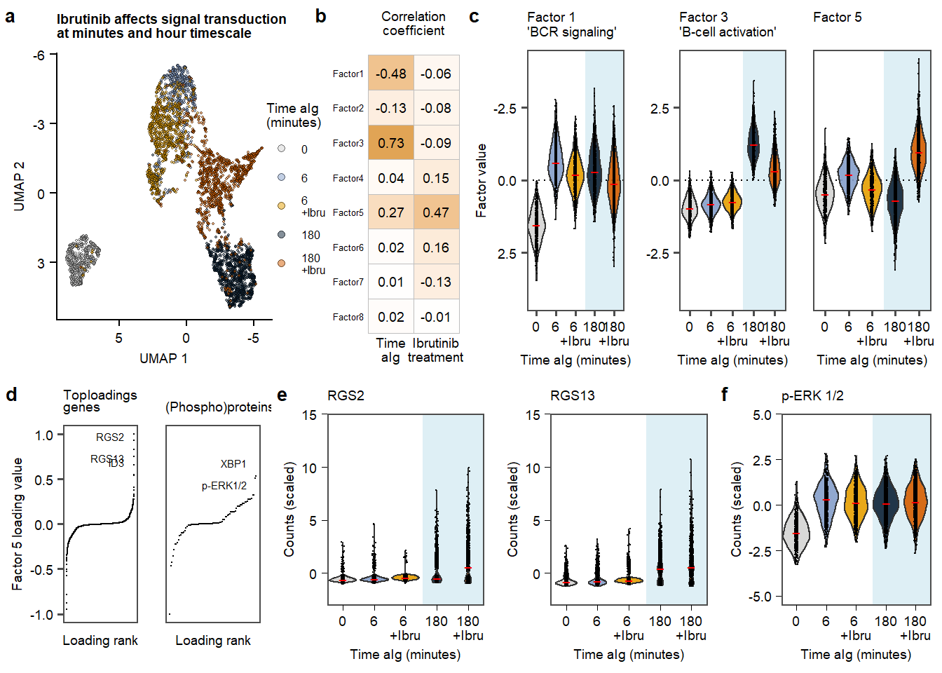
Figure 3. aIG stimultion in contect of Ibrutinib.

Supplementary MOFA model

## Variance per factor
plot.variance.perfactor.all <- plot_variance_explained(mofa, x="factor", y="view") +
    add.textsize +
    labs(title = "Variance explained by each factor per modality") 

## variance total
plot.variance.total <- plot_variance_explained(mofa, x="view", y="factor", plot_total = T)
plot.variance.total <- plot.variance.total[[2]] +
  add.textsize +
    labs(title = "Total \nvariance") +
  geom_text(aes(label=round(R2,1)), vjust=1.6, color="white", size=2.5)

## Significance correlation covariates
plot.heatmap.pval.covariates <- as.ggplot(correlate_factors_with_covariates(mofa, 
  covariates = c("time"),
  factors = 1:mofa@dimensions$K,
  fontsize = 7, 
  cluster_row = F,
  cluster_col = F
))+ 
  add.textsize +
  theme(axis.text.y=element_blank(),
        axis.text.x=element_blank(),
        plot.title = element_text(size=7, face = "plain"),
        )
## Factor values over time
plot.violin.factorall <- plot_factor(mofa, 
  factor = c(1:mofa@dimensions$K),
  color_by = "condition",
  dot_size = 0.2,      # change dot size
  dodge = T,           # dodge points with different colors
  legend = F,          # remove legend
  add_violin = T,      # add violin plots,
  violin_alpha = 0.9  # transparency of violin plots
) +   
  add.textsize +
  scale_color_manual(values=c(colorsibru, labels = c(labels), name = "Time aIg")) +
  scale_fill_manual(values=c(colorsibru, labels = c(labels), name = "Time aIg"))+
  labs(title = "Factor values per time-point of additional factors not correlating with time." ) +
  theme(axis.text.x=element_blank())

## Loadings factors stable protein

plot.rank.PROT.2.4to7 <- plot_weights(mofa, 
  view = "PROT", 
  factors = c(1:mofa@dimensions$K), 
  nfeatures = 3, 
  text_size = 1.5
) +   
  add.textsize +
  labs(title = "Top 3 Protein loadings per factor") +
  theme(axis.text.y=element_blank(),
        axis.ticks.y=element_blank()
)

## Loadings factors stable protein

plot.rank.RNA.2.4to7 <- plot_weights(mofa, 
  view = "RNA", 
  factors = c(1:mofa@dimensions$K), 
  nfeatures = 3, 
  text_size = 1.5
) +   
  add.textsize +
  labs(title = "Top 3 RNA loadings per factor") +
  theme(axis.text.y=element_blank(),
        axis.ticks.y=element_blank()
)

## correlation time and factors
plot.correlation.covariates <- correlate_factors_with_covariates(mofa, 
  covariates = c("time"),
  factors = mofa@dimensions$K:1,
  plot = "r"
)
plot.correlation.covariates <- ggcorrplot(plot.correlation.covariates, tl.col = "black", method = "square", lab = TRUE, ggtheme = theme_void, colors = c("#11304C", "white", "#11304C"), lab_size = 2.5) +
  add.textsize +
  labs(title = "Correlation of \nfactors with \ntime of treatment", y = "") +
  scale_y_discrete(labels = "") +
  coord_flip() +
  theme(axis.text.x=element_text(angle =0,hjust = 0.5), 
        axis.text.y=element_text(size = 5),
        legend.position="none",
        plot.title = element_text(hjust = 0.5))
Fig.3.suppl.mofa.row1 <- plot_grid(plot.variance.perfactor.all, plot.variance.total,NULL, plot.heatmap.pval.covariates, labels = c(panellabels[1:3]), label_size = 10, ncol = 4, rel_widths = c(1.35, 0.3,0.25,0.38))

Fig.3.suppl.mofa.row2 <- plot_grid(plot.violin.factorall,legend.umap, labels = panellabels[4], label_size = 10, ncol = 2, rel_widths = c(1,0.1))


Suppl_mofa <- plot_grid(Fig.3.suppl.mofa.row1, Fig.3.suppl.mofa.row2, plot.rank.PROT.2.4to7, plot.rank.RNA.2.4to7, labels = c("","", panellabels[5:6]),label_size = 10, ncol = 1, rel_heights = c(1.45,1,1.1,1.1))


ggsave(Suppl_mofa, filename = "output/paper_figures/Fig3.Suppl_MOFAibru.pdf", width = 183, height = 220, units = "mm",  dpi = 300, useDingbats = FALSE)
ggsave(Suppl_mofa, filename = "output/paper_figures/Fig3.Suppl_MOFAibru.png", width = 183, height = 220, units = "mm",  dpi = 300)

Suppl_mofa

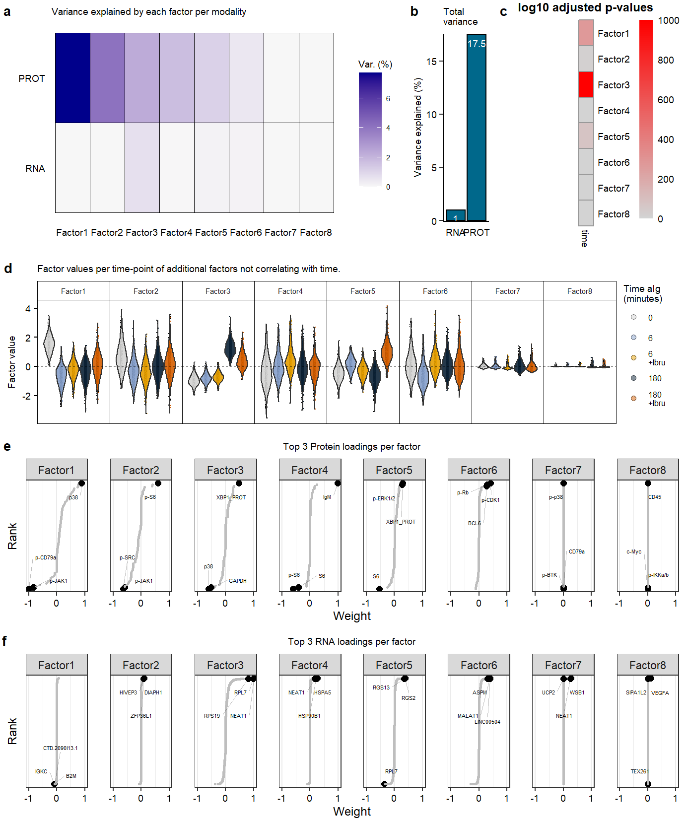
Supplementary Figure. MOFA model additional information

Enrichment genes factor 5 positve loadings (> 0.2).

# print positive enrichment
subset(enriched.go.bp.fct5.clusterdposneg@compareClusterResult, sign == "pos")
        Cluster  factor sign         ID
109 Factor5.pos Factor5  pos GO:0045744
110 Factor5.pos Factor5  pos GO:0008277
111 Factor5.pos Factor5  pos GO:0044557
112 Factor5.pos Factor5  pos GO:0007517
113 Factor5.pos Factor5  pos GO:0010958
114 Factor5.pos Factor5  pos GO:0015816
115 Factor5.pos Factor5  pos GO:0051956
116 Factor5.pos Factor5  pos GO:0061052
117 Factor5.pos Factor5  pos GO:1903789
118 Factor5.pos Factor5  pos GO:0060452
119 Factor5.pos Factor5  pos GO:1903960
120 Factor5.pos Factor5  pos GO:0045989
121 Factor5.pos Factor5  pos GO:0055119
122 Factor5.pos Factor5  pos GO:0086103
123 Factor5.pos Factor5  pos GO:0045986
124 Factor5.pos Factor5  pos GO:0060192
125 Factor5.pos Factor5  pos GO:0030903
126 Factor5.pos Factor5  pos GO:0030728
127 Factor5.pos Factor5  pos GO:2000726
128 Factor5.pos Factor5  pos GO:0032891
129 Factor5.pos Factor5  pos GO:0045662
130 Factor5.pos Factor5  pos GO:0061050
131 Factor5.pos Factor5  pos GO:0043951
132 Factor5.pos Factor5  pos GO:0051953
133 Factor5.pos Factor5  pos GO:1905208
134 Factor5.pos Factor5  pos GO:0045932
135 Factor5.pos Factor5  pos GO:0090075
136 Factor5.pos Factor5  pos GO:1903792
137 Factor5.pos Factor5  pos GO:0071875
138 Factor5.pos Factor5  pos GO:1903959
139 Factor5.pos Factor5  pos GO:0001975
140 Factor5.pos Factor5  pos GO:0042311
141 Factor5.pos Factor5  pos GO:0055022
142 Factor5.pos Factor5  pos GO:0061117
143 Factor5.pos Factor5  pos GO:0051955
144 Factor5.pos Factor5  pos GO:0010614
145 Factor5.pos Factor5  pos GO:0003298
146 Factor5.pos Factor5  pos GO:0003301
147 Factor5.pos Factor5  pos GO:0061049
148 Factor5.pos Factor5  pos GO:0014741
149 Factor5.pos Factor5  pos GO:0089718
150 Factor5.pos Factor5  pos GO:0046621
151 Factor5.pos Factor5  pos GO:0015804
152 Factor5.pos Factor5  pos GO:0045823
153 Factor5.pos Factor5  pos GO:0051154
154 Factor5.pos Factor5  pos GO:0043090
155 Factor5.pos Factor5  pos GO:0055026
156 Factor5.pos Factor5  pos GO:0014075
158 Factor5.pos Factor5  pos GO:0050873
159 Factor5.pos Factor5  pos GO:2000725
160 Factor5.pos Factor5  pos GO:0043949
162 Factor5.pos Factor5  pos GO:0045668
                                                                       Description
109            negative regulation of G protein-coupled receptor signaling pathway
110                     regulation of G protein-coupled receptor signaling pathway
111                                                    relaxation of smooth muscle
112                                                       muscle organ development
113                         regulation of amino acid import across plasma membrane
114                                                              glycine transport
115                                    negative regulation of amino acid transport
116 negative regulation of cell growth involved in cardiac muscle cell development
117                               regulation of amino acid transmembrane transport
118                              positive regulation of cardiac muscle contraction
119                           negative regulation of anion transmembrane transport
120                             positive regulation of striated muscle contraction
121                                                   relaxation of cardiac muscle
122         G protein-coupled receptor signaling pathway involved in heart process
123                               negative regulation of smooth muscle contraction
124                                         negative regulation of lipase activity
125                                                          notochord development
126                                                                      ovulation
127                     negative regulation of cardiac muscle cell differentiation
128                                  negative regulation of organic acid transport
129                                negative regulation of myoblast differentiation
130          regulation of cell growth involved in cardiac muscle cell development
131                                 negative regulation of cAMP-mediated signaling
132                                         negative regulation of amine transport
133                              negative regulation of cardiocyte differentiation
134                                      negative regulation of muscle contraction
135                                                           relaxation of muscle
136                                         negative regulation of anion transport
137                                          adrenergic receptor signaling pathway
138                                    regulation of anion transmembrane transport
139                                                        response to amphetamine
140                                                                   vasodilation
141                            negative regulation of cardiac muscle tissue growth
142                                            negative regulation of heart growth
143                                             regulation of amino acid transport
144                              negative regulation of cardiac muscle hypertrophy
145                                               physiological muscle hypertrophy
146                                       physiological cardiac muscle hypertrophy
147                        cell growth involved in cardiac muscle cell development
148                                      negative regulation of muscle hypertrophy
149                                       amino acid import across plasma membrane
150                                            negative regulation of organ growth
151                                                   neutral amino acid transport
152                                       positive regulation of heart contraction
153                    negative regulation of striated muscle cell differentiation
154                                                              amino acid import
155                       negative regulation of cardiac muscle tissue development
156                                                              response to amine
158                                                 brown fat cell differentiation
159                              regulation of cardiac muscle cell differentiation
160                                          regulation of cAMP-mediated signaling
162                              negative regulation of osteoblast differentiation
    GeneRatio   BgRatio       pvalue   p.adjust qvalue     geneID Count
109       2/4  53/18866 4.629425e-05 0.01083285     NA RGS13/RGS2     2
110       2/4 148/18866 3.629959e-04 0.04247052     NA RGS13/RGS2     2
111       1/4  10/18866 2.118699e-03 0.04724994     NA       RGS2     1
112       2/4 407/18866 2.706602e-03 0.04724994     NA   RGS2/ID3     2
113       1/4  13/18866 2.753652e-03 0.04724994     NA       RGS2     1
114       1/4  13/18866 2.753652e-03 0.04724994     NA       RGS2     1
115       1/4  13/18866 2.753652e-03 0.04724994     NA       RGS2     1
116       1/4  13/18866 2.753652e-03 0.04724994     NA       RGS2     1
117       1/4  13/18866 2.753652e-03 0.04724994     NA       RGS2     1
118       1/4  14/18866 2.965236e-03 0.04724994     NA       RGS2     1
119       1/4  15/18866 3.176786e-03 0.04724994     NA       RGS2     1
120       1/4  16/18866 3.388302e-03 0.04724994     NA       RGS2     1
121       1/4  16/18866 3.388302e-03 0.04724994     NA       RGS2     1
122       1/4  16/18866 3.388302e-03 0.04724994     NA       RGS2     1
123       1/4  17/18866 3.599785e-03 0.04724994     NA       RGS2     1
124       1/4  18/18866 3.811234e-03 0.04724994     NA       RGS2     1
125       1/4  20/18866 4.234030e-03 0.04724994     NA        ID3     1
126       1/4  21/18866 4.445378e-03 0.04724994     NA       RGS2     1
127       1/4  23/18866 4.867973e-03 0.04724994     NA       RGS2     1
128       1/4  24/18866 5.079220e-03 0.04724994     NA       RGS2     1
129       1/4  25/18866 5.290434e-03 0.04724994     NA        ID3     1
130       1/4  25/18866 5.290434e-03 0.04724994     NA       RGS2     1
131       1/4  26/18866 5.501614e-03 0.04724994     NA       RGS2     1
132       1/4  27/18866 5.712760e-03 0.04724994     NA       RGS2     1
133       1/4  27/18866 5.712760e-03 0.04724994     NA       RGS2     1
134       1/4  28/18866 5.923872e-03 0.04724994     NA       RGS2     1
135       1/4  31/18866 6.557008e-03 0.04724994     NA       RGS2     1
136       1/4  31/18866 6.557008e-03 0.04724994     NA       RGS2     1
137       1/4  32/18866 6.767986e-03 0.04724994     NA       RGS2     1
138       1/4  32/18866 6.767986e-03 0.04724994     NA       RGS2     1
139       1/4  33/18866 6.978931e-03 0.04724994     NA       RGS2     1
140       1/4  34/18866 7.189842e-03 0.04724994     NA       RGS2     1
141       1/4  34/18866 7.189842e-03 0.04724994     NA       RGS2     1
142       1/4  34/18866 7.189842e-03 0.04724994     NA       RGS2     1
143       1/4  36/18866 7.611563e-03 0.04724994     NA       RGS2     1
144       1/4  37/18866 7.822373e-03 0.04724994     NA       RGS2     1
145       1/4  38/18866 8.033149e-03 0.04724994     NA       RGS2     1
146       1/4  38/18866 8.033149e-03 0.04724994     NA       RGS2     1
147       1/4  38/18866 8.033149e-03 0.04724994     NA       RGS2     1
148       1/4  39/18866 8.243892e-03 0.04724994     NA       RGS2     1
149       1/4  41/18866 8.665277e-03 0.04724994     NA       RGS2     1
150       1/4  42/18866 8.875919e-03 0.04724994     NA       RGS2     1
151       1/4  43/18866 9.086528e-03 0.04724994     NA       RGS2     1
152       1/4  43/18866 9.086528e-03 0.04724994     NA       RGS2     1
153       1/4  43/18866 9.086528e-03 0.04724994     NA       RGS2     1
154       1/4  45/18866 9.507644e-03 0.04733593     NA       RGS2     1
155       1/4  45/18866 9.507644e-03 0.04733593     NA       RGS2     1
156       1/4  47/18866 9.928627e-03 0.04741426     NA       RGS2     1
158       1/4  50/18866 1.055985e-02 0.04845107     NA       RGS2     1
159       1/4  50/18866 1.055985e-02 0.04845107     NA       RGS2     1
160       1/4  53/18866 1.119077e-02 0.04849333     NA       RGS2     1
162       1/4  53/18866 1.119077e-02 0.04849333     NA        ID3     1

Supplementary violins

Suppl.row1 <- plot_grid(`plot.violin.prot.p-PLC-y2Y759`, `plot.violin.prot.p-BLNK`,`plot.violin.prot.p-CD79a`,`plot.violin.prot.p-Syk`,`plot.violin.prot.p-JAK1`,labels = panellabels[1], label_size = 10, ncol = 5, rel_widths = c(1,1,1,1,1))

Suppl.row2 <- plot_grid(plot.violin.RNA.NEAT1, plot.violin.RNA.NPM1, plot.violin.RNA.BTF3,labels = panellabels[2], label_size = 10, ncol = 5, rel_widths = c(1,1,1,1,1))

Suppl_ibru_protsgenes <- plot_grid(Suppl.row1, Suppl.row2,label_size = 10, ncol = 1, rel_heights = c(1,1))

ggsave(Suppl_ibru_protsgenes, filename = "output/paper_figures/Fig3.suppl.violinsibru.pdf", width = 183, height = 122, units = "mm",  dpi = 300, useDingbats = FALSE)
ggsave(Suppl_ibru_protsgenes, filename = "output/paper_figures/Fig3.suppl.violinsibru.png", width = 183, height = 122, units = "mm",  dpi = 300)

Suppl_ibru_protsgenes

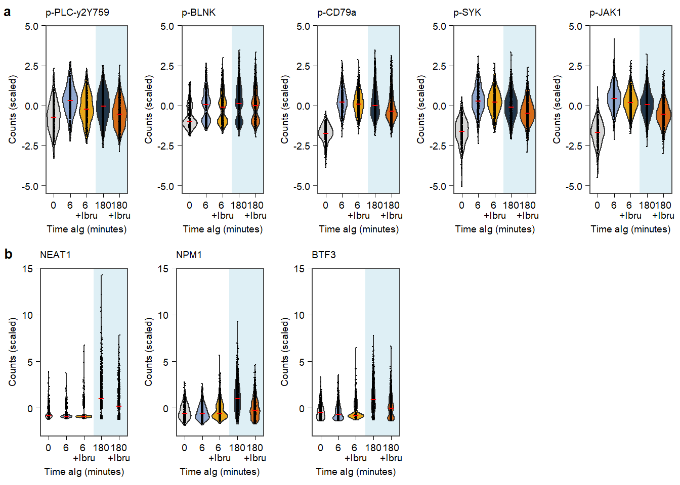
Supplementary Figure. Violin plots of highlighted phopho-proteins & genes


sessionInfo()
R version 4.0.3 (2020-10-10)
Platform: x86_64-w64-mingw32/x64 (64-bit)
Running under: Windows 10 x64 (build 19042)

Matrix products: default

locale:
[1] LC_COLLATE=English_Netherlands.1252  LC_CTYPE=English_Netherlands.1252   
[3] LC_MONETARY=English_Netherlands.1252 LC_NUMERIC=C                        
[5] LC_TIME=English_Netherlands.1252    

attached base packages:
 [1] parallel  stats4    grid      stats     graphics  grDevices utils    
 [8] datasets  methods   base     

other attached packages:
 [1] png_0.1-7                   forcats_0.5.1              
 [3] clusterProfiler_3.18.1      clusterProfiler.dplyr_0.0.2
 [5] enrichplot_1.10.2           org.Hs.eg.db_3.12.0        
 [7] AnnotationDbi_1.52.0        IRanges_2.24.1             
 [9] S4Vectors_0.28.1            Biobase_2.50.0             
[11] BiocGenerics_0.36.0         ggridges_0.5.3             
[13] cowplot_1.1.1               ggtext_0.1.1               
[15] ggplotify_0.0.5             ggcorrplot_0.1.3           
[17] ggrepel_0.9.1               ggpubr_0.4.0               
[19] scico_1.2.0                 MOFA2_1.1.17               
[21] extrafont_0.17              patchwork_1.1.1            
[23] RColorBrewer_1.1-2          viridis_0.5.1              
[25] viridisLite_0.3.0           ggsci_2.9                  
[27] sctransform_0.3.2           ggthemes_4.2.4             
[29] matrixStats_0.57.0          kableExtra_1.3.1           
[31] gridExtra_2.3               SeuratObject_4.0.0         
[33] Seurat_4.0.0                ggplot2_3.3.3              
[35] scales_1.1.1                tidyr_1.1.2                
[37] dplyr_1.0.3                 stringr_1.4.0              
[39] workflowr_1.6.2            

loaded via a namespace (and not attached):
  [1] rappdirs_0.3.2       scattermore_0.7      bit64_4.0.5         
  [4] knitr_1.31           irlba_2.3.3          DelayedArray_0.16.1 
  [7] data.table_1.13.6    rpart_4.1-15         generics_0.1.0      
 [10] RSQLite_2.2.3        shadowtext_0.0.7     RANN_2.6.1          
 [13] future_1.21.0        bit_4.0.4            spatstat.data_2.1-0 
 [16] webshot_0.5.2        xml2_1.3.2           httpuv_1.5.5        
 [19] assertthat_0.2.1     xfun_0.23            hms_1.0.0           
 [22] evaluate_0.14        promises_1.1.1       readxl_1.3.1        
 [25] tmvnsim_1.0-2        igraph_1.2.6         DBI_1.1.1           
 [28] htmlwidgets_1.5.3    purrr_0.3.4          ellipsis_0.3.1      
 [31] corrplot_0.84        backports_1.2.1      markdown_1.1        
 [34] deldir_0.2-10        MatrixGenerics_1.2.0 vctrs_0.3.6         
 [37] ROCR_1.0-11          abind_1.4-5          cachem_1.0.1        
 [40] withr_2.4.1          ggforce_0.3.2        mnormt_2.0.2        
 [43] goftest_1.2-2        cluster_2.1.0        DOSE_3.16.0         
 [46] lazyeval_0.2.2       crayon_1.3.4         basilisk.utils_1.2.1
 [49] pkgconfig_2.0.3      labeling_0.4.2       tweenr_1.0.1        
 [52] nlme_3.1-149         rlang_0.4.10         globals_0.14.0      
 [55] lifecycle_0.2.0      miniUI_0.1.1.1       downloader_0.4      
 [58] filelock_1.0.2       extrafontdb_1.0      cellranger_1.1.0    
 [61] rprojroot_2.0.2      polyclip_1.10-0      lmtest_0.9-38       
 [64] Matrix_1.2-18        carData_3.0-4        Rhdf5lib_1.12.1     
 [67] zoo_1.8-8            whisker_0.4          pheatmap_1.0.12     
 [70] KernSmooth_2.23-17   rhdf5filters_1.2.0   blob_1.2.1          
 [73] qvalue_2.22.0        parallelly_1.23.0    rstatix_0.6.0       
 [76] gridGraphics_0.5-1   ggsignif_0.6.0       memoise_2.0.0       
 [79] magrittr_2.0.1       plyr_1.8.6           ica_1.0-2           
 [82] compiler_4.0.3       scatterpie_0.1.5     fitdistrplus_1.1-3  
 [85] listenv_0.8.0        pbapply_1.4-3        MASS_7.3-53         
 [88] mgcv_1.8-33          tidyselect_1.1.0     stringi_1.5.3       
 [91] highr_0.8            yaml_2.2.1           GOSemSim_2.16.1     
 [94] fastmatch_1.1-0      tools_4.0.3          future.apply_1.7.0  
 [97] rio_0.5.16           rstudioapi_0.13      foreign_0.8-80      
[100] git2r_0.28.0         farver_2.0.3         Rtsne_0.15          
[103] ggraph_2.0.5         digest_0.6.27        rvcheck_0.1.8       
[106] BiocManager_1.30.10  shiny_1.6.0          Rcpp_1.0.6          
[109] gridtext_0.1.4       car_3.0-10           broom_0.7.3         
[112] later_1.1.0.1        RcppAnnoy_0.0.18     httr_1.4.2          
[115] psych_2.0.12         colorspace_2.0-0     rvest_0.3.6         
[118] fs_1.5.0             tensor_1.5           reticulate_1.18     
[121] splines_4.0.3        uwot_0.1.10          spatstat.utils_2.1-0
[124] graphlayouts_0.7.1   basilisk_1.2.1       plotly_4.9.3        
[127] xtable_1.8-4         jsonlite_1.7.2       spatstat_1.64-1     
[130] tidygraph_1.2.0      R6_2.5.0             pillar_1.4.7        
[133] htmltools_0.5.1.1    mime_0.9             glue_1.4.2          
[136] fastmap_1.1.0        BiocParallel_1.24.1  codetools_0.2-16    
[139] fgsea_1.16.0         lattice_0.20-41      tibble_3.0.5        
[142] curl_4.3             leiden_0.3.7         zip_2.1.1           
[145] GO.db_3.12.1         openxlsx_4.2.3       Rttf2pt1_1.3.8      
[148] survival_3.2-7       rmarkdown_2.6        munsell_0.5.0       
[151] DO.db_2.9            rhdf5_2.34.0         HDF5Array_1.18.0    
[154] haven_2.3.1          reshape2_1.4.4       gtable_0.3.0