Orange County, CA COVID-19 Situation Report Start Date - End Date
Last updated: 2020-08-26
Checks: 6 1
Knit directory: uci_covid_modeling/
This reproducible R Markdown analysis was created with workflowr (version 1.6.2). The Checks tab describes the reproducibility checks that were applied when the results were created. The Past versions tab lists the development history.
The R Markdown file has unstaged changes. To know which version of the R Markdown file created these results, you’ll want to first commit it to the Git repo. If you’re still working on the analysis, you can ignore this warning. When you’re finished, you can run wflow_publish to commit the R Markdown file and build the HTML.
Great job! The global environment was empty. Objects defined in the global environment can affect the analysis in your R Markdown file in unknown ways. For reproduciblity it’s best to always run the code in an empty environment.
The command set.seed(20200727) was run prior to running the code in the R Markdown file. Setting a seed ensures that any results that rely on randomness, e.g. subsampling or permutations, are reproducible.
Great job! Recording the operating system, R version, and package versions is critical for reproducibility.
Nice! There were no cached chunks for this analysis, so you can be confident that you successfully produced the results during this run.
Great job! Using relative paths to the files within your workflowr project makes it easier to run your code on other machines.
Great! You are using Git for version control. Tracking code development and connecting the code version to the results is critical for reproducibility.
The results in this page were generated with repository version 8d4a8dc. See the Past versions tab to see a history of the changes made to the R Markdown and HTML files.
Note that you need to be careful to ensure that all relevant files for the analysis have been committed to Git prior to generating the results (you can use wflow_publish or wflow_git_commit). workflowr only checks the R Markdown file, but you know if there are other scripts or data files that it depends on. Below is the status of the Git repository when the results were generated:
Ignored files:
    Ignored:    .Rhistory
    Ignored:    .Rproj.user/

Untracked files:
    Untracked:  analysis/jun20_jul25.Rmd
    Untracked:  analysis/style.css

Unstaged changes:
    Modified:   analysis/_site.yml
    Modified:   analysis/index.Rmd
    Modified:   uci_covid_modeling.Rproj
Note that any generated files, e.g. HTML, png, CSS, etc., are not included in this status report because it is ok for generated content to have uncommitted changes.
These are the previous versions of the repository in which changes were made to the R Markdown (analysis/index.Rmd) and HTML (docs/index.html) files. If you’ve configured a remote Git repository (see ?wflow_git_remote), click on the hyperlinks in the table below to view the files as they were in that past version.
| File | Version | Author | Date | Message |
|---|---|---|---|---|
| Rmd | 64adfeb | igoldsteinh | 2020-08-20 | cleaning up helper functions and index |
| Rmd | 8abe830 | igoldsteinh | 2020-08-06 | fixed figure length, updated, tried a readme |
| html | 8abe830 | igoldsteinh | 2020-08-06 | fixed figure length, updated, tried a readme |
| Rmd | 99d68f7 | igoldsteinh | 2020-07-29 | bare bones report |
| html | 99d68f7 | igoldsteinh | 2020-07-29 | bare bones report |
| Rmd | 792b89a | vnminin | 2020-07-27 | Start workflowr project. |
Introduction
The goal of this report is to inform interested parties about dynamics of SARS-CoV-2 spread in Orange County, CA and to predict (if feasible) the outbreak epidemic trajectory. Our approach is based on fitting a mechanistic model of SARS-CoV-2 spread to multiple sources of surveillance data. More specifically, we use daily numbers of new cases and deaths, while taking into account changes in the total number of tests reported on each day.
Executive summary
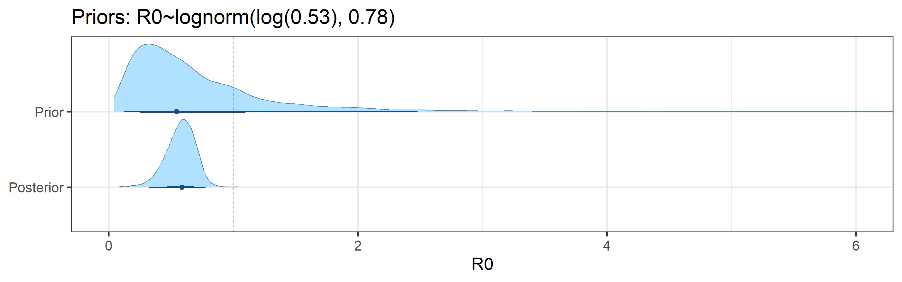
- 95% Bayesian credible interval for the basic reproductive number \(R_0\) is (0.37, 0.8).
- 95% Bayesian credible interval for the total number of infections that had occurred between June 20, 2020 and July 25, 2020 is (13,000, 110,000). The number of reported cases in this period was 23,000.
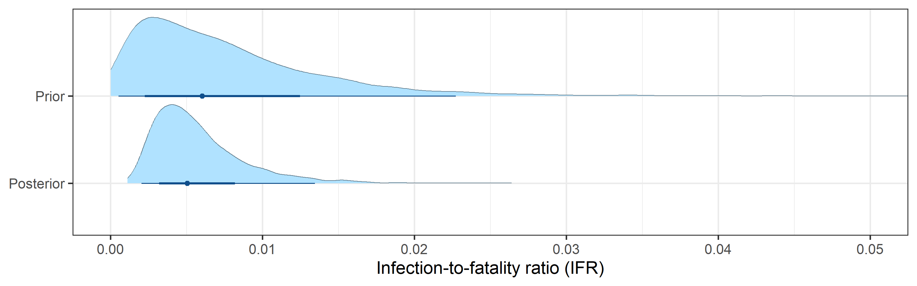
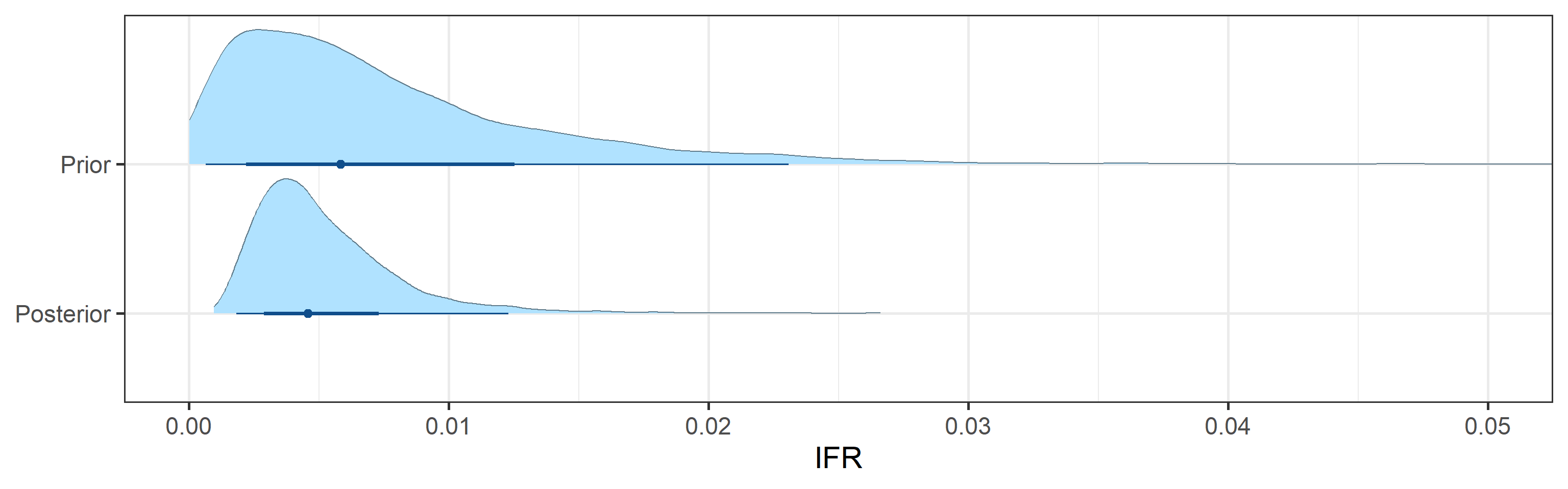
- 95% Bayesian credible interval for the infection-to-fatality ratio (IFR), defined as a fraction of deaths among the total number of infections, is (0.002, 0.013).
Since we rely on a mechanistic model, it is important to acknowledge limitations of this model. We will try to be transparent about our assumptions in the hope to receive feedback about their realism. So if something does not look right to you, please get in touch with us to help us improve our model.
Model inputs
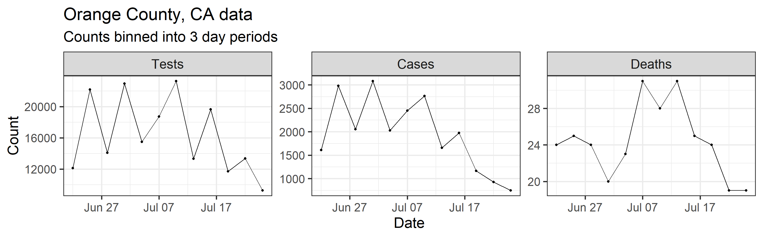
Our method takes three time series as input: daily new tests, case counts, and deaths. However, we find daily resolution to be too noisy due to delay in testing reports, weekend effect, etc. So we aggregated/binned the three types of counts in 3 day intervals. These aggregated time series are shown below.
Model structure
We assume that all individuals in Orange County, CA can be split into 6 compartments: S = susceptible individuals, E = infected, but not yet infectious individuals, \(\text{I}_\text{e}\) = individuals at early stages of infection, \(\text{I}_\text{p}\) = individuals at progressed stages of infection (assumed 20% less infectious than individuals at the early infection stage), R = recovered individuals, D = individuals who died due to COVID-19. Possible progressions of an individual through the above compartments are depicted in the diagram below.

Mathematically, we assume that dynamics of the proportions of individuals in each compartment follow a set of ordinary differential equations corresponding to the above diagram. These equations are controlled by the following parameters:
- Basic reproductive number (\(R_0\))
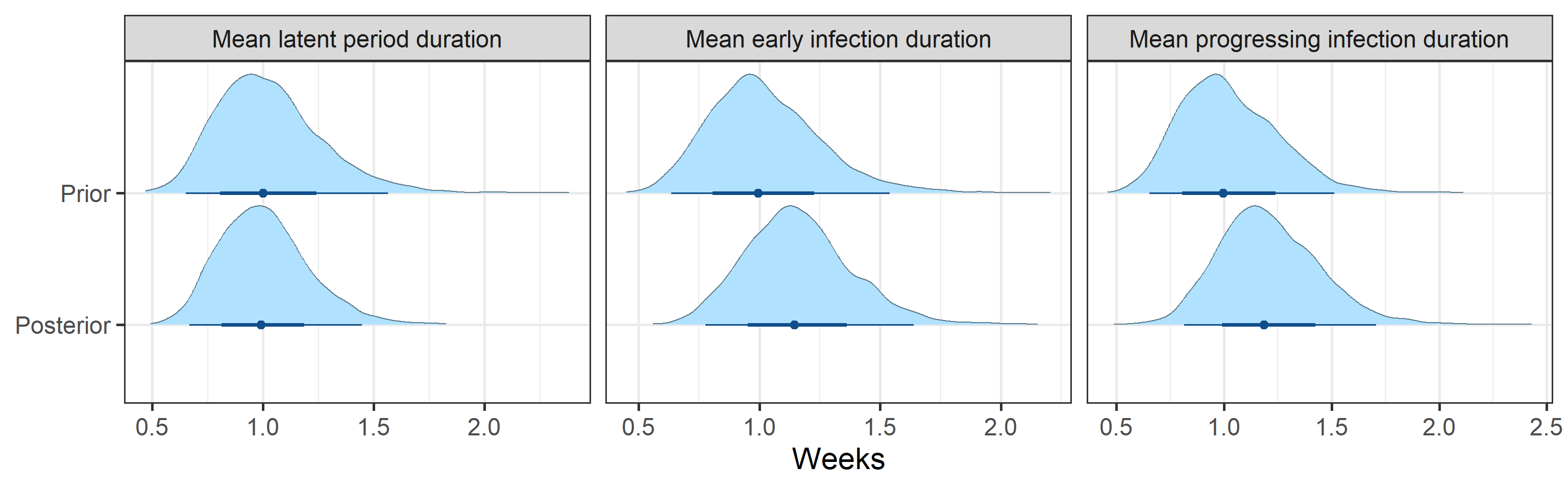
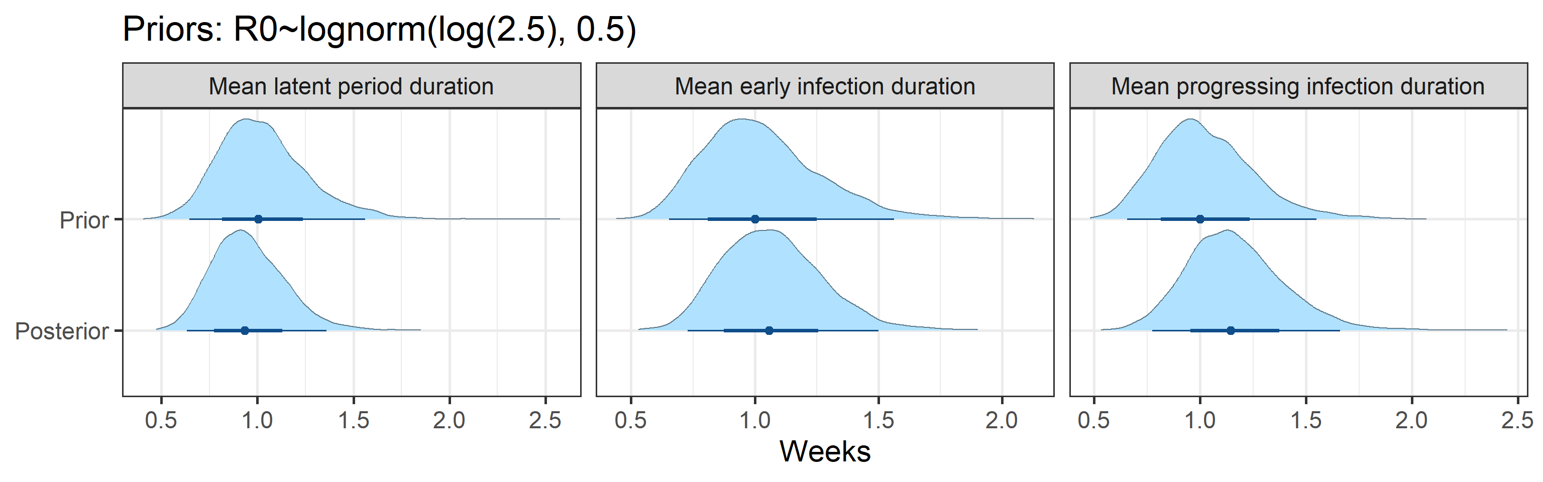
- mean duration of the latent period
- mean duration of the early infection period
- mean duration of the progressed infection period
- probability of transitioning from progressed infection to death, rather than to recovery (i.e., IFR)
We fit this model to data by assuming that case counts are noisy realizations of the actual number of individuals progressing from \(\text{I}_\text{e}\) compartment to \(\text{I}_\text{p}\) compartment. Similarly we assume that observed deaths are noisy realizations of the actual number of individuals progressing from \(\text{I}_\text{p}\) compartment to \(\text{D}\) compartment. A priori, we assume that death counts are significantly less noisy than case counts. We use a Bayesian estimation framework, which means that all estimated quantities receive credible intervals (e.g., 80% or 95% credible intervals). Width of these credible intervals encode the amount of uncertainty that we have in the estimated quantities.
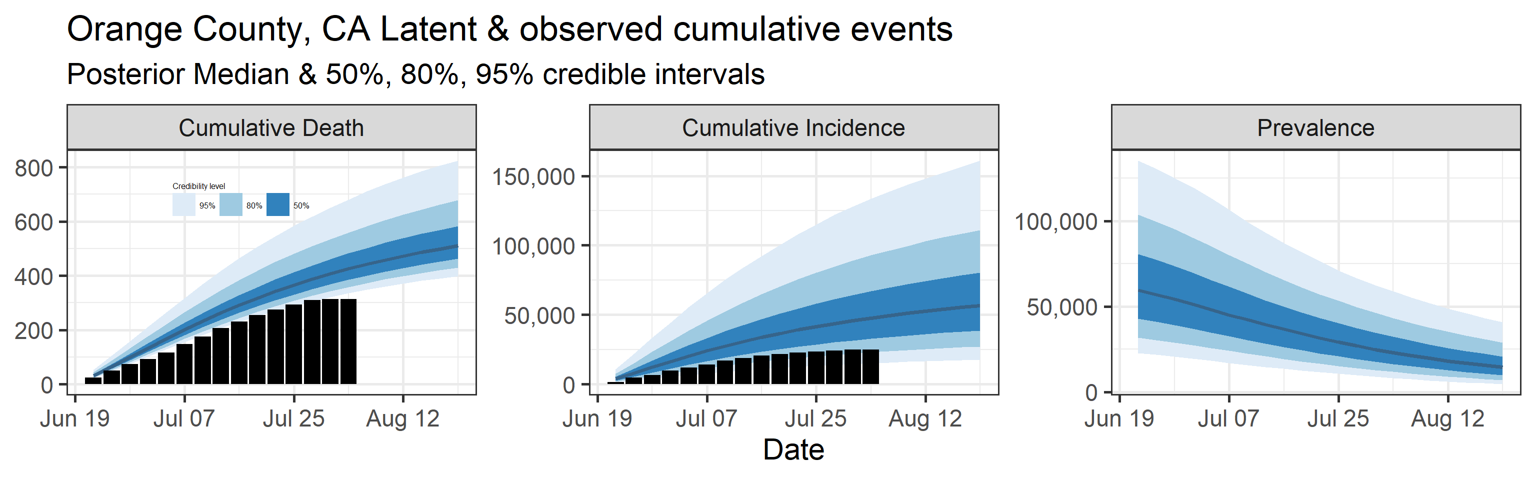
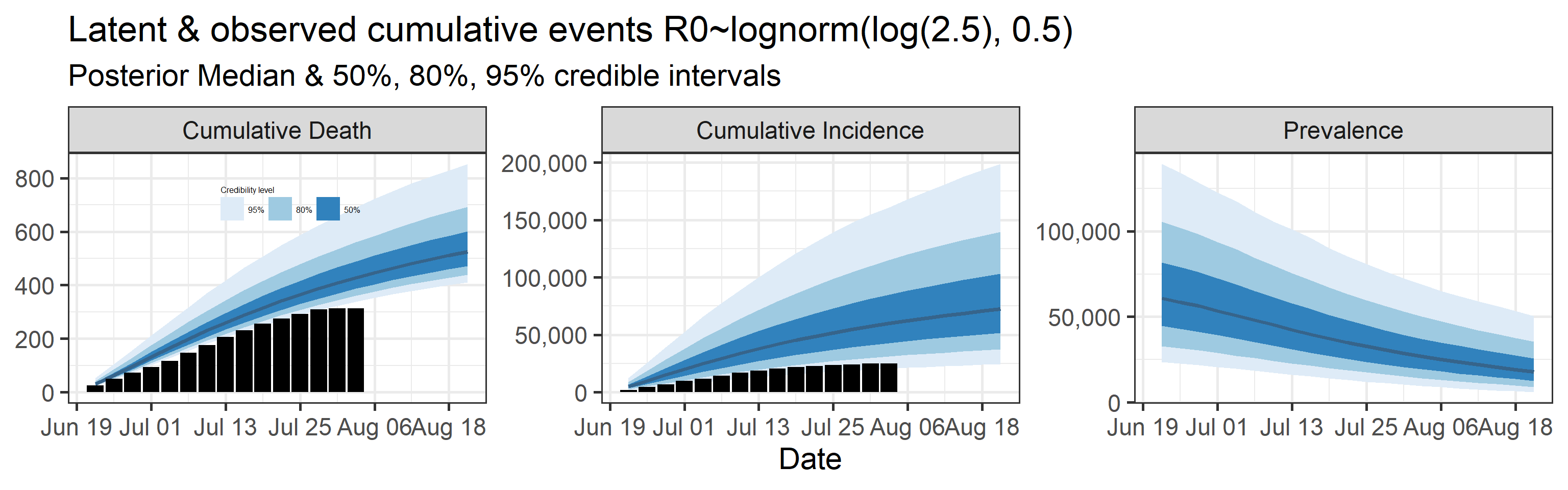
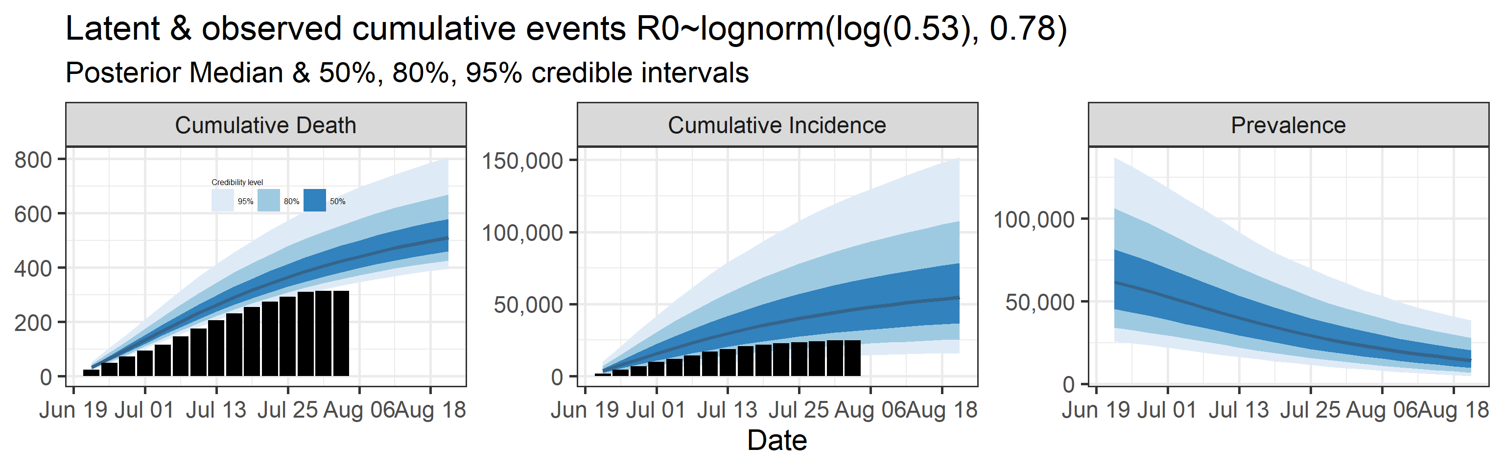
Latent cumulative deaths, cumulative incidence, and prevalence
We report estimated trajectories of latent cumulative deaths, incidence (i.e., total infections and deaths that have occurred by some prespecified time point), and prevalence . These trajectories represent our estimation of accumulation of unobserved/hidden number of infections and deaths in the Orange County population. We also project these three trajectories 4 weeks into the future.
The main takeaways are:
- Cases underestimate the total number of infections by a factor that ranges with 95% probability between 0.57 and 4.9. This means that we estimate that the total number of infections between June 20, 2020 and July 25, 2020 is between 13,000 and 110,000. The number of reported cases in this period was 23,000.
- 95% Bayesian credible interval of death underreporting factor is (0.52, 0.97).
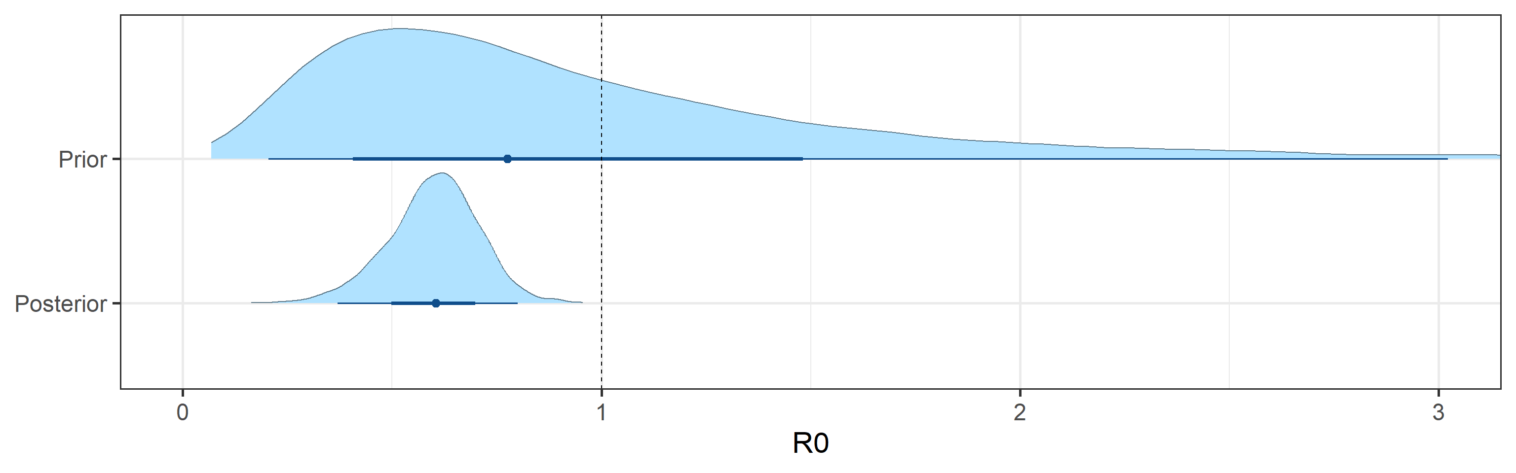
Prior and posterior distributions of model parameters
Next we report prior and posterior distributions of key model parameters. Prior distributions represent our beliefs about these parameters before seeing/analyzing data. Posterior distributions encode our updated beliefs after seeing/analyzing data.
The main takeaways are:
- 95% Bayesian credible interval for the basic reproductive number \(R_0\) is (0.37, 0.8). The posterior probability that \(R_0\) is above 1.0 is 0%.
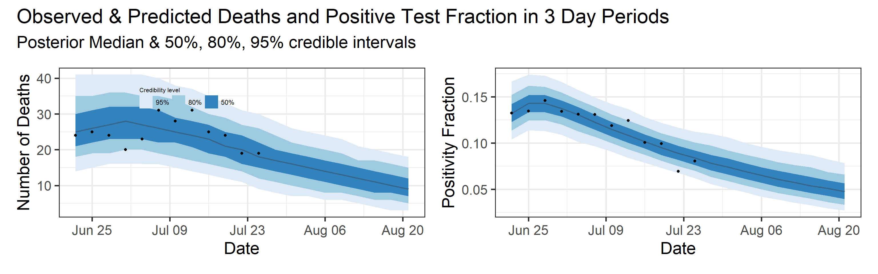
Reported deaths and positive test rate forecast
We report predictive distribution of observed deaths and positive test rate during the observation interval (blue shaded area with black dots in the plot below). In addition, we show a four week ahead forecast for both quantities. Our forecast assumes that interventions (physical distancing orders, mask recommendations, etc.) stay at the status quo, and that there are 2100 tests in each three day interval in the future. We plan to archive our forecasts and retrospectively measure their predictive ability/skill.
Modeling limitations
- Some model parameters are not well identified, so we rely on scientifically sound prior information (please check our assumptions and help us improve our priors!). We will include sensitivity to prior analyses as an appendix in future reports.
- The model assumes a well mixed population with no geographic or age structure.
- Basic reproductive number (\(R_0\)) is constant. However, implementation of physical distancing and school closures should gradually reduce it. Similarly, relaxing current physical distancing measures will start increasing \(R_0\).
Planned model extensions
- We plan to add H = hospitalized and ICU compartments to the model. This extension will allow us to inform the model with hospitalization and occupied ICU beds time series, in addition to already used test, case, and death counts. Equally importantly, we will be able to forecast hospital and ICU occupancy.
- We will allow \(R_0\) to vary with time and will attempt to estimate its changes non-parameterically.
- We would like to add age structure into the model. This is not a high priority at the moment, because we suspect we don’t have enough data to estimate additional parameters that will need to be added to the model.
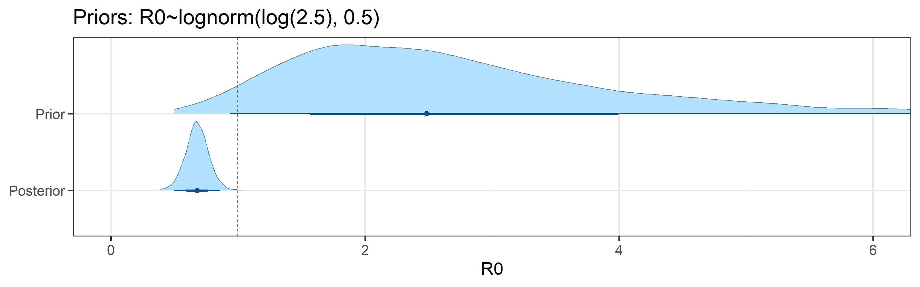
Appendix
Sensitivity to Prior for \(R_0\)
We examine how sensitive our conclusions about \(R_0\) to our prior assumptions by repeating estimation of all model parameters under different priors for this parameter. The priors are listed in the titles of the figures. Although the prior distribution of \(R_0\) does have some effect on its posterior (as it should), the our results and conclusions are not too sensitive to a particular specification of this prior.
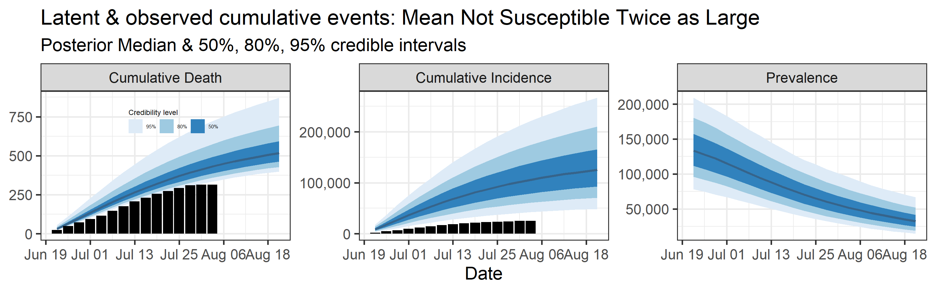
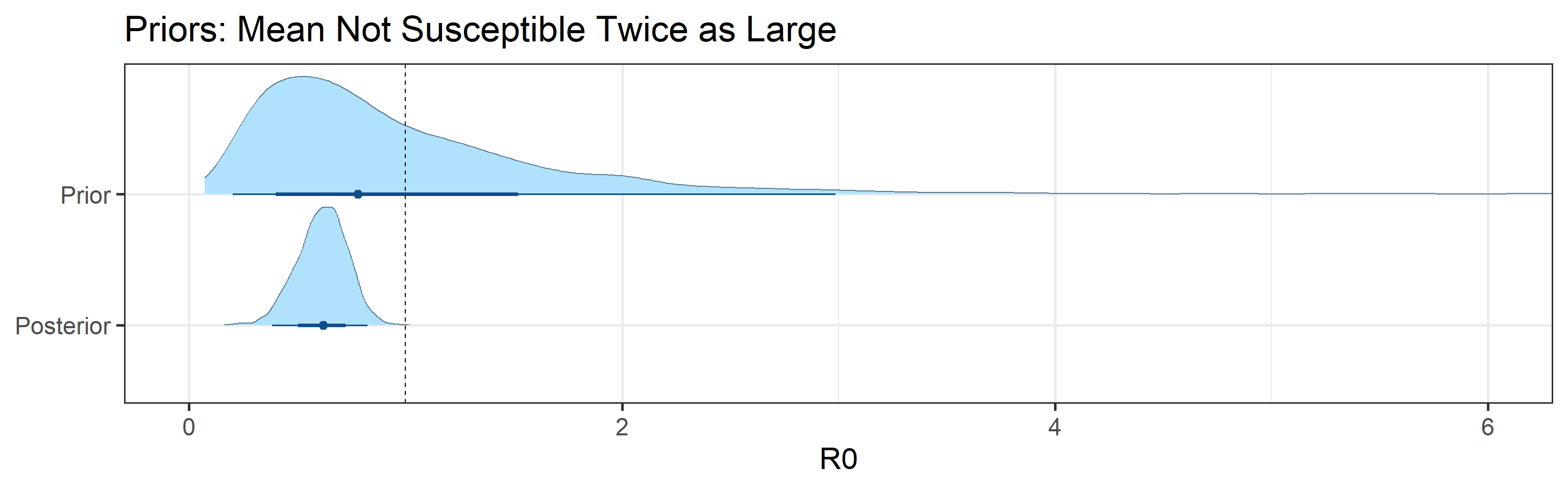
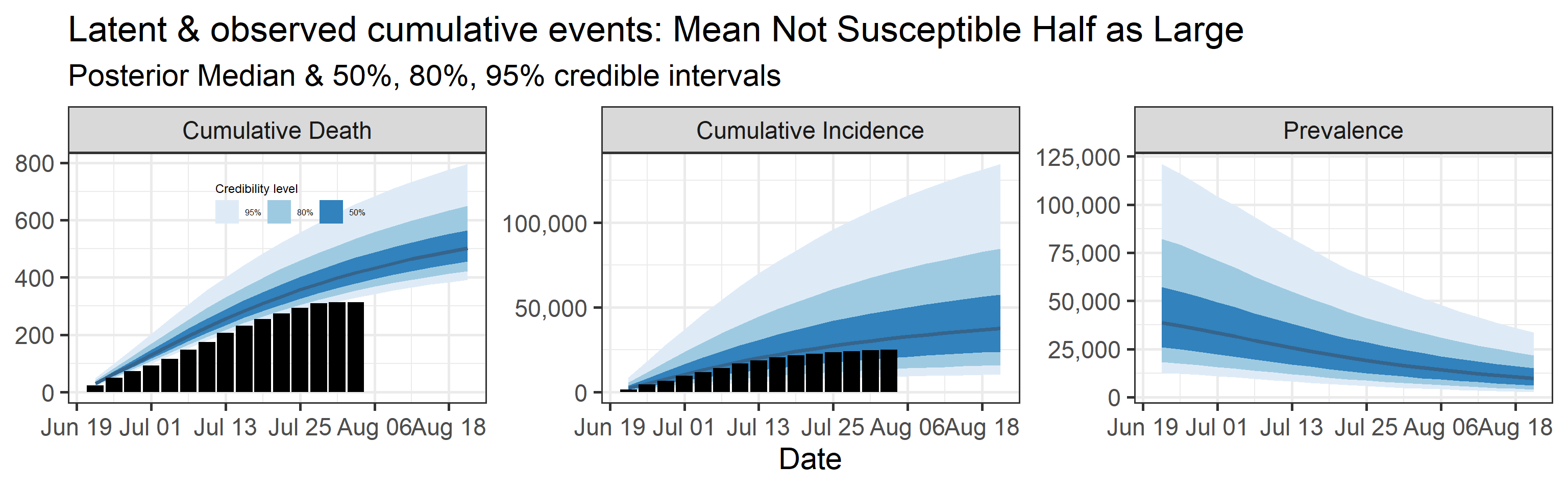
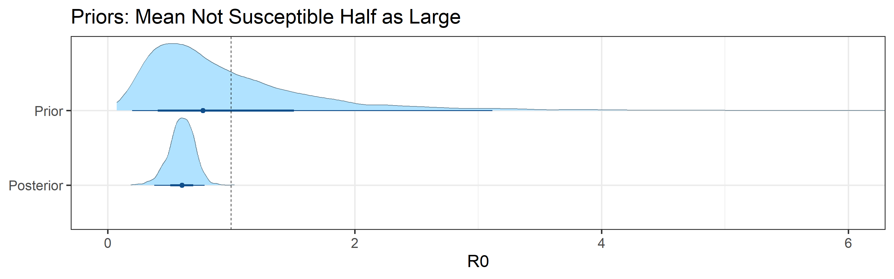
Sensitivity to prior for fraction not susceptible
We examine how sensitive our conclusions about \(R_0\) to our prior assumptions by repeating estimation of all model parameters under different priors for the parameter controlling how many people are not susceptible initially. This prior changes depending on the time period, so we adjust by changing the prior mean to be twice as large or one half as large as the default prior. As we would expect, changing this prior changes the number of people we estimate will become infected or are currently infectious. However, it seems to have little impact on the posterior of \(R_0\).
R version 4.0.2 (2020-06-22)
Platform: x86_64-w64-mingw32/x64 (64-bit)
Running under: Windows 10 x64 (build 18362)

Matrix products: default

locale:
[1] LC_COLLATE=English_United States.1252
[2] LC_CTYPE=English_United States.1252
[3] LC_MONETARY=English_United States.1252
[4] LC_NUMERIC=C
[5] LC_TIME=English_United States.1252

attached base packages:
[1] stats     graphics  grDevices utils     datasets  methods   base

other attached packages:
 [1] patchwork_1.0.1 scales_1.1.1    tidybayes_2.1.1 forcats_0.5.0
 [5] stringr_1.4.0   dplyr_1.0.0     purrr_0.3.4     readr_1.3.1
 [9] tidyr_1.1.0     tibble_3.0.3    ggplot2_3.3.2   tidyverse_1.3.0
[13] here_0.1        lubridate_1.7.9 workflowr_1.6.2

loaded via a namespace (and not attached):
 [1] matrixStats_0.56.0   fs_1.4.2             RColorBrewer_1.1-2
 [4] httr_1.4.1           rprojroot_1.3-2      rstan_2.21.2
 [7] tools_4.0.2          backports_1.1.8      utf8_1.1.4
[10] R6_2.4.1             DBI_1.1.0            colorspace_1.4-1
[13] ggdist_2.2.0         withr_2.2.0          gridExtra_2.3
[16] tidyselect_1.1.0     prettyunits_1.1.1    processx_3.4.3
[19] curl_4.3             compiler_4.0.2       git2r_0.27.1
[22] cli_2.0.2            rvest_0.3.5          arrayhelpers_1.1-0
[25] xml2_1.3.2           labeling_0.3         callr_3.4.3
[28] digest_0.6.25        StanHeaders_2.21.0-5 rmarkdown_2.3
[31] pkgconfig_2.0.3      htmltools_0.5.0      dbplyr_1.4.4
[34] rlang_0.4.7          readxl_1.3.1         rstudioapi_0.11
[37] farver_2.0.3         generics_0.0.2       svUnit_1.0.3
[40] jsonlite_1.7.0       distributional_0.1.0 inline_0.3.15
[43] magrittr_1.5         loo_2.3.1            Rcpp_1.0.5
[46] munsell_0.5.0        fansi_0.4.1          lifecycle_0.2.0
[49] stringi_1.4.6        whisker_0.4          yaml_2.2.1
[52] pkgbuild_1.1.0       plyr_1.8.6           grid_4.0.2
[55] blob_1.2.1           parallel_4.0.2       promises_1.1.1
[58] crayon_1.3.4         lattice_0.20-41      haven_2.3.1
[61] hms_0.5.3            knitr_1.29           ps_1.3.3
[64] pillar_1.4.6         codetools_0.2-16     stats4_4.0.2
[67] reprex_0.3.0         glue_1.4.1           evaluate_0.14
[70] V8_3.2.0             RcppParallel_5.0.2   modelr_0.1.8
[73] vctrs_0.3.2          httpuv_1.5.4         cellranger_1.1.0
[76] gtable_0.3.0         assertthat_0.2.1     xfun_0.15
[79] broom_0.7.0          coda_0.19-3          later_1.1.0.1
[82] ellipsis_0.3.1