evaluation
wiesehahn
2020-07-23
Last updated: 2020-08-04
Checks: 6 1
Knit directory: baumarten/analysis/
This reproducible R Markdown analysis was created with workflowr (version 1.6.2). The Checks tab describes the reproducibility checks that were applied when the results were created. The Past versions tab lists the development history.
The R Markdown file has unstaged changes. To know which version of the R Markdown file created these results, you’ll want to first commit it to the Git repo. If you’re still working on the analysis, you can ignore this warning. When you’re finished, you can run wflow_publish to commit the R Markdown file and build the HTML.
Great job! The global environment was empty. Objects defined in the global environment can affect the analysis in your R Markdown file in unknown ways. For reproduciblity it’s best to always run the code in an empty environment.
The command set.seed(20200723) was run prior to running the code in the R Markdown file. Setting a seed ensures that any results that rely on randomness, e.g. subsampling or permutations, are reproducible.
Great job! Recording the operating system, R version, and package versions is critical for reproducibility.
Nice! There were no cached chunks for this analysis, so you can be confident that you successfully produced the results during this run.
Great job! Using relative paths to the files within your workflowr project makes it easier to run your code on other machines.
Great! You are using Git for version control. Tracking code development and connecting the code version to the results is critical for reproducibility.
The results in this page were generated with repository version f261bcc. See the Past versions tab to see a history of the changes made to the R Markdown and HTML files.
Note that you need to be careful to ensure that all relevant files for the analysis have been committed to Git prior to generating the results (you can use wflow_publish or wflow_git_commit). workflowr only checks the R Markdown file, but you know if there are other scripts or data files that it depends on. Below is the status of the Git repository when the results were generated:
Ignored files:
    Ignored:    .Rhistory
    Ignored:    .Rproj.user/
    Ignored:    analysis/.Rhistory
    Ignored:    analysis/figure/

Untracked files:
    Untracked:  analysis/classification.Rmd
    Untracked:  analysis/preprocessing.Rmd
    Untracked:  data/sen2/

Unstaged changes:
    Modified:   .gitignore
    Modified:   analysis/evaluation.Rmd
    Modified:   code/workflow_project_setup.R
Note that any generated files, e.g. HTML, png, CSS, etc., are not included in this status report because it is ok for generated content to have uncommitted changes.
These are the previous versions of the repository in which changes were made to the R Markdown (analysis/evaluation.Rmd) and HTML (docs/evaluation.html) files. If you’ve configured a remote Git repository (see ?wflow_git_remote), click on the hyperlinks in the table below to view the files as they were in that past version.
| File | Version | Author | Date | Message |
|---|---|---|---|---|
| Rmd | c7df603 | wiesehahn | 2020-07-28 | general additions |
| html | c7df603 | wiesehahn | 2020-07-28 | general additions |
| html | f400426 | wiesehahn | 2020-07-23 | init |
| Rmd | 369d039 | wiesehahn | 2020-07-23 | wflow_git_commit(all = T) |
| Rmd | 27a9ab6 | wiesehahn | 2020-07-23 | wflow_git_commit(“evaluation.Rmd”) |
Introduction
Validation Steps
(classification steps and validation possibilities)
Input Data
- Choice of satellite imagery (date, quality)
- Preprocessing steps (atmospheric, topographic, … correction)
- Image masking (clouds, cloud shadows, nodata)
Reference Data
- Choice of reference data (distribution)
- Label reference data
- Extraction of input data for reference areas
- Splitting in train and test data sets
Build Classification Model
- Choice of classification features
- Choice of model hyperparameters
Apply Classification Model
- Input data classification
- Class probability calculation
Postprocessing
- Apply filter (Minimal Mapping Unit, Focal filter)
- Integration of class probabilities
Accuracy Assessment
- Calculate accuracy metrics from validation data
Reference Data
The reference data was sampled in three project areas (Harz, Heide, Solling).Reference data sampling locations
Number of reference data polygons by tree species
Number of reference data polygons by site
Number of reference data polygons by tree species and site
Classification
Study sites
Solling
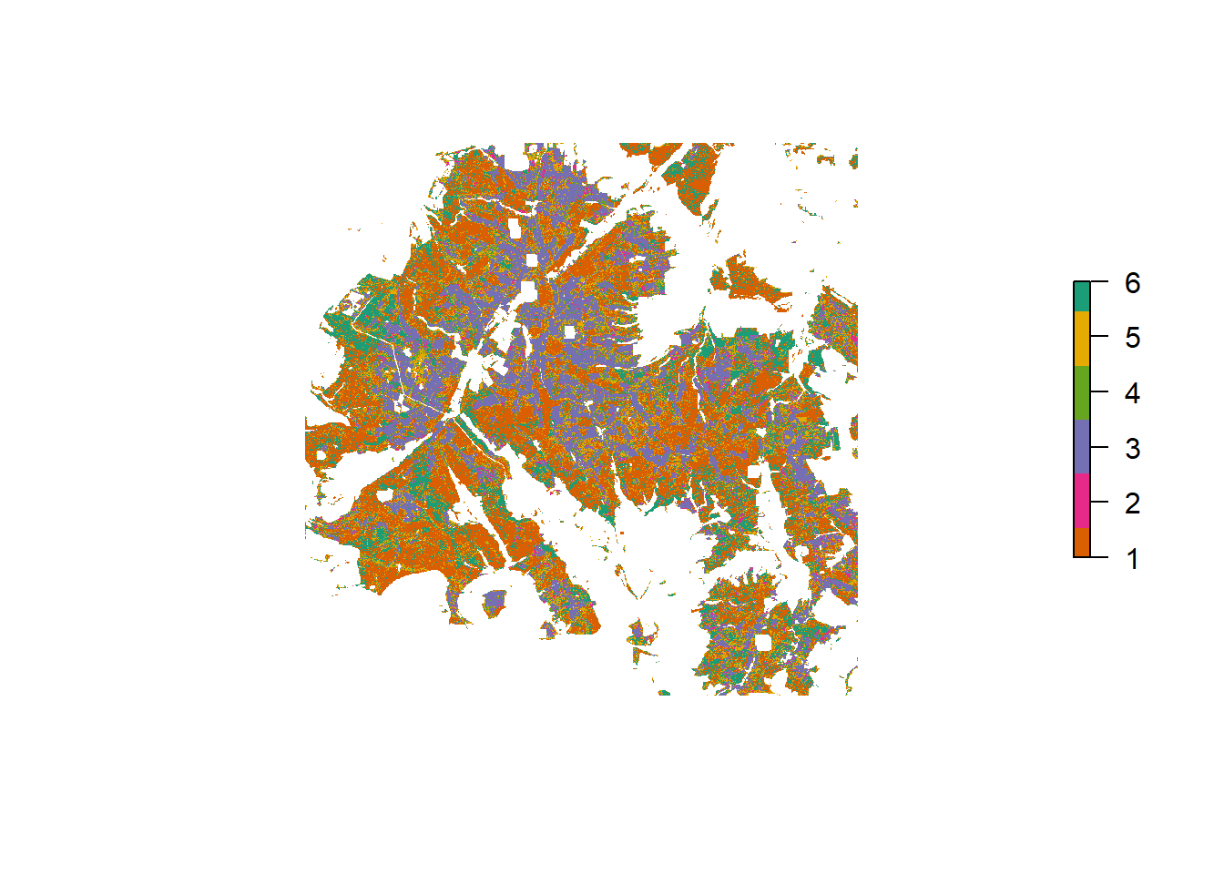
Tree species classification result for Solling
Harz
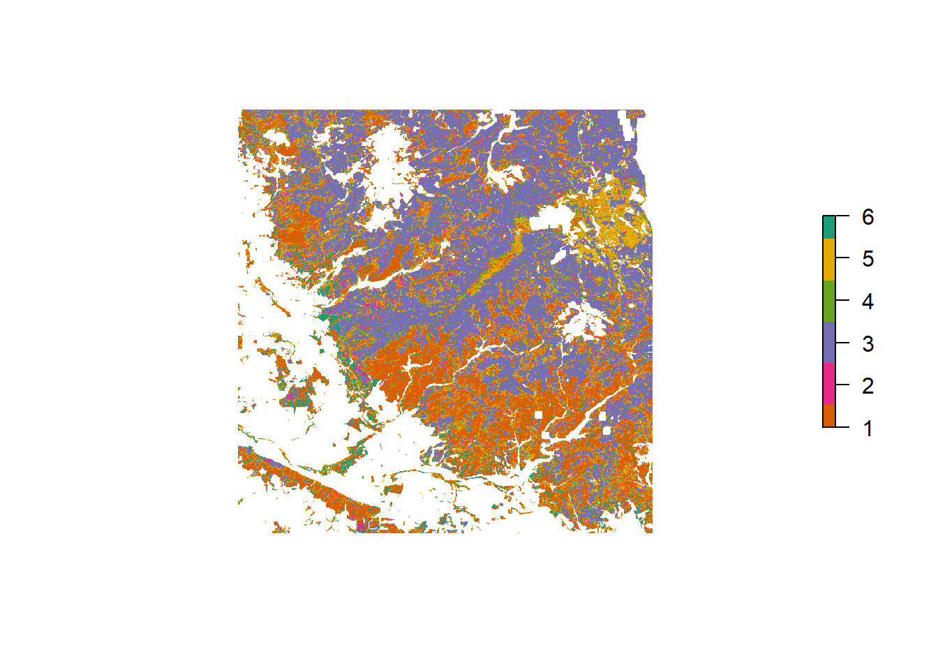
Tree species classification result for Harz
Heide
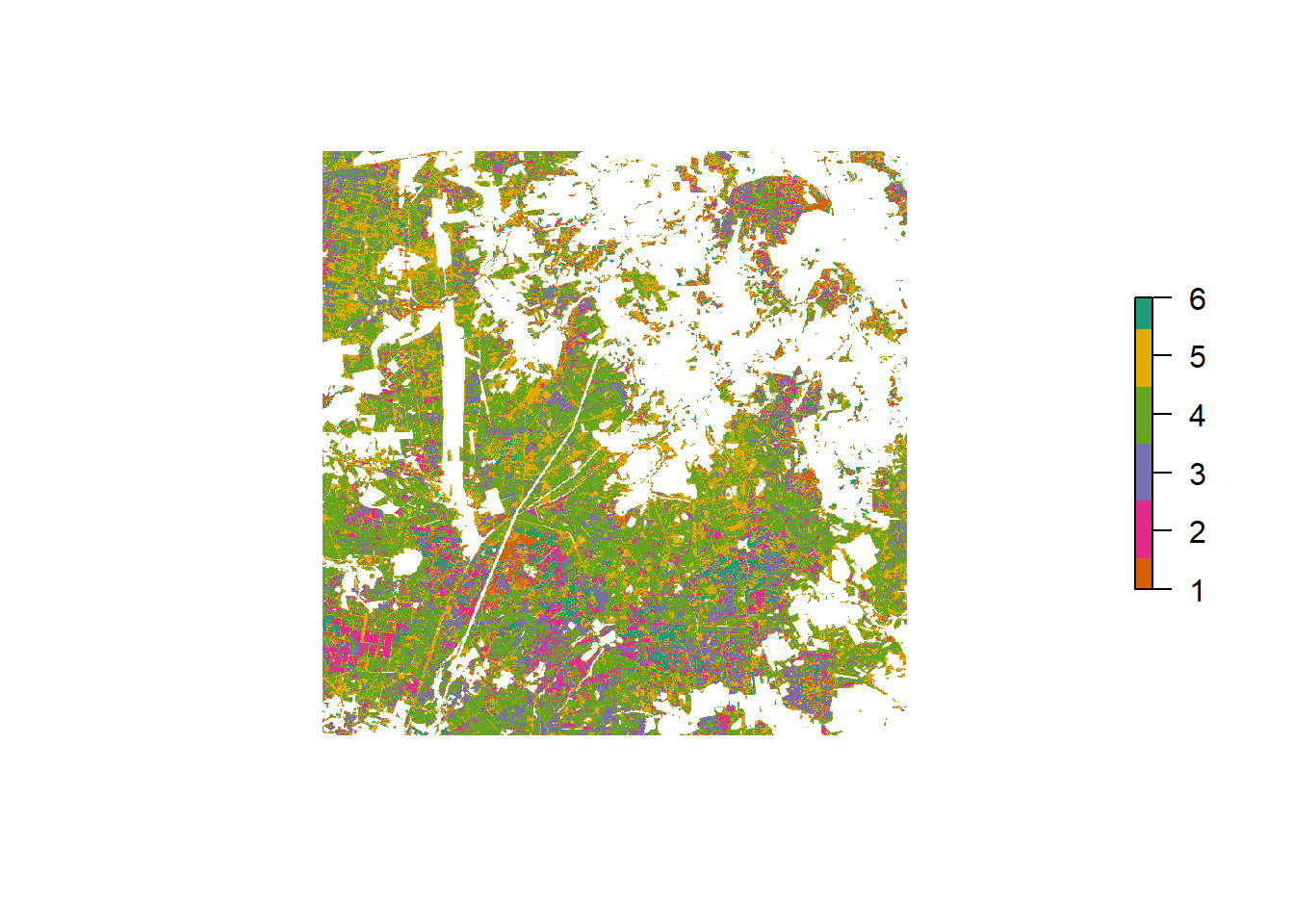
Tree species classification result for Heide
Probability
The Random Forest algorithm simply counts the fraction of trees in a forest that vote for a certain class to generate the predicted class. This class probability can be generated separately and provides insights in classification certainty.
Overview
Pixelwise classification probability (and average by latitude and longitiude) for the entire study region
Study sites
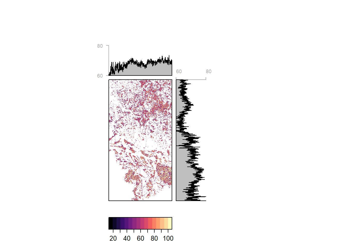
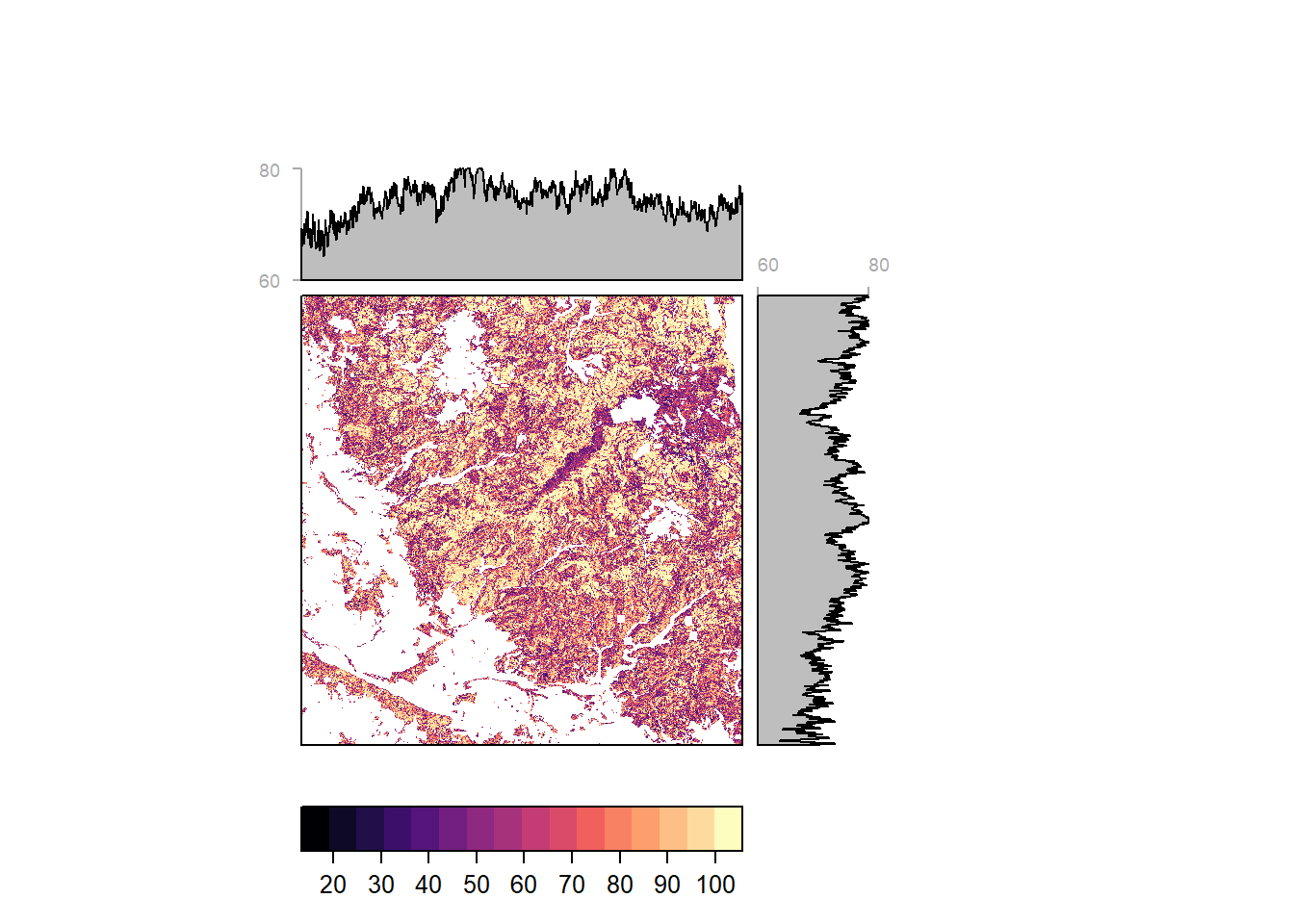
Solling
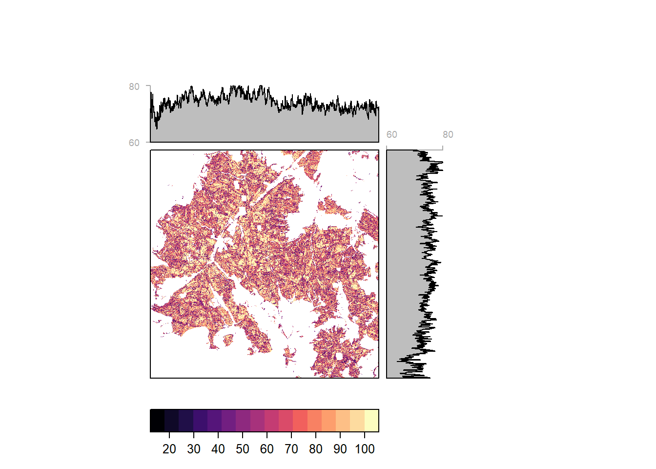
Pixelwise classification probability (and average by latitude and longitiude) for Solling
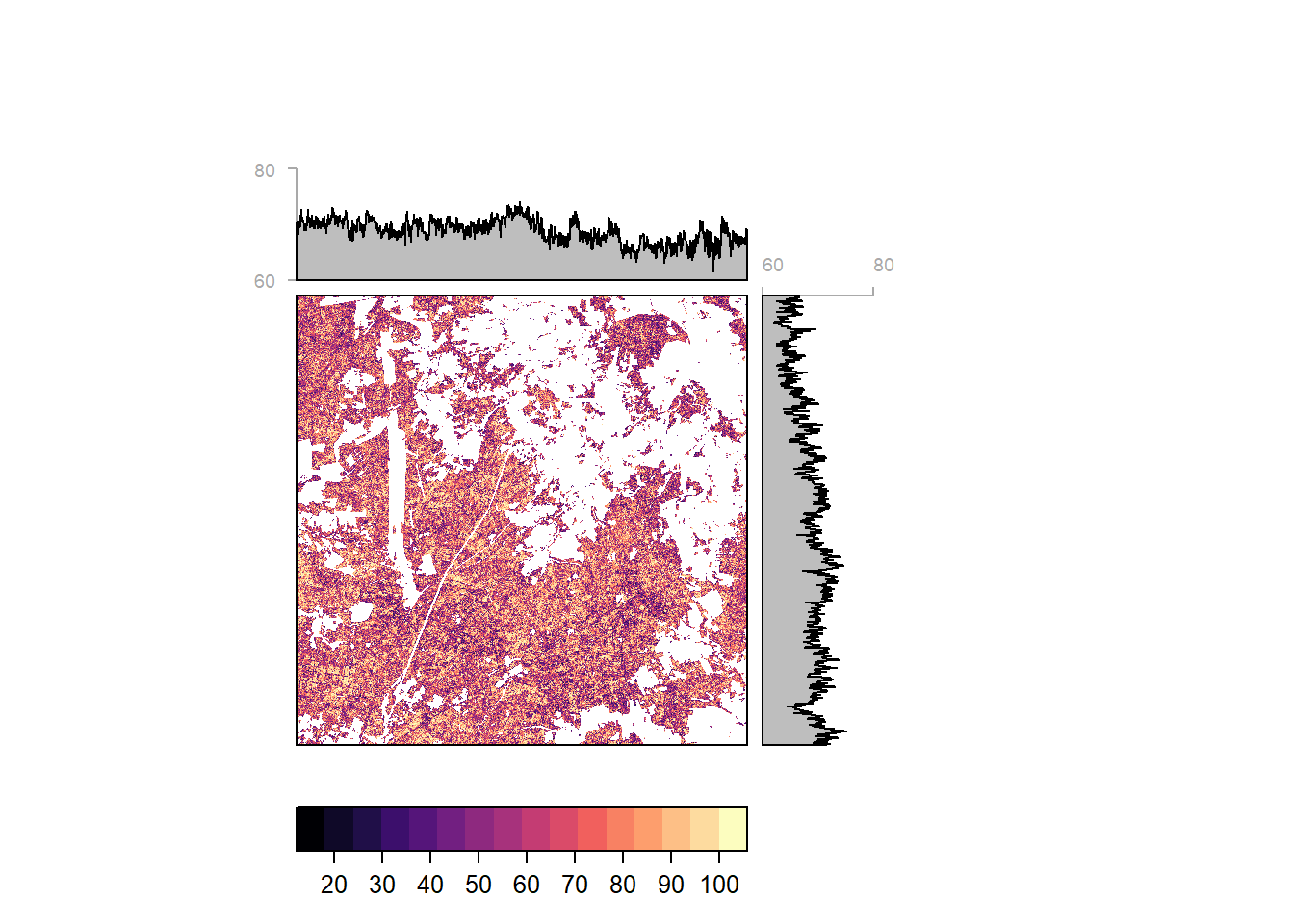
Harz
Pixelwise classification probability (and average by latitude and longitiude) for Harz
Heide
Pixelwise classification probability (and average by latitude and longitiude) for Heide
Reference Probability
Classification probabilities were extracted for each pixel inside reference polygons. The extracted values grant insight in classification certainty by tree species and reference site.
Classification probability by site and tree species for reference data locations
Reference Accuracy
Class predictions for all reference pixels were extracted from the model prediction raster. These predictions were thought to be compared with the reference data label to produce an error matrix. The accuracy was expected to be biased since we used part of the reference data for training the model. But instead, all reference data was classified correctly. This might suggest that the model is overfitted to the reference data, performing very well on the reference data but weaker outside.
Error Matrix| Eiche | Buche | Fichte | Douglasie | Kiefer | Laerche | |
|---|---|---|---|---|---|---|
| Eiche | 6082 | 0 | 0 | 0 | 0 | 0 |
| Buche | 0 | 8025 | 0 | 0 | 0 | 0 |
| Fichte | 0 | 0 | 9495 | 0 | 0 | 0 |
| Douglasie | 0 | 0 | 0 | 1760 | 0 | 0 |
| Kiefer | 0 | 0 | 0 | 0 | 1896 | 0 |
| Laerche | 0 | 0 | 0 | 0 | 0 | 3232 |
R version 4.0.2 (2020-06-22)
Platform: x86_64-w64-mingw32/x64 (64-bit)
Running under: Windows 10 x64 (build 18362)

Matrix products: default

locale:
[1] LC_COLLATE=German_Germany.1252  LC_CTYPE=German_Germany.1252
[3] LC_MONETARY=German_Germany.1252 LC_NUMERIC=C
[5] LC_TIME=German_Germany.1252

attached base packages:
[1] stats     graphics  grDevices utils     datasets  methods   base

other attached packages:
 [1] rasterVis_0.48      latticeExtra_0.6-29 kableExtra_1.1.0
 [4] RColorBrewer_1.1-2  caret_6.0-86        lattice_0.20-41
 [7] plotly_4.9.2.1      forcats_0.5.0       stringr_1.4.0
[10] dplyr_1.0.0         purrr_0.3.4         readr_1.3.1
[13] tidyr_1.1.0         tibble_3.0.3        ggplot2_3.3.2
[16] tidyverse_1.3.0     formattable_0.2.0.1 raster_3.3-13
[19] leaflet_2.0.3       rgdal_1.5-12        sp_1.4-2

loaded via a namespace (and not attached):
 [1] colorspace_1.4-1        ellipsis_0.3.1          class_7.3-17
 [4] rprojroot_1.3-2         fs_1.4.2                rstudioapi_0.11
 [7] hexbin_1.28.1           farver_2.0.3            prodlim_2019.11.13
[10] fansi_0.4.1             lubridate_1.7.9         xml2_1.3.2
[13] codetools_0.2-16        splines_4.0.2           knitr_1.29
[16] jsonlite_1.7.0          workflowr_1.6.2         pROC_1.16.2
[19] broom_0.7.0             dbplyr_1.4.4            png_0.1-7
[22] compiler_4.0.2          httr_1.4.2              backports_1.1.7
[25] assertthat_0.2.1        Matrix_1.2-18           lazyeval_0.2.2
[28] cli_2.0.2               later_1.1.0.1           leaflet.providers_1.9.0
[31] htmltools_0.5.0         tools_4.0.2             gtable_0.3.0
[34] glue_1.4.1              reshape2_1.4.4          Rcpp_1.0.5
[37] cellranger_1.1.0        vctrs_0.3.2             nlme_3.1-148
[40] iterators_1.0.12        crosstalk_1.1.0.1       timeDate_3043.102
[43] gower_0.2.2             xfun_0.15               rvest_0.3.6
[46] lifecycle_0.2.0         zoo_1.8-8               MASS_7.3-51.6
[49] scales_1.1.1            ipred_0.9-9             hms_0.5.3
[52] promises_1.1.1          parallel_4.0.2          yaml_2.2.1
[55] rpart_4.1-15            stringi_1.4.6           highr_0.8
[58] foreach_1.5.0           e1071_1.7-3             lava_1.6.7
[61] rlang_0.4.7             pkgconfig_2.0.3         evaluate_0.14
[64] recipes_0.1.13          htmlwidgets_1.5.1       tidyselect_1.1.0
[67] plyr_1.8.6              magrittr_1.5            R6_2.4.1
[70] generics_0.0.2          DBI_1.1.0               pillar_1.4.6
[73] haven_2.3.1             whisker_0.4             withr_2.2.0
[76] survival_3.2-3          nnet_7.3-14             modelr_0.1.8
[79] crayon_1.3.4            rmarkdown_2.3           jpeg_0.1-8.1
[82] grid_4.0.2              readxl_1.3.1            data.table_1.12.8
[85] blob_1.2.1              git2r_0.27.1            ModelMetrics_1.2.2.2
[88] reprex_0.3.0            digest_0.6.25           webshot_0.5.2
[91] httpuv_1.5.4            stats4_4.0.2            munsell_0.5.0
[94] viridisLite_0.3.0