Variance Regularization: Part Two
Jason Willwerscheid
3/11/2020
Last updated: 2020-03-12
Checks: 6 0
Knit directory: scFLASH/
This reproducible R Markdown analysis was created with workflowr (version 1.2.0). The Report tab describes the reproducibility checks that were applied when the results were created. The Past versions tab lists the development history.
Great! Since the R Markdown file has been committed to the Git repository, you know the exact version of the code that produced these results.
Great job! The global environment was empty. Objects defined in the global environment can affect the analysis in your R Markdown file in unknown ways. For reproduciblity it’s best to always run the code in an empty environment.
The command set.seed(20181103) was run prior to running the code in the R Markdown file. Setting a seed ensures that any results that rely on randomness, e.g. subsampling or permutations, are reproducible.
Great job! Recording the operating system, R version, and package versions is critical for reproducibility.
Nice! There were no cached chunks for this analysis, so you can be confident that you successfully produced the results during this run.
Great! You are using Git for version control. Tracking code development and connecting the code version to the results is critical for reproducibility. The version displayed above was the version of the Git repository at the time these results were generated.
Note that you need to be careful to ensure that all relevant files for the analysis have been committed to Git prior to generating the results (you can use wflow_publish or wflow_git_commit). workflowr only checks the R Markdown file, but you know if there are other scripts or data files that it depends on. Below is the status of the Git repository when the results were generated:
Ignored files:
    Ignored:    .DS_Store
    Ignored:    .Rhistory
    Ignored:    .Rproj.user/
    Ignored:    code/initialization/
    Ignored:    data-raw/10x_assigned_cell_types.R
    Ignored:    data/.DS_Store
    Ignored:    data/10x/
    Ignored:    data/Ensembl2Reactome.txt
    Ignored:    data/droplet.rds
    Ignored:    data/mus_pathways.rds
    Ignored:    output/backfit/
    Ignored:    output/final_montoro/
    Ignored:    output/lowrank/
    Ignored:    output/prior_type/
    Ignored:    output/pseudocount/
    Ignored:    output/pseudocount_redux/
    Ignored:    output/size_factors/
    Ignored:    output/var_type/

Untracked files:
    Untracked:  analysis/NBapprox.Rmd
    Untracked:  analysis/trachea4.Rmd
    Untracked:  code/alt_montoro/
    Untracked:  code/missing_data.R
    Untracked:  code/pulseseq/
    Untracked:  code/trachea4.R
    Untracked:  code/var_reg/
    Untracked:  fl_tmp.rds
    Untracked:  output/alt_montoro/
    Untracked:  output/pulseseq_fit.rds
    Untracked:  output/var_reg/

Unstaged changes:
    Modified:   code/utils.R
    Modified:   data-raw/pbmc.R
Note that any generated files, e.g. HTML, png, CSS, etc., are not included in this status report because it is ok for generated content to have uncommitted changes.
These are the previous versions of the R Markdown and HTML files. If you’ve configured a remote Git repository (see ?wflow_git_remote), click on the hyperlinks in the table below to view them.
| File | Version | Author | Date | Message |
|---|---|---|---|---|
| Rmd | f8991ba | Jason Willwerscheid | 2020-03-12 | wflow_publish(“./analysis/var_reg_pbmc2.Rmd”) |
Introduction
In a previous analysis, I put a prior on the residual variance parameters to prevent them from going to zero during the backfit (in the past, I had just been thresholding them). I fixed the prior rather than estimating it using empirical Bayes: as it turns out, the latter is simply not effective (I tried a range of prior families, including exponential and gamma priors).
Here, I combine the two approaches. I reason about Poisson mixtures to set a minimum threshold and then, after thresholding, I use empirical Bayes to shrink the variance estimates towards their mean.
As in the previous analysis, all fits add 20 factors greedily using point-normal priors and then backfit. Here, however, I don’t “pre-scale” cells (that is, I scale using library size normalization, but I don’t do any additional scaling based on cell-wise variance estimates). The code used to produce the fits can be viewed here.
Residual variance threshold
The “true” distribution of gene \(j\) can be modeled as \[ X_{ij} \sim \text{Poisson}(s_i \lambda_{ij}), \] where \(s_i\) is the size factor for cell \(i\) and \(\lambda_{ij}\) depends on, for example, cell type. The scaled entry \(Y_{ij} = X_{ij} / s_i\) then has variance \(\lambda_{ij} / s_i\). By the law of total variance, \(Y_j\) marginally has variance \[ \text{Var}(Y_j) \ge \mathbb{E}_i(\text{Var}(Y_{ij})) = \frac{1}{n} \sum_{i} \frac{\lambda_{ij}}{s_i} \approx \frac{1}{n} \sum_i Y_{ij} \]
Thus a reasonable lower bound for the residual variance estimates is \[ \min_j \frac{1}{n} \sum_i Y_{ij} \]
Prior family
I’ll use the family of gamma priors, since they have the advantage of being fast (unlike gamma and exponential mixtures) and yet flexible (as compared to one-parameter exponential priors).
Results: Variance Estimates
The regularization step doesn’t accomplish very much. Variance estimates are almost identical with and without it (the solid lines indicate the threshold):
suppressMessages(library(tidyverse))
suppressMessages(library(Matrix))

source("./code/utils.R")
pbmc <- readRDS("./data/10x/pbmc.rds")
pbmc <- preprocess.pbmc(pbmc)

res <- readRDS("./output/var_reg/varreg_fits2.rds")

var_df <- tibble(thresholded = res$unreg$fl$residuals.sd^2,
                 regularized = res$reg$fl$residuals.sd^2)

ggplot(var_df, aes(x = thresholded, y = regularized)) +
  geom_point(size = 1) +
  scale_x_log10() +
  scale_y_log10() +
  geom_abline(slope = 1, linetype = "dashed") +
  ggtitle("Variance Estimates") +
  geom_vline(xintercept = 1 / res$unreg$fl$flash.fit$given.tau) +
  geom_hline(yintercept = 1 / res$unreg$fl$flash.fit$given.tau)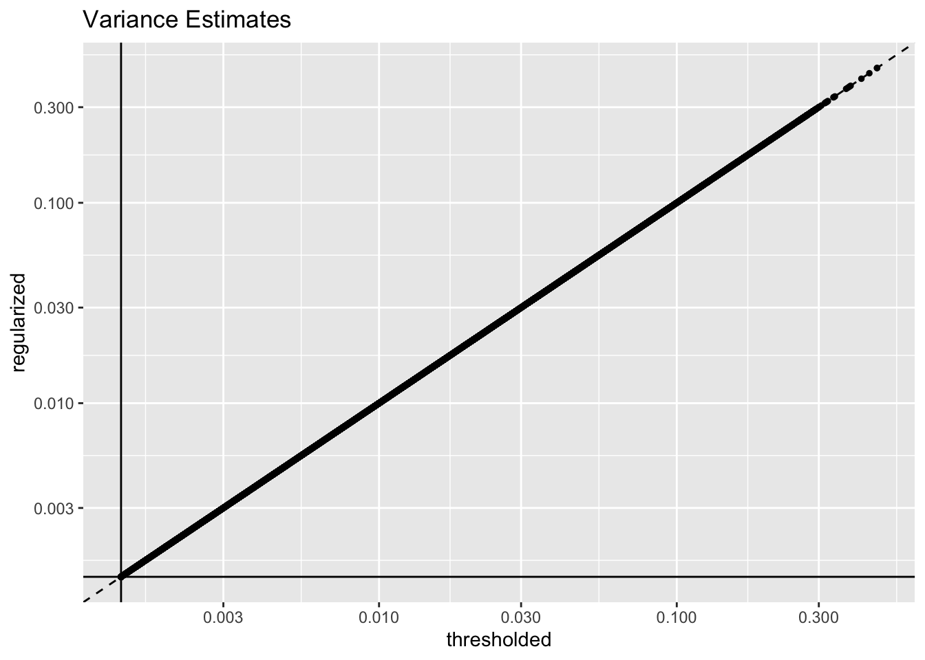
The regularized fit is slower and does worse with respect to both the ELBO (as expected) and the log likelihood of the implied discrete distribution (this is probably also to be expected).
res_df <- tibble(Fit = c("Thresholded", "Regularized"),
                 ELBO = sapply(res, function(x) x$fl$elbo),
                 Discrete.Llik = sapply(res, function(x) x$p.vals$llik),
                 Elapsed.Time = sapply(res, function(x) x$elapsed.time))
knitr::kable(res_df, digits = 0)| Fit | ELBO | Discrete.Llik | Elapsed.Time |
|---|---|---|---|
| Thresholded | 32318946 | -12497737 | 854 |
| Regularized | 32318983 | -12497566 | 1097 |
Results: Gene-wise thresholding
The argument I made above can in fact be applied gene by gene: that is, I can impose a gene-wise threshold rather than a single threshold for all genes. This argument rests on somewhat shakier ground, since I now need to use \(p\) plug-in estimators \[ \sum_i \hat{\lambda}_{ij} / s_i = \sum_i Y_{ij} \]
As it turns out, most estimates are very near their theoretical minimums. I’m not sure why this is the case. The code used to produce these fits can be viewed here.
res2 <- readRDS("./output/var_reg/varreg_fits3.rds")

var_df <- tibble(single.thresh = res$unreg$fl$residuals.sd^2,
                 genewise.thresh = res2$unreg$fl$residuals.sd^2,
                 theoretical.min = 1 / res2$unreg$fl$flash.fit$given.tau)

ggplot(var_df, aes(x = theoretical.min, y = genewise.thresh)) +
  geom_point(size = 1) +
  scale_x_log10() +
  scale_y_log10() +
  geom_abline(slope = 1, linetype = "dashed") +
  geom_vline(xintercept = 1 / res$unreg$fl$flash.fit$given.tau) +
  geom_hline(yintercept = 1 / res$unreg$fl$flash.fit$given.tau)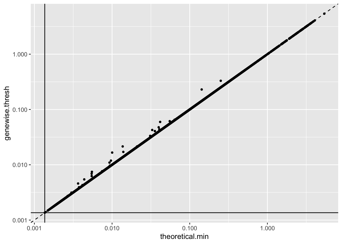
As a result, the gene-wise thresholding approach produces very different estimates. As I’ve previously argued, library-size normalization artificially reduces the variance of the most highly expressed genes (whence the parabola-like shape below):
ggplot(var_df, aes(x = single.thresh, y = genewise.thresh)) +
  geom_point(size = 1) +
  scale_x_log10() +
  scale_y_log10() +
  geom_abline(slope = 1, linetype = "dashed") +
  ggtitle("Variance Estimates") +
  geom_vline(xintercept = 1 / res$unreg$fl$flash.fit$given.tau) +
  geom_hline(yintercept = 1 / res$unreg$fl$flash.fit$given.tau)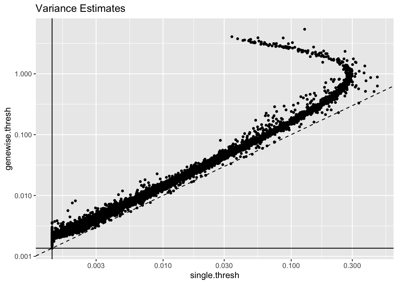
res_df <- res_df %>%
  bind_rows(tibble(Fit = c("Gene-wise Thresh", "Gene-wise Reg"),
                   ELBO = sapply(res2, function(x) x$fl$elbo),
                   Discrete.Llik = sapply(res2, function(x) x$p.vals$llik),
                   Elapsed.Time = sapply(res2, function(x) x$elapsed.time)))
knitr::kable(res_df, digits = 0)| Fit | ELBO | Discrete.Llik | Elapsed.Time |
|---|---|---|---|
| Thresholded | 32318946 | -12497737 | 854 |
| Regularized | 32318983 | -12497566 | 1097 |
| Gene-wise Thresh | 30172984 | -14036180 | 425 |
| Gene-wise Reg | 30172894 | -14036181 | 866 |
Results: Fixed variance estimates
Since most estimates are so close to their lower bounds, it might make sense to directly estimate the residual variances and then fix them rather than lower bounding them. I again use the law of total variance:
\[ \text{Var}(Y_j) = \mathbb{E}_i(\text{Var}(Y_{ij})) + \text{Var}_i(\mathbb{E}(Y_{ij})) = \frac{1}{n} \sum_{i} \frac{\lambda_{ij}}{s_i} + \text{Var}_i \frac{\lambda_{ij}}{s_i} \approx \frac{1}{n} \sum_i Y_{ij} + \text{Var}_i (Y_{ij}) \]
res3 <- readRDS("./output/var_reg/varreg_fits4.rds")

var_df <- tibble(fixed.estimates = res3$fl$residuals.sd^2,
                 lower.bd.estimates = res2$unreg$fl$residuals.sd^2)

ggplot(var_df, aes(x = lower.bd.estimates, y = fixed.estimates)) +
  geom_point(size = 1) +
  scale_x_log10() +
  scale_y_log10() +
  geom_abline(slope = 1, linetype = "dashed") +
  geom_vline(xintercept = 1 / res$unreg$fl$flash.fit$given.tau) +
  geom_hline(yintercept = 1 / res$unreg$fl$flash.fit$given.tau)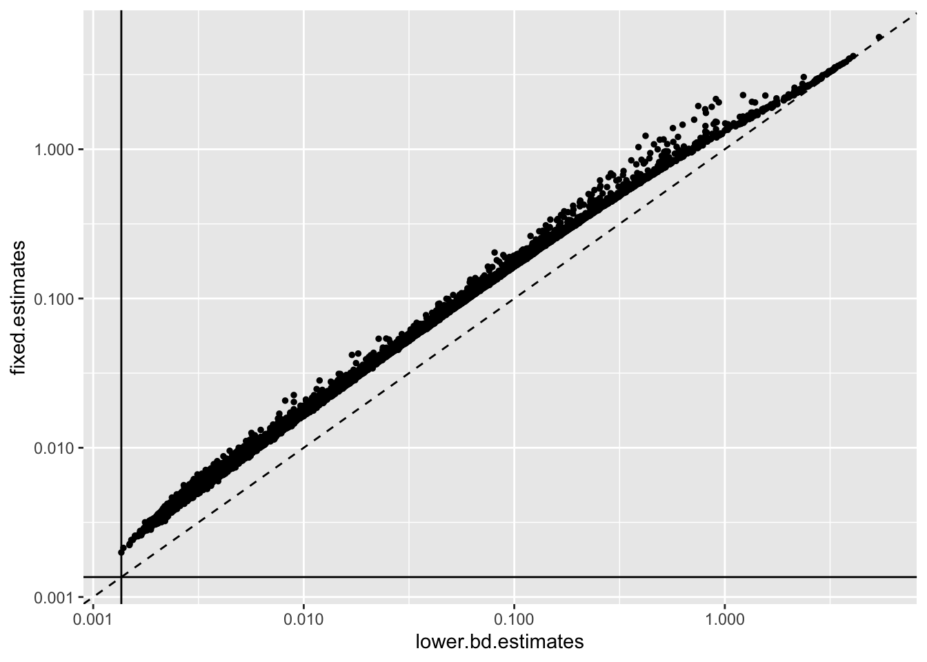
res_df <- res_df %>%
  bind_rows(tibble(Fit = "Fixed Estimates",
                   ELBO = res3$fl$elbo,
                   Discrete.Llik = res3$p.vals$llik,
                   Elapsed.Time = res3$elapsed.time))
knitr::kable(res_df, digits = 0)| Fit | ELBO | Discrete.Llik | Elapsed.Time |
|---|---|---|---|
| Thresholded | 32318946 | -12497737 | 854 |
| Regularized | 32318983 | -12497566 | 1097 |
| Gene-wise Thresh | 30172984 | -14036180 | 425 |
| Gene-wise Reg | 30172894 | -14036181 | 866 |
| Fixed Estimates | 24331805 | -15065854 | 162 |
Results: Factor comparisons
The more restrictive methods end up producing cleaner sets of factors: when fixed estimates are used, flash even terminates early, stopping after 9 factors have been added. The question, then, is whether the less restrictive methods yield additional information that’s biologically useful: do single threshold factors 5, 7, and 10, for example, better describe the CD4+/CD45RO+ axis than gene-wise threshold factor 6? or is factor 3 enough to describe this axis, as the fixed estimates results suggest? are three factors (6, 13, and 20) really needed to describe the rare CD34+ cell type?
plot.factors(res$unreg, pbmc$cell.type, kset = order(res$unreg$fl$pve, decreasing = TRUE),
             title = "Single threshold")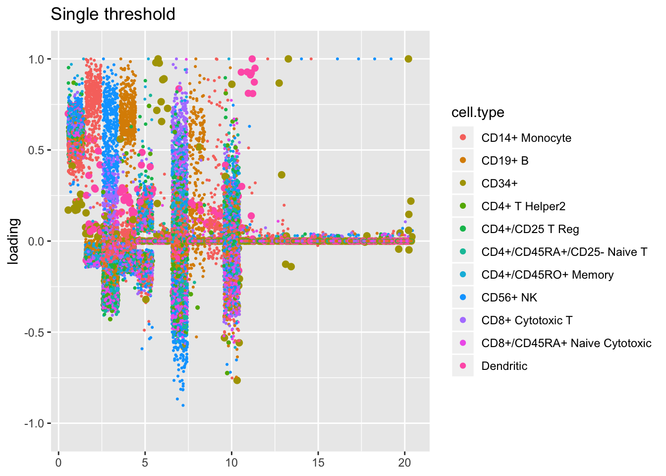
plot.factors(res2$unreg, pbmc$cell.type, kset = order(res2$unreg$fl$pve, decreasing = TRUE),
             title = "Gene-wise threshold")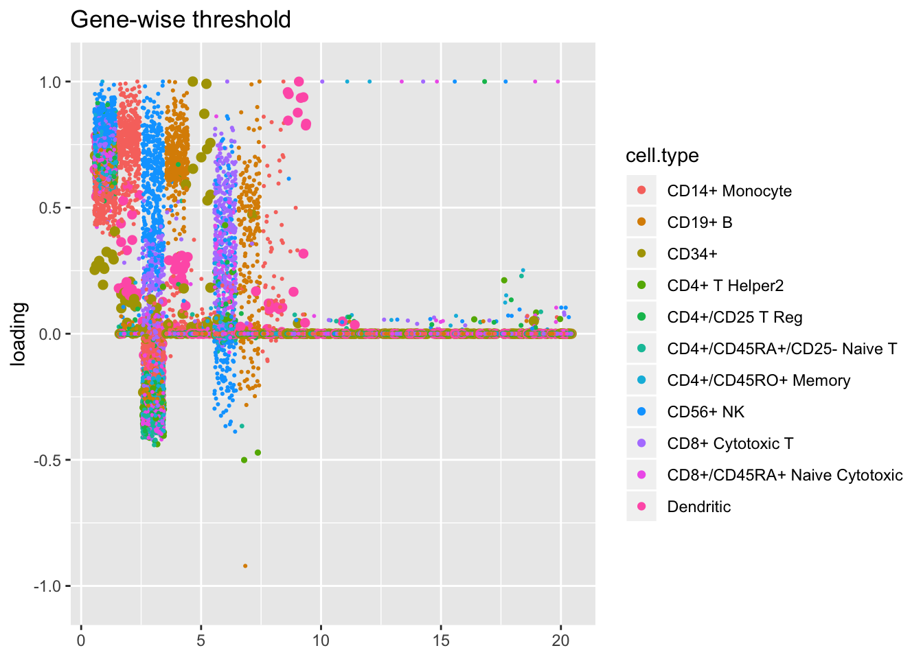
plot.factors(res3, pbmc$cell.type, kset = order(res3$fl$pve, decreasing = TRUE),
             title = "Fixed estimates")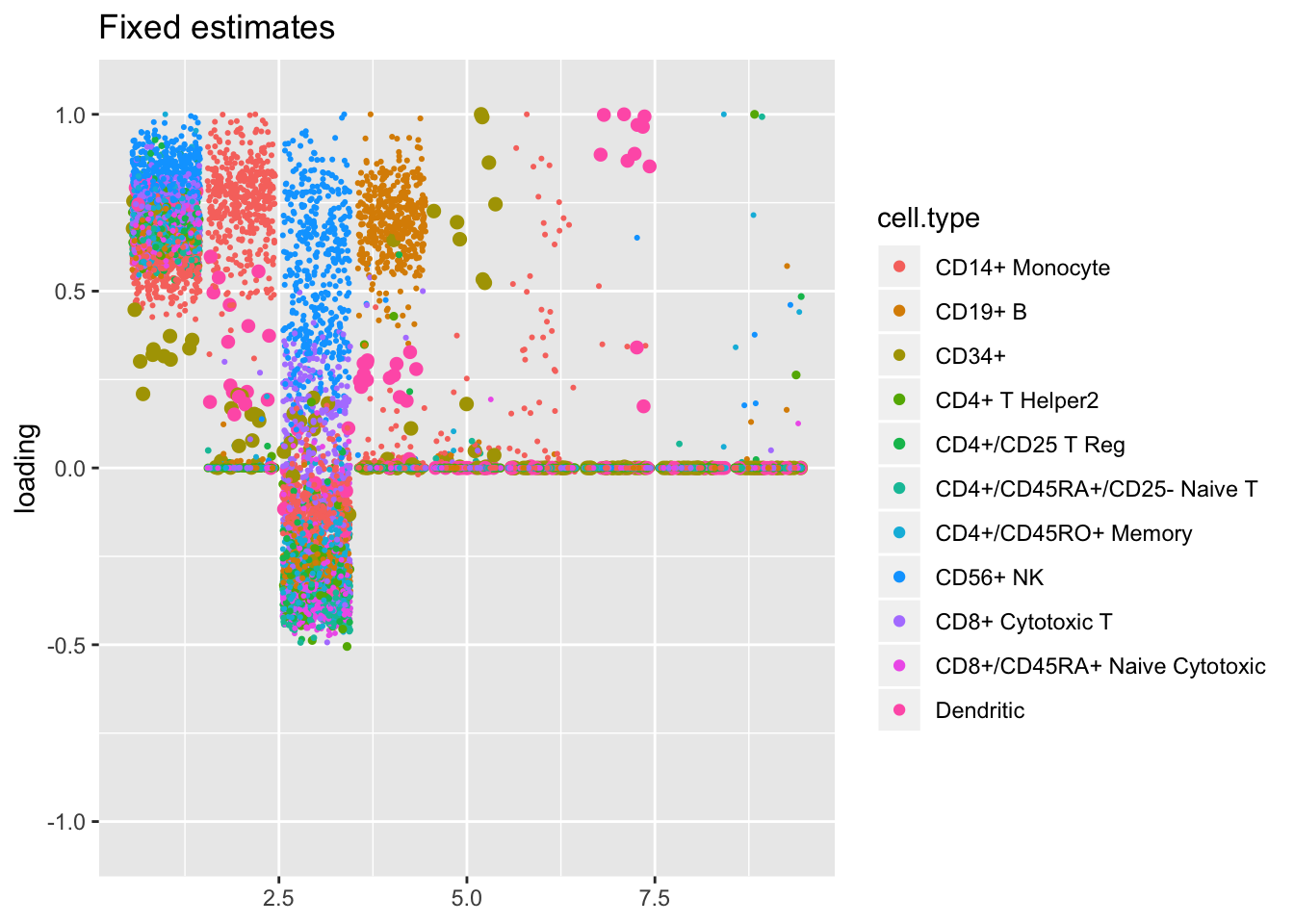
Results: PVE
pve_df <- tibble(method = "single.thresh",
                 pve = sort(res$unreg$fl$pve, decreasing = TRUE),
                 k = 1:length(res$unreg$fl$pve)) %>%
  bind_rows(tibble(method = "genewise.thresh",
                 pve = sort(res2$unreg$fl$pve, decreasing = TRUE),
                 k = 1:length(res2$unreg$fl$pve))) %>%
  bind_rows(tibble(method = "fixed.estimates",
                 pve = sort(res3$fl$pve, decreasing = TRUE),
                 k = 1:length(res3$fl$pve)))

ggplot(pve_df, aes(x = k, y = pve, col = method)) +
  geom_point() +
  geom_line() +
  scale_y_log10()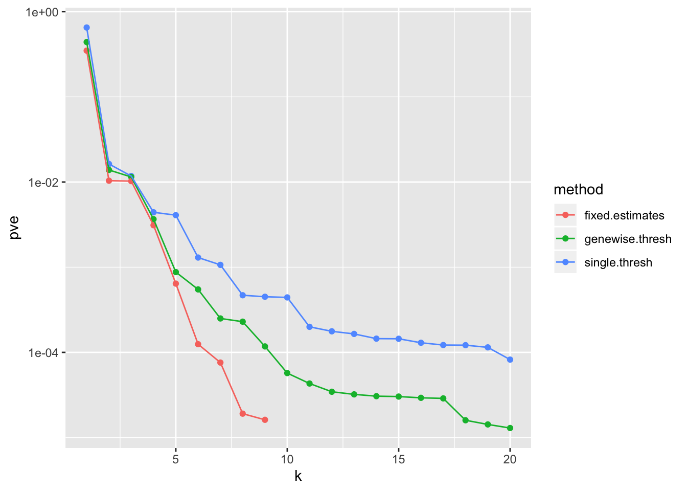
sessionInfo()R version 3.5.3 (2019-03-11)
Platform: x86_64-apple-darwin15.6.0 (64-bit)
Running under: macOS Mojave 10.14.6
Matrix products: default
BLAS: /Library/Frameworks/R.framework/Versions/3.5/Resources/lib/libRblas.0.dylib
LAPACK: /Library/Frameworks/R.framework/Versions/3.5/Resources/lib/libRlapack.dylib
locale:
[1] en_US.UTF-8/en_US.UTF-8/en_US.UTF-8/C/en_US.UTF-8/en_US.UTF-8
attached base packages:
[1] stats graphics grDevices utils datasets methods base
other attached packages:
[1] flashier_0.2.4 Matrix_1.2-15 forcats_0.4.0 stringr_1.4.0
[5] dplyr_0.8.0.1 purrr_0.3.2 readr_1.3.1 tidyr_0.8.3
[9] tibble_2.1.1 ggplot2_3.2.0 tidyverse_1.2.1
loaded via a namespace (and not attached):
[1] Rcpp_1.0.1 lubridate_1.7.4 lattice_0.20-38
[4] assertthat_0.2.1 rprojroot_1.3-2 digest_0.6.18
[7] foreach_1.4.4 truncnorm_1.0-8 R6_2.4.0
[10] cellranger_1.1.0 plyr_1.8.4 backports_1.1.3
[13] evaluate_0.13 httr_1.4.0 highr_0.8
[16] pillar_1.3.1 rlang_0.4.2 lazyeval_0.2.2
[19] pscl_1.5.2 readxl_1.3.1 rstudioapi_0.10
[22] ebnm_0.1-24 irlba_2.3.3 whisker_0.3-2
[25] rmarkdown_1.12 labeling_0.3 munsell_0.5.0
[28] mixsqp_0.3-17 broom_0.5.1 compiler_3.5.3
[31] modelr_0.1.5 xfun_0.6 pkgconfig_2.0.2
[34] SQUAREM_2017.10-1 htmltools_0.3.6 tidyselect_0.2.5
[37] workflowr_1.2.0 codetools_0.2-16 crayon_1.3.4
[40] withr_2.1.2 MASS_7.3-51.1 grid_3.5.3
[43] nlme_3.1-137 jsonlite_1.6 gtable_0.3.0
[46] git2r_0.25.2 magrittr_1.5 scales_1.0.0
[49] cli_1.1.0 stringi_1.4.3 reshape2_1.4.3
[52] fs_1.2.7 doParallel_1.0.14 xml2_1.2.0
[55] generics_0.0.2 iterators_1.0.10 tools_3.5.3
[58] glue_1.3.1 hms_0.4.2 parallel_3.5.3
[61] yaml_2.2.0 colorspace_1.4-1 ashr_2.2-38
[64] rvest_0.3.4 knitr_1.22 haven_2.1.1