Empirical inputs for simulations - IITA
2021-July-01
Last updated: 2021-07-14
Checks: 7 0
Knit directory: implementGMSinCassava/
This reproducible R Markdown analysis was created with workflowr (version 1.6.2). The Checks tab describes the reproducibility checks that were applied when the results were created. The Past versions tab lists the development history.
Great! Since the R Markdown file has been committed to the Git repository, you know the exact version of the code that produced these results.
Great job! The global environment was empty. Objects defined in the global environment can affect the analysis in your R Markdown file in unknown ways. For reproduciblity it’s best to always run the code in an empty environment.
The command set.seed(20210504) was run prior to running the code in the R Markdown file. Setting a seed ensures that any results that rely on randomness, e.g. subsampling or permutations, are reproducible.
Great job! Recording the operating system, R version, and package versions is critical for reproducibility.
Nice! There were no cached chunks for this analysis, so you can be confident that you successfully produced the results during this run.
Great job! Using relative paths to the files within your workflowr project makes it easier to run your code on other machines.
Great! You are using Git for version control. Tracking code development and connecting the code version to the results is critical for reproducibility.
The results in this page were generated with repository version 2953ee6. See the Past versions tab to see a history of the changes made to the R Markdown and HTML files.
Note that you need to be careful to ensure that all relevant files for the analysis have been committed to Git prior to generating the results (you can use wflow_publish or wflow_git_commit). workflowr only checks the R Markdown file, but you know if there are other scripts or data files that it depends on. Below is the status of the Git repository when the results were generated:
Ignored files:
    Ignored:    .DS_Store
    Ignored:    .Rhistory
    Ignored:    .Rproj.user/
    Ignored:    analysis/accuracies.png
    Ignored:    analysis/fig2.png
    Ignored:    analysis/fig3.png
    Ignored:    analysis/fig4.png
    Ignored:    code/.DS_Store
    Ignored:    data/.DS_Store

Untracked files:
    Untracked:  accuracies.png
    Untracked:  analysis/docs/
    Untracked:  analysis/speedUpPredCrossVar.Rmd
    Untracked:  code/AlphaAssign-Python/
    Untracked:  code/calcGameticLD.cpp
    Untracked:  code/col_sums.cpp
    Untracked:  code/convertDart2vcf.R
    Untracked:  code/helloworld.cpp
    Untracked:  code/imputationFunctions.R
    Untracked:  code/matmult.cpp
    Untracked:  code/misc.cpp
    Untracked:  code/test.cpp
    Untracked:  data/CassavaGeneticMap/
    Untracked:  data/DatabaseDownload_2021May04/
    Untracked:  data/GBSdataMasterList_31818.csv
    Untracked:  data/IITA_GBStoPhenoMaster_33018.csv
    Untracked:  data/NRCRI_GBStoPhenoMaster_40318.csv
    Untracked:  data/PedigreeGeneticGainCycleTime_aafolabi_01122020.xls
    Untracked:  data/blups_forCrossVal.rds
    Untracked:  data/chr1_RefPanelAndGSprogeny_ReadyForGP_72719.fam
    Untracked:  data/dosages_IITA_filtered_2021May13.rds
    Untracked:  data/genmap_2021May13.rds
    Untracked:  data/haps_IITA_filtered_2021May13.rds
    Untracked:  data/recombFreqMat_1minus2c_2021May13.rds
    Untracked:  fig2.png
    Untracked:  fig3.png
    Untracked:  figure/
    Untracked:  output/IITA_CleanedTrialData_2021May10.rds
    Untracked:  output/IITA_ExptDesignsDetected_2021May10.rds
    Untracked:  output/IITA_blupsForModelTraining_twostage_asreml_2021May10.rds
    Untracked:  output/IITA_trials_NOT_identifiable.csv
    Untracked:  output/crossValPredsA.rds
    Untracked:  output/crossValPredsAD.rds
    Untracked:  output/cvAD_5rep5fold_markerEffects.rds
    Untracked:  output/cvAD_5rep5fold_meanPredAccuracy.rds
    Untracked:  output/cvAD_5rep5fold_parentfolds.rds
    Untracked:  output/cvAD_5rep5fold_predMeans.rds
    Untracked:  output/cvAD_5rep5fold_predVars.rds
    Untracked:  output/cvAD_5rep5fold_varPredAccuracy.rds
    Untracked:  output/cvDirDom_5rep5fold_markerEffects.rds
    Untracked:  output/cvDirDom_5rep5fold_meanPredAccuracy.rds
    Untracked:  output/cvDirDom_5rep5fold_parentfolds.rds
    Untracked:  output/cvDirDom_5rep5fold_predMeans.rds
    Untracked:  output/cvDirDom_5rep5fold_predVars.rds
    Untracked:  output/cvDirDom_5rep5fold_varPredAccuracy.rds
    Untracked:  output/cvMeanPredAccuracyA.rds
    Untracked:  output/cvMeanPredAccuracyAD.rds
    Untracked:  output/cvPredMeansA.rds
    Untracked:  output/cvPredMeansAD.rds
    Untracked:  output/cvVarPredAccuracyA.rds
    Untracked:  output/cvVarPredAccuracyAD.rds
    Untracked:  output/genomicPredictions_ModelAD.rds
    Untracked:  output/genomicPredictions_ModelDirDom.rds
    Untracked:  output/kinship_A_IITA_2021May13.rds
    Untracked:  output/kinship_D_IITA_2021May13.rds
    Untracked:  output/markEffsTest.rds
    Untracked:  output/markerEffects.rds
    Untracked:  output/markerEffectsA.rds
    Untracked:  output/markerEffectsAD.rds
    Untracked:  output/maxNOHAV_byStudy.csv
    Untracked:  output/obsCrossMeansAndVars.rds
    Untracked:  output/parentfolds.rds
    Untracked:  output/ped2check_genome.rds
    Untracked:  output/ped2genos.txt
    Untracked:  output/pednames2keep.txt
    Untracked:  output/pednames_Prune100_25_pt25.log
    Untracked:  output/pednames_Prune100_25_pt25.nosex
    Untracked:  output/pednames_Prune100_25_pt25.prune.in
    Untracked:  output/pednames_Prune100_25_pt25.prune.out
    Untracked:  output/potential_dams.txt
    Untracked:  output/potential_sires.txt
    Untracked:  output/predVarTest.rds
    Untracked:  output/samples2keep_IITA_2021May13.txt
    Untracked:  output/samples2keep_IITA_MAFpt01_prune50_25_pt98.log
    Untracked:  output/samples2keep_IITA_MAFpt01_prune50_25_pt98.nosex
    Untracked:  output/samples2keep_IITA_MAFpt01_prune50_25_pt98.prune.in
    Untracked:  output/samples2keep_IITA_MAFpt01_prune50_25_pt98.prune.out
    Untracked:  output/verified_ped.txt
Note that any generated files, e.g. HTML, png, CSS, etc., are not included in this status report because it is ok for generated content to have uncommitted changes.
These are the previous versions of the repository in which changes were made to the R Markdown (analysis/inputsForSimulation.Rmd) and HTML (docs/inputsForSimulation.html) files. If you’ve configured a remote Git repository (see ?wflow_git_remote), click on the hyperlinks in the table below to view the files as they were in that past version.
| File | Version | Author | Date | Message |
|---|---|---|---|---|
| html | 3a1faa0 | wolfemd | 2021-07-14 | Build site. |
| Rmd | 134c8d3 | wolfemd | 2021-07-14 | Publish first pass at GS pipeline-integrated estimation of selection error for input into simulations downstream. |
# pull a singularity image and save in the file rocker.sif
# singularity pull ~/rocker2.sif docker://rocker/tidyverse;

# 1) start a screen shell
screen; # or screen -r if re-attaching...
# 2) start the singularity Linux shell inside that
singularity shell ~/rocker2.sif;
#singularity shell /workdir/$USER/rocker.sif;
# Project directory, so R will use as working dir.
cd /home/mw489/implementGMSinCassava/;
# 3) Start R
R
Concept
We want to simulate the advantages of different breeding pipelines (variety development pipelines; VDPs) based on proposed differences in plot-size (number of plants), number of reps, locations and overall trial-stage size.
Question: How do we empirically know what difference varying these parameters is associated with?
We can’t compute the selection index per se for each trial because of variation in the traits scored. Then again, neither can breeders.
We want:
- an objective approach to estimate the selection error for an SI on a trial-by-trail basis,
- ideally using existing GS pipeline / data,
- dealing with heterogeneity in traits-observed in given trial.
Proposed approach:
Generate a best estimate of “true” net merit using the SELECTION INDEX GEBV/GETGV from full genomic prediction, i.e. the entire available training population and all of the latest available data. The predictions made here are the most up-to-date.
- Alternative best estimate of “true” net merit: actual national performance trial data (e.g. from NCRPs in Nigeria?)
For each trial, and each trait scored:
Fit mixed-model
Extract trial-specific BLUPs
Compute the SELIND for the current trial using BLUPs for whatever component traits were scored (\(SI_{TrialBLUP}\)).
Regress \(SI_{GETGV}\) on the \(SI_{TrialBLUP}\)
- Extract the \(\sigma^2_e\) of the regression as the trial-specific estimate of the selection error
Finally, the relationship between SI error and plot-size can be plotted and a function for SI error given plot-size can be developed that can be plugged into simulations of any VDP of interest.
Selection Index GETGV: proxy for true net merit
- Generate a best estimate of “true” net merit using the SELECTION INDEX GETGV from full genomic prediction, i.e. the entire available training population and all of the latest available data. The predictions made here are the most up-to-date.
library(tidyverse); library(magrittr);
# GBLUPs
### Two models AD and DirDom
#gpreds_ad<-readRDS(file = here::here("output","genomicPredictions_ModelAD.rds"))
gpreds_dirdom<-readRDS(file = here::here("output","genomicPredictions_ModelDirDom.rds"))
si_getgvs<-gpreds_dirdom$gblups[[1]] %>%
#si_getgvs<-gpreds_ad$gblups[[1]] %>%
  filter(predOf=="GETGV") %>%
  select(GID,SELIND)

## IITA Germplasm Ages
ggcycletime<-readxl::read_xls(here::here("data","PedigreeGeneticGainCycleTime_aafolabi_01122020.xls")) %>%
  mutate(Year_Accession=as.numeric(Year_Accession))

# Need germplasmName field from raw trial data to match GEBV and cycle time
dbdata<-readRDS(here::here("output","IITA_ExptDesignsDetected_2021May10.rds"))
si_getgvs %<>%
  left_join(dbdata %>%
              distinct(germplasmName,GID)) %>%
  group_by(GID) %>%
  slice(1) %>%
  ungroup()
# table(ggcycletime$Accession %in% si_getgvs$germplasmName)
# FALSE  TRUE
#   193   614

si_getgvs %<>%
  left_join(.,ggcycletime %>%
              rename(germplasmName=Accession) %>%
              mutate(Year_Accession=as.numeric(Year_Accession))) %>%
  mutate(Year_Accession=case_when(grepl("2013_|TMS13",germplasmName)~2013,
                                  grepl("TMS14",germplasmName)~2014,
                                  grepl("TMS15",germplasmName)~2015,
                                  grepl("TMS18",germplasmName)~2018,
                                  !grepl("2013_|TMS13|TMS14|TMS15|TMS18",germplasmName)~Year_Accession))

# Declare the "eras" as PreGS\<2012 and GS\>=2013.
si_getgvs %<>%
  filter(Year_Accession>2012 | Year_Accession<2005)
si_getgvs %<>%
  mutate(GeneticGroup=ifelse(Year_Accession>=2013,"GS","PreGS"))

# SELECTION INDEX WEIGHTS
## from IYR+IK
## note that not ALL predicted traits are on index
SIwts<-c(logFYLD=20,
         HI=10,
         DM=15,
         MCMDS=-10,
         logRTNO=12,
         logDYLD=20,
         logTOPYLD=15,
         PLTHT=10)

# SELIND GETGVS (for input to estimateSelectionError func below)
getgvs<-si_getgvs %>%
  select(GID,SELIND);
# , fig.height=10, fig.width=12
si_getgvs %>%
select(GeneticGroup,GID,Year_Accession,SELIND) %>%
ggplot(.,aes(x=Year_Accession,y=SELIND,color=GeneticGroup)) +
geom_point(size=1.25) + geom_smooth(method=lm, se=TRUE, size=1.5) +
# facet_wrap(~Trait,scales='free_y', ncol=2) +
theme_bw() +
theme(axis.text = element_text(face = 'bold',angle = 0, size=14),
axis.title = element_text(face = 'bold',size=16),
strip.background.x = element_blank(),
strip.text = element_text(face='bold',size=18)) +
scale_color_viridis_d() +
labs(title = "Selection Index GETGV vs. Accession Age by 'era' [GS vs. PreGS]",
subtitle = "SI GETGV from modelType='DirDom'")
| Version | Author | Date |
|---|---|---|
| 3a1faa0 | wolfemd | 2021-07-14 |
si_gebvs<-gpreds_dirdom$gblups[[1]] %>%
  filter(predOf=="GEBV") %>%
  select(GID,SELIND) %>%
  mutate(GeneticGroup=case_when(grepl("2013_|TMS13",GID)~"C1",
                                  grepl("TMS14",GID)~"C2",
                                  grepl("TMS15",GID)~"C3",
                                  grepl("TMS18",GID)~"C4",
                                  !grepl("2013_|TMS13|TMS14|TMS15|TMS18",GID)~"PreGS"),
         GeneticGroup=factor(GeneticGroup,levels = c("PreGS","C1","C2","C3","C4")))
si_gebvs %>%
  group_by(GeneticGroup) %>%
  summarize(meanGEBV=mean(SELIND),
            stdErr=sd(SELIND)/sqrt(n()),
            upperSE=meanGEBV+stdErr,
            lowerSE=meanGEBV-stdErr) %>%
  ggplot(.,aes(x=GeneticGroup,y=meanGEBV,fill=GeneticGroup)) +
  geom_bar(stat = 'identity', color='gray60', size=1.25) +
  geom_linerange(aes(ymax=upperSE,
                     ymin=lowerSE), color='gray60', size=1.25) +
  #facet_wrap(~Trait,scales='free_y', ncol=1) +
  theme_bw() +
  geom_hline(yintercept = 0, size=1.15, color='black') +
  theme(axis.text.x = element_text(face = 'bold',angle = 0, size=12),
        axis.title.y = element_text(face = 'bold',size=14),
        legend.position = 'none',
        strip.background.x = element_blank(),
        strip.text = element_text(face='bold',size=14)) +
  scale_fill_viridis_d() +
  labs(x=NULL,y="Mean GEBVs")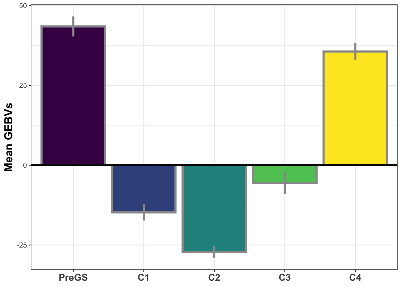
| Version | Author | Date |
|---|---|---|
| 3a1faa0 | wolfemd | 2021-07-14 |
Estimate selection error for each trial
For each trial, and each trait scored:
Fit mixed-model
Extract trial-specific BLUPs
Compute the SELIND for the current trial using BLUPs for whatever component traits were scored (\(SI_{TrialBLUP}\)).
Regress \(SI_{GETGV}\) on the \(SI_{TrialBLUP}\)
- Extract the \(\sigma^2_e\) of the regression as the trial-specific estimate of the selection error
Available plot-level data
See here for details about the cleaned trial data most recently downloaded from IITA/Cassavabase and used below.
Quick summary of the number of unique plots, locations, years, etc. in the cleaned plot-basis data.
dbdata %>%
  summarise(Nplots=nrow(.),
            across(c(locationName,studyYear,studyName,TrialType,GID), ~length(unique(.)),.names = "N_{.col}")) %>%
  rmarkdown::paged_table()
dbdata %>%
count(TrialType,CompleteBlocks,IncompleteBlocks) %>%
spread(TrialType,n) %>%
rmarkdown::paged_table()Not much NCRP data, but there is some.
dbdata %>%
  filter(studyYear>=2013) %>%
  distinct(studyYear,locationName,studyName,TrialType,CompleteBlocks,IncompleteBlocks,MaxNOHAV) %>%
  filter(!is.na(MaxNOHAV)) %>% #count(TrialType)
  mutate(TrialType=factor(TrialType,levels=c("CrossingBlock","GeneticGain","CET","ExpCET","PYT","AYT","UYT","NCRP"))) %>%
  ggplot(.,aes(x=TrialType,y=MaxNOHAV,fill=TrialType)) +
  geom_boxplot(notch = T) +
  theme_bw() + theme(axis.text.x = element_text(angle=45,vjust=.5)) +
  labs(title = "Max number harvested as a proxy for planned plot size",
       subtitle="MaxNOHAV = The maximum number stands harvested per trial")
| Version | Author | Date |
|---|---|---|
| 3a1faa0 | wolfemd | 2021-07-14 |
Trial-by-trial mixed-models
Decided it makes sense to restrict consideration to >2012 to measure the selection error during the current “era” at IITA.
trials2keep<-dbdata %>%
  filter(studyYear>=2013) %>%
  distinct(studyYear,locationName,studyName,TrialType,CompleteBlocks,IncompleteBlocks,MaxNOHAV) %>%
  filter(!is.na(MaxNOHAV)) %$%
  unique(studyName)
# 633 trials, 94830 plots

trialdata<-dbdata %>%
  filter(studyYear>=2013,
         studyName %in% trials2keep) %>%
  nest(TrialData=-c(studyYear,locationName,studyName,TrialType,CompleteBlocks,IncompleteBlocks,MaxNOHAV))

trialdata %<>%
  mutate(propGenotyped=map_dbl(TrialData,
                              ~length(which(!is.na(unique(.$FullSampleName))))/length(unique(.$GID))))

trialdata %>% head
# A tibble: 6 x 9
studyYear locationName studyName TrialType MaxNOHAV CompleteBlocks
<int> <chr> <chr> <chr> <dbl> <lgl>
1 2013 Ikenne 13Ayt15HtcIK AYT 10 TRUE
2 2013 Ibadan 13Ayt16ICTIB AYT 10 TRUE
3 2013 Ikenne 13Ayt17HtcIK AYT 10 TRUE
4 2013 Ibadan 13ayt20pdIB AYT 10 TRUE
5 2013 Ibadan 13ayt20pdwhtrtIB AYT 10 TRUE
6 2013 Ibadan 13ayt20pdyrtIB AYT 10 TRUE
# … with 3 more variables: IncompleteBlocks <lgl>, TrialData <list>,
# propGenotyped <dbl># TrialData<-trialdata$TrialData[[1]]
# CompleteBlocks<-trialdata$CompleteBlocks[[1]]
# IncompleteBlocks<-trialdata$IncompleteBlocks[[1]]
#
# TrialData<-trialdata %>% filter(propGenotyped>0.75) %>% slice(4) %$% TrialData[[1]]
# CompleteBlocks<-trialdata %>% filter(propGenotyped>0.75) %>% slice(4) %$% CompleteBlocks[[1]]
# IncompleteBlocks<-trialdata %>% filter(propGenotyped>0.75) %>% slice(4) %$% IncompleteBlocks[[1]]
# ncores=4
# rm(TrialData,CompleteBlocks,IncompleteBlocks)Function to estimation selection error for each trial: estimateSelectionError().
estimateSelectionError<-possibly(function(TrialData,CompleteBlocks,IncompleteBlocks,
                                 SIwts,getgvs,...){

  # SET-UP THE DATA TRAIT-BY-TRIAL~~~~~~~~~~~~~~~~~~~~~
  blups<-TrialData %>%
    select(observationUnitDbId,GID,plotNumber,repInTrial,blockInRep,PropNOHAV,
           all_of(names(SIwts))) %>%
    pivot_longer(cols = c(all_of(names(SIwts))),
                 names_to = "Trait",
                 values_to = "TraitValue") %>%
    nest(TraitByTrialData=c(-Trait))

  # FIT MIXED-MODELS TRAIT-BY-TRIAL~~~~~~~~~~~~~~~~~~~~~~

  ## if model fails, by design, returns NULL for a given trait or trait-trial
  ## Output will simply be absent.
  fit_model<-possibly(function(Trait,TraitByTrialData,CompleteBlocks,IncompleteBlocks){
    # debug settings ~~~~~~~~~~
    # TraitByTrialData<-blups$TraitByTrialData[[1]]
    # Trait<-blups$Trait[[1]]
    # TraitByTrialData<-blups$TraitByTrialData[[8]]
    # Trait<-blups$Trait[[8]]
    # rm(TraitByTrialData,Trait)

    # Model formula based on trial design
    modelFormula<-paste0("TraitValue ~ (1|GID)")
    modelFormula<-ifelse(CompleteBlocks,
                         paste0(modelFormula,"+(1|repInTrial)"),modelFormula)
    modelFormula<-ifelse(IncompleteBlocks,
                         paste0(modelFormula,"+(1|blockInRep)"),modelFormula)
    modelFormula<-ifelse(Trait %in% c("logRTNO","logFYLD","logTOPYLD","logDYLD"),
                         paste0(modelFormula,"+PropNOHAV"),modelFormula)
    require(lme4); require(lme4)
    model_out<-lmer(as.formula(modelFormula),data=TraitByTrialData)
    propMiss<-length(which(is.na(TraitByTrialData$TraitValue))) / length(TraitByTrialData$TraitValue)

    if(is.na(model_out) | !exists("model_out")){
      out <-tibble(H2=NA,VarComps=list(NULL),BLUPs=list(NULL),Model=modelFormula,propMiss=propMiss)
    } else {
      varcomps<-as.data.frame(VarCorr(model_out))[,c("grp","vcov")] %>%
        spread(grp,vcov)
      Vg<-varcomps$GID
      H2<-Vg/(Vg+varcomps$Residual)
      BLUP<-ranef(model_out, condVar=TRUE)[["GID"]]
      PEV <- c(attr(BLUP, "postVar"))
      blup<-tibble(GID=rownames(BLUP),BLUP=BLUP$`(Intercept)`,PEV=PEV) %>%
        mutate(REL=1-(PEV/Vg),
               drgBLUP=BLUP/REL,
               WT=(1-H2)/((0.1 + (1-REL)/REL)*H2))
      out <- tibble(H2=H2,
                    VarComps=list(varcomps),
                    BLUPs=list(blup),
                    Model=modelFormula,
                    propMiss=propMiss) }
    return(out) },
    otherwise = NULL)

  blups %<>%
    mutate(modelOut=pmap(.,fit_model,
                         CompleteBlocks=CompleteBlocks,
                         IncompleteBlocks=IncompleteBlocks)) %>%
    select(-TraitByTrialData) %>%
    unnest(modelOut) %>%
    unnest(VarComps)

  # COMPUTE SELIND FROM BLUPs~~~~~~~~~~~~~~~~~~~~~~
  si_blups<-blups %>%
    select(Trait,BLUPs) %>%
    unnest(BLUPs) %>%
    select(GID,Trait,BLUP) %>%
    spread(Trait,BLUP) %>%
    select(GID,any_of(names(SIwts))) %>%
    column_to_rownames(var = "GID") %>%
    as.matrix
  si_blups<-si_blups%*%SIwts[colnames(si_blups)] %>%
    as.data.frame %>%
    rownames_to_column(var = "GID") %>%
    rename(SI_BLUP=V1) %>%
    left_join(getgvs)

  # Correlation between SELIND (SI GETGV) and the SI of BLUPs for current trial
  cor2si<-si_blups %$% cor(SI_BLUP,SELIND,use = 'complete.obs')

  # Regress SELIND on SI_BLUPs
  regSIonTrialBLUP<-lm(SELIND~SI_BLUP,data = si_blups)

  # TWO MEASURES OF SELECTION ERROR
  ## 1) regression r-squared [or 1 - r2_si actually]
  ## 2) mean squared error,
  ##### not sure if the scaling will make sense across trials
  ##### because of differences in traits included
  r2_si<-regSIonTrialBLUP %>% summary %$% r.squared

  mse<-regSIonTrialBLUP %>% anova %>% as.data.frame %>% .["Residuals","Mean Sq"]

  NcloneForReg<-si_blups %>% filter(!is.na(SI_BLUP),
                                    !is.na(SELIND)) %>% nrow()
  # Collect and return outputs for current trial
  trial_out<-tibble(cor2si=cor2si,
                    r2_si=r2_si,
                    TrialMSE=mse,
                    NcloneForReg=NcloneForReg,
                    SI_BLUPs=list(si_blups),
                    BLUPs=list(blups))

  return(trial_out)
},otherwise = NA)
Run estimateSelectionError() across 633 trials.
#require(furrr); require(future.callr); plan(callr, workers = 10)
require(furrr); plan(multicore, workers = 20)
options(future.globals.onReference = "error")
options(future.globals.maxSize=+Inf); options(future.rng.onMisuse="ignore")

trialdata %<>%
  mutate(SelectionError=future_pmap(.,estimateSelectionError,
                                    SIwts=SIwts,getgvs=getgvs))

saveRDS(trialdata,here::here("output","estimateSelectionError.rds"))
RESULTS
Plot selection error vs. MaxNOHAV
Out of 633 trials, 472 produced successful model fits and subsequent estimates of TrialMSE (selection index error).
estSelError<-readRDS(here::here("output","estimateSelectionError.rds"))
estSelError %<>%
  select(-TrialData) %>%
  unnest(SelectionError) %>%
  select(-SI_BLUPs,-BLUPs,-SelectionError) %>%
  filter(!is.na(TrialMSE))
Here’s the str() of the estimates I made.
estSelError %>% strtibble [472 × 12] (S3: tbl_df/tbl/data.frame)
$ studyYear : int [1:472] 2013 2013 2013 2013 2013 2013 2013 2013 2013 2013 ...
$ locationName : chr [1:472] "Ibadan" "Ibadan" "Ibadan" "Ibadan" ...
$ studyName : chr [1:472] "13Ayt16ICTIB" "13ayt20pdIB" "13ayt20pdwhtrtIB" "13ayt20pdyrtIB" ...
$ TrialType : chr [1:472] "AYT" "AYT" "AYT" "AYT" ...
$ MaxNOHAV : num [1:472] 10 10 10 10 11 20 10 10 10 10 ...
$ CompleteBlocks : logi [1:472] TRUE TRUE TRUE TRUE TRUE TRUE ...
$ IncompleteBlocks: logi [1:472] FALSE FALSE FALSE FALSE FALSE FALSE ...
$ propGenotyped : num [1:472] 0.938 0.25 0.15 0.25 0.458 ...
$ cor2si : num [1:472] -0.22649 -0.00136 0.88436 -0.14383 0.49998 ...
$ r2_si : num [1:472] 5.13e-02 1.86e-06 7.82e-01 2.07e-02 2.50e-01 ...
$ TrialMSE : num [1:472] 10196 15692 2641 19547 11414 ...
$ NcloneForReg : int [1:472] 15 5 3 5 11 6 11 11 9 28 ...- cor2si = correlation between SI computed from each trial’s BLUPs and the SI computed from GETGV (all training data and traits used)
- r2_si = r-squared, regression of SI_GETGV on SI_TrialBLUP
- TrialMSE = mean squared error from that regression
- NcloneForReg = the number of clones with estimates of both SI_TrialBLUP and SI_GETGV for a given trial. Avoid considering trials with too few data points.
estSelError %>% rmarkdown::paged_table()estSelError %>%
ggplot(.,aes(x=MaxNOHAV,y=cor2si,color=NcloneForReg,size=NcloneForReg)) +
geom_point() + geom_smooth() + theme_bw() + theme(panel.grid = element_blank()) +
labs(title = "The cor(SI_GETGV,SI_TrialBLUPs) vs. MaxNOHAV as a proxy for plot size")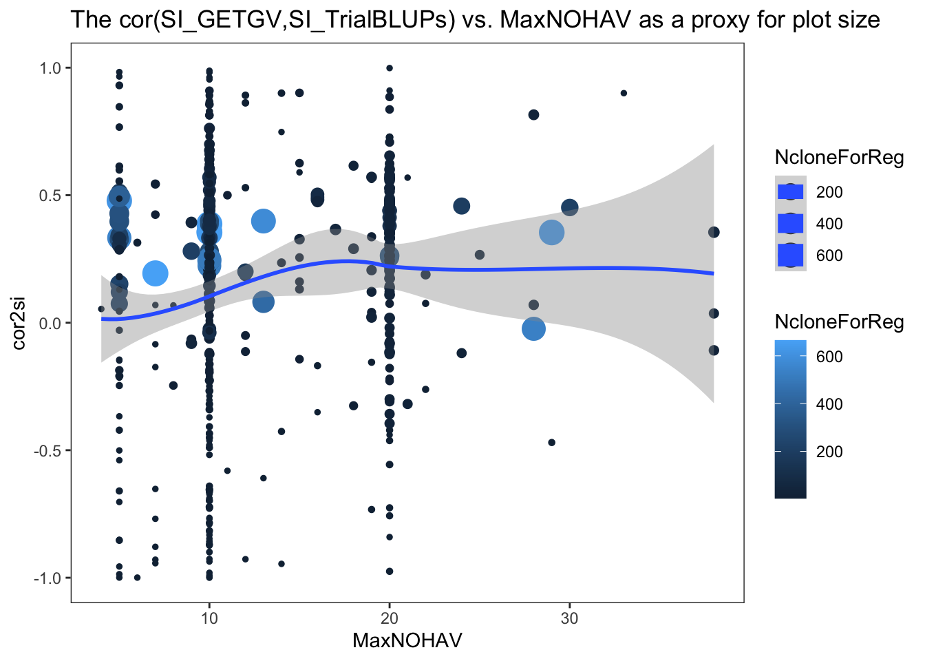
| Version | Author | Date |
|---|---|---|
| 3a1faa0 | wolfemd | 2021-07-14 |
estSelError %>%
  filter(NcloneForReg>=5) %>%
  ggplot(.,aes(x=MaxNOHAV,y=TrialMSE,color=NcloneForReg,size=NcloneForReg)) +
  geom_point() + geom_smooth() + theme_bw() + theme(panel.grid = element_blank()) +
  labs(title = "Trial-specific selection error ests. vs. MaxNOHAV",
       subtitle = "NcloneForReg>=5")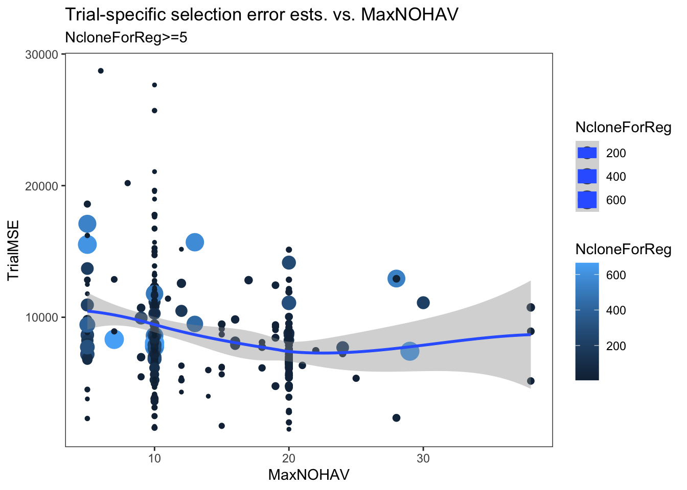
| Version | Author | Date |
|---|---|---|
| 3a1faa0 | wolfemd | 2021-07-14 |
estSelError %>%
  filter(NcloneForReg>=10,
         cor2si>=0) %>%
  ggplot(.,aes(x=MaxNOHAV,y=TrialMSE)) +
  geom_point() + geom_smooth() + theme_bw() + theme(panel.grid = element_blank()) +
  labs(title = "Trial-specific selection error ests. vs. MaxNOHAV",
       subtitle = "Trials with Positive 'cor2si'. NcloneForReg>=10 and cor2si>=0")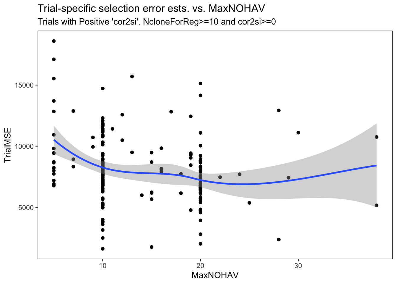
| Version | Author | Date |
|---|---|---|
| 3a1faa0 | wolfemd | 2021-07-14 |
estSelError %>%
  filter(NcloneForReg>=5) %>%
  ggplot(.,aes(x=cut_width(MaxNOHAV,5),y=TrialMSE)) +
  geom_boxplot() + theme_bw() + theme(panel.grid = element_blank()) +
  labs(title = "Trial-specific selection error ests. vs. MaxNOHAV",
       subtitle = "NcloneForReg>=5",
       xlab = "Binned MaxNOHAV")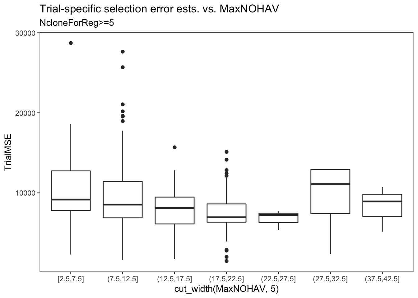
| Version | Author | Date |
|---|---|---|
| 3a1faa0 | wolfemd | 2021-07-14 |
estSelError %>%
  filter(NcloneForReg>=10,
         cor2si>=0.2) %>%
  ggplot(.,aes(x=cut_width(MaxNOHAV,5),y=TrialMSE)) +
  geom_boxplot() + theme_bw() + theme(panel.grid = element_blank()) +
  labs(title = "Trial-specific selection error ests. vs. MaxNOHAV",
       subtitle = "NcloneForReg>=10 and cor2si>=0.2",
       xlab = "Binned MaxNOHAV")
| Version | Author | Date |
|---|---|---|
| 3a1faa0 | wolfemd | 2021-07-14 |
estSelError %>%
  filter(NcloneForReg>=5) %>%
  ggplot(.,aes(x=MaxNOHAV,y=1-r2_si,size=NcloneForReg,color=NcloneForReg)) +
  geom_point() + geom_smooth(method = 'lm') + geom_smooth(color='red')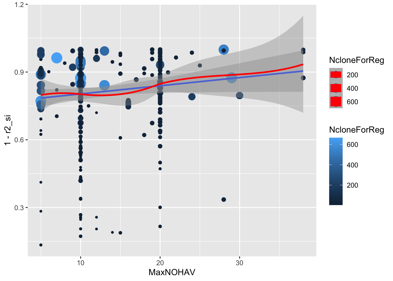
| Version | Author | Date |
|---|---|---|
| 3a1faa0 | wolfemd | 2021-07-14 |
estSelError %>%
  filter(NcloneForReg>5) %>%
  ggplot(.,aes(x=r2_si,y=cor2si,size=NcloneForReg,color=NcloneForReg)) +
  geom_point()
| Version | Author | Date |
|---|---|---|
| 3a1faa0 | wolfemd | 2021-07-14 |
estSelError %>%
  filter(NcloneForReg>=5) %>%
  ggplot(.,aes(x=cor2si,y=TrialMSE,size=NcloneForReg,color=NcloneForReg)) +
  geom_point()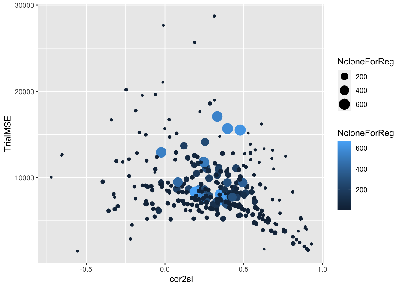
| Version | Author | Date |
|---|---|---|
| 3a1faa0 | wolfemd | 2021-07-14 |
Regression analysis
Try to measure an effect size of increasing the number of stands per plot.
Regression 1: NcloneForReg>=5
lm(TrialMSE~MaxNOHAV+NcloneForReg,
   data = estSelError %>% filter(NcloneForReg>=5)) %>% summary
Call:
lm(formula = TrialMSE ~ MaxNOHAV + NcloneForReg, data = estSelError %>%
    filter(NcloneForReg >= 5))

Residuals:
    Min      1Q  Median      3Q     Max
-7642.2 -2190.8  -761.5  1465.9 18919.2

Coefficients:
              Estimate Std. Error t value Pr(>|t|)
(Intercept)  10684.412    556.226  19.209  < 2e-16 ***
MaxNOHAV      -148.712     35.886  -4.144 4.42e-05 ***
NcloneForReg     1.790      1.714   1.044    0.297
---
Signif. codes:  0 '***' 0.001 '**' 0.01 '*' 0.05 '.' 0.1 ' ' 1

Residual standard error: 3772 on 305 degrees of freedom
Multiple R-squared:  0.0598,    Adjusted R-squared:  0.05364
F-statistic:   9.7 on 2 and 305 DF,  p-value: 8.239e-05
Regression 2: NcloneForReg>=10, cor2si>=0.2
lm(TrialMSE~MaxNOHAV+NcloneForReg,
   data = estSelError %>% filter(NcloneForReg>=10,
                                 cor2si>=0.2)) %>% summary
Call:
lm(formula = TrialMSE ~ MaxNOHAV + NcloneForReg, data = estSelError %>%
    filter(NcloneForReg >= 10, cor2si >= 0.2))

Residuals:
    Min      1Q  Median      3Q     Max
-6122.2 -1391.3  -176.5  1298.8 10335.9

Coefficients:
             Estimate Std. Error t value Pr(>|t|)
(Intercept)  8606.959    534.561  16.101  < 2e-16 ***
MaxNOHAV      -94.342     32.678  -2.887   0.0044 **
NcloneForReg    5.844      1.332   4.388 2.01e-05 ***
---
Signif. codes:  0 '***' 0.001 '**' 0.01 '*' 0.05 '.' 0.1 ' ' 1

Residual standard error: 2476 on 169 degrees of freedom
Multiple R-squared:  0.1688,    Adjusted R-squared:  0.159
F-statistic: 17.16 on 2 and 169 DF,  p-value: 1.635e-07
sessionInfo()R version 4.1.0 (2021-05-18)
Platform: x86_64-apple-darwin17.0 (64-bit)
Running under: macOS Big Sur 10.16
Matrix products: default
BLAS: /Library/Frameworks/R.framework/Versions/4.1/Resources/lib/libRblas.dylib
LAPACK: /Library/Frameworks/R.framework/Versions/4.1/Resources/lib/libRlapack.dylib
locale:
[1] en_US.UTF-8/en_US.UTF-8/en_US.UTF-8/C/en_US.UTF-8/en_US.UTF-8
attached base packages:
[1] stats graphics grDevices utils datasets methods base
other attached packages:
[1] magrittr_2.0.1 forcats_0.5.1 stringr_1.4.0 dplyr_1.0.7
[5] purrr_0.3.4 readr_1.4.0 tidyr_1.1.3 tibble_3.1.2
[9] ggplot2_3.3.5 tidyverse_1.3.1 workflowr_1.6.2
loaded via a namespace (and not attached):
[1] Rcpp_1.0.7 lattice_0.20-44 lubridate_1.7.10 here_1.0.1
[5] assertthat_0.2.1 rprojroot_2.0.2 digest_0.6.27 utf8_1.2.1
[9] R6_2.5.0 cellranger_1.1.0 backports_1.2.1 reprex_2.0.0
[13] evaluate_0.14 highr_0.9 httr_1.4.2 pillar_1.6.1
[17] rlang_0.4.11 readxl_1.3.1 rstudioapi_0.13 whisker_0.4
[21] jquerylib_0.1.4 Matrix_1.3-4 rmarkdown_2.9 labeling_0.4.2
[25] splines_4.1.0 munsell_0.5.0 broom_0.7.8 compiler_4.1.0
[29] httpuv_1.6.1 modelr_0.1.8 xfun_0.24 pkgconfig_2.0.3
[33] mgcv_1.8-36 htmltools_0.5.1.1 tidyselect_1.1.1 viridisLite_0.4.0
[37] fansi_0.5.0 crayon_1.4.1 dbplyr_2.1.1 withr_2.4.2
[41] later_1.2.0 grid_4.1.0 nlme_3.1-152 jsonlite_1.7.2
[45] gtable_0.3.0 lifecycle_1.0.0 DBI_1.1.1 git2r_0.28.0
[49] scales_1.1.1 cli_3.0.0 stringi_1.6.2 farver_2.1.0
[53] fs_1.5.0 promises_1.2.0.1 xml2_1.3.2 bslib_0.2.5.1
[57] ellipsis_0.3.2 generics_0.1.0 vctrs_0.3.8 tools_4.1.0
[61] glue_1.4.2 hms_1.1.0 yaml_2.2.1 colorspace_2.0-2
[65] rvest_1.0.0 knitr_1.33 haven_2.4.1 sass_0.4.0