CUT&Tag Data Processing and Analysis Tutorial

workflowr

• Summary
• Checks
• Past versions

Last updated: 2020-06-01

Checks: 6 1

Knit directory: CUTTag_tutorial/

This reproducible R Markdown analysis was created with workflowr (version 1.6.2). The Checks tab describes the reproducibility checks that were applied when the results were created. The Past versions tab lists the development history.

---

R Markdown file: up-to-date

Great! Since the R Markdown file has been committed to the Git repository, you know the exact version of the code that produced these results.

Environment: empty

Great job! The global environment was empty. Objects defined in the global environment can affect the analysis in your R Markdown file in unknown ways. For reproduciblity it’s best to always run the code in an empty environment.

Seed: set.seed(20200415)

The command set.seed(20200415) was run prior to running the code in the R Markdown file. Setting a seed ensures that any results that rely on randomness, e.g. subsampling or permutations, are reproducible.

Session information: recorded

Great job! Recording the operating system, R version, and package versions is critical for reproducibility.

Cache: none

Nice! There were no cached chunks for this analysis, so you can be confident that you successfully produced the results during this run.

File paths: absolute

Using absolute paths to the files within your workflowr project makes it difficult for you and others to run your code on a different machine. Change the absolute path(s) below to the suggested relative path(s) to make your code more reproducible.

absolute	relative
/fh/fast/gottardo_r/yezheng_working/cuttag/CUTTag_tutorial	.

Repository version: 99a8aa3

Great! You are using Git for version control. Tracking code development and connecting the code version to the results is critical for reproducibility.

The results in this page were generated with repository version 99a8aa3. See the Past versions tab to see a history of the changes made to the R Markdown and HTML files.

Note that you need to be careful to ensure that all relevant files for the analysis have been committed to Git prior to generating the results (you can use wflow_publish or wflow_git_commit). workflowr only checks the R Markdown file, but you know if there are other scripts or data files that it depends on. Below is the status of the Git repository when the results were generated:

Ignored files:
    Ignored:    .DS_Store
    Ignored:    .Rhistory
    Ignored:    .Rproj.user/
    Ignored:    analysis/.DS_Store

Untracked files:
    Untracked:  ._.DS_Store
    Untracked:  alignment/
    Untracked:  analysis/._.DS_Store
    Untracked:  analysis/figures/
    Untracked:  analysis/pipeline.sh
    Untracked:  analysis/pipeline.sh~
    Untracked:  analysis/pipeline2.sh
    Untracked:  analysis/pipeline2.sh~
    Untracked:  analysis/qhKZSPchYbXQn.auc.bed
    Untracked:  analysis/tutorials.Rmd~
    Untracked:  data/IgG_rep1/
    Untracked:  data/IgG_rep2/
    Untracked:  data/K27me3_rep1/
    Untracked:  data/K27me3_rep2/
    Untracked:  data/K4me3_rep1/
    Untracked:  data/K4me3_rep2/
    Untracked:  data/hg38_gene/
    Untracked:  fastq/
    Untracked:  fastqFileQC/
    Untracked:  peakCalling/

Note that any generated files, e.g. HTML, png, CSS, etc., are not included in this status report because it is ok for generated content to have uncommitted changes.

---

These are the previous versions of the repository in which changes were made to the R Markdown (analysis/index.Rmd) and HTML (docs/index.html) files. If you’ve configured a remote Git repository (see ?wflow_git_remote), click on the hyperlinks in the table below to view the files as they were in that past version.

File	Version	Author	Date	Message
html	8db752d	yezhengSTAT	2020-06-01	Build site.
Rmd	cbd9c8c	yezhengSTAT	2020-06-01	Publish the initial files for myproject
html	2e55365	yezhengSTAT	2020-06-01	Build site.
html	d544756	yezhengSTAT	2020-06-01	Build site.
Rmd	d37def8	yezhengSTAT	2020-04-15	Start workflowr project.

---

contact: yzheng23@fredhutch.org

File creation: March 13, 2020

Final Update: May 31, 2020

Approximate time: 60 - 120 minutes

I. Introduction

1.1. Overview of CUT&Tag

Cleavage Under Targets and Tagmentation (CUT&Tag) is an epigenomic profiling strategy in which antibodies are bound to chromatin proteins in situ in permeabilized nuclei, and then used to tether the cut-and-paste transposase Tn5. Activation of the transposase simultaneously cleaves DNA and adds DNA sequencing adapters (“tagmentation”) for paired-end DNA sequencing. The most recent streamlined CUT&Tag protocol has successfully suppressed exposure artifacts to ensure high-fidelity mapping of the antibody-targeted protein and improved signal-to-noise over current chromatin profiling methods. Streamlined CUT&Tag can be performed in a single PCR tube from cells to amplified libraries, providing low-cost high-resolution genome-wide chromatin maps. By simplifying library preparation, CUT&Tag requires less than a day at the bench from live cells to sequencing-ready barcoded libraries. Because of low background levels, barcoded and pooled CUT&Tag libraries can be sequenced for ~$25 per sample, enabling routine genome-wide profiling of chromatin proteins and modifications that requires no special skills or equipment.

The mapping of chromatin features genome-wide has traditionally been performed using chromatin immunoprecipitation (ChIP), in which chromatin is cross-linked and solubilized and an antibody to a protein or modification of interest is used to immunoprecipitate the bound DNA. Very little has changed in the way ChIP is most generally performed since it was first described 35 years ago, and remains fraught with signal-to-noise issues and artifacts. An alternative chromatin profiling strategy is enzyme tethering in situ whereby the chromatin protein or modification of interest is targeted by an antibody or fusion protein, and the underlying DNA is marked or released. A succession of enzyme-tethering methods have been introduced over the past two decades. Cleavage Under Targets & Tagmentation (CUT&Tag) is a tethering method that uses a protein-A-Tn5 (pA-Tn5) transposome fusion protein. Permeabilized cells or nuclei are incubated with antibody to a specified chromatin protein, and then pA-Tn5 loaded with mosaic end adaptors is successively tethered to antibody-bound sites. Activation of the transposome by adding magnesium ions results in the integration of the adaptors into nearby DNA. These are then amplified to generate sequencing libraries. Antibody-tethered Tn5-based methods achieve high sensitivity owing to stringent washing of samples after pA-Tn5 tethering and the high efficiency of adaptor integration. The improved signal-to-noise relative to ChIP-seq translates to an order-of-magnitude reduction in the amount of sequencing required to map chromatin features. Therefore, we use barcoded PCR primers to enable sample-pooling (typically up to 90 samples) for paired-end sequencing on Illumina NGS sequencers.

With all the differences between ChIP-seq and CUT&Tag data, we launched this tutorial tailored for processing and analyzing CUT&Tag data.

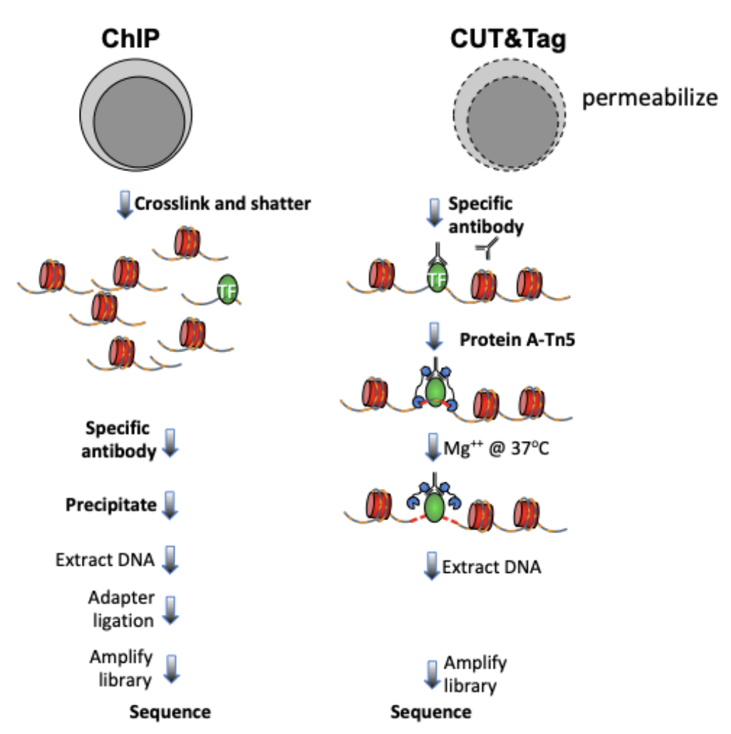
Figure 1. Differences between immunoprecipitation and in antibody-targeted chromatin profiling strategies.

1.2. Objectives

This tutorial is designed for processing and analyzing CUT&Tag data following the Bench top CUT&Tag V.3 protocol, an enzyme-tethering strategy that provides efficient high-resolution sequencing libraries for profiling diverse chromatin components.

1.3. Requirements

• Linux system

• R (versions >= 3.6)
  • dplyr
  • stringr
  • ggplot2
  • viridis
  • GenomicRanges
  • chromVAR
  • DESeq2
  • ChIPseqSpikeInFree

• FastQC(version >= 0.11.9)

• Bowtie2 (version >= 2.3.4.3)

• samtools (version >= 1.10)

• bedtools (version >= 2.29.1)

• Picard (version >= 2.18.29)

• SEACR (version >= 1.3)

• deepTools (version >= 2.0)

1.4. Data

In this tutorial, we use data from Kaya-Okur et al. (2020).

• H3K27me3:
  • SH_Hs_K27m3_NX_0918 as replicate 1
  • SH_Hs_K27m3_Xpc_0107 as replicate 2
• H3K4me3:
  • SH_Hs_K4m3_NX_0918 as replicate 1
  • SH_Hs_K4m3_Xpc_0107 as replicate 2
• IgG:
  • SH_Hs_IgG_o_2kA_0919 as replicate 1
  • SH_Hs_IgG_n_6kA_0918 as replicate 2

1.5. Download the data

We will do the data downloading, pre-processing and processing on each histone sample respectively. In this tutorial, we will use H3K27me3 replicate 1 as the illustration.

First, we need to denote the histone name and project path.

##== linux command ==##
histName="K27me3_rep1"
projPath="/path/to/project/where/data/and/results/are/saved"

Data were downloaded from http://heniweb.fhcrc.org/data/hs20190927_SH.html.

##== linux command ==##
mkdir -p $projPath/data
wget -P $projPath/data path/to/open/source/data

II. Data Pre-processing

2.1. Merge technical replicate if needed [Optional]

##== linux command ==##
mkdir -p ${projPath}/fastq
cat ${projPath}/data/${histName}/*_R1_*.fastq.gz >${projPath}/fastq/${histName}_R1.fastq.gz
cat ${projPath}/data/${histName}/*_R2_*.fastq.gz >${projPath}/fastq/${histName}_R2.fastq.gz

2.2. Quality Control using FastQC [Optional]

2.2.1 Obtain FastQC

##== linux command ==##
mkdir -p $projPath/tools
wget -P $projPath/tools https://www.bioinformatics.babraham.ac.uk/projects/fastqc/fastqc_v0.11.9.zip
cd $projPath/tools
unzip fastqc_v0.11.9.zip

2.2.2 Run FastQC for quality check

##== linux command ==##
mkdir -p ${projPath}/fastqFileQC/${histName}

$projPath/tools/FastQC/fastqc -o ${projPath}/fastqFileQC/${histName} -f fastq ${projPath}/fastq/${histName}_R1.fastq.gz
$projPath/tools/FastQC/fastqc -o ${projPath}/fastqFileQC/${histName} -f fastq ${projPath}/fastq/${histName}_R2.fastq.gz

2.2.3 Intepret the quality check results.

Quality check reference: https://www.bioinformatics.babraham.ac.uk/projects/fastqc/bad_sequence_fastqc.html

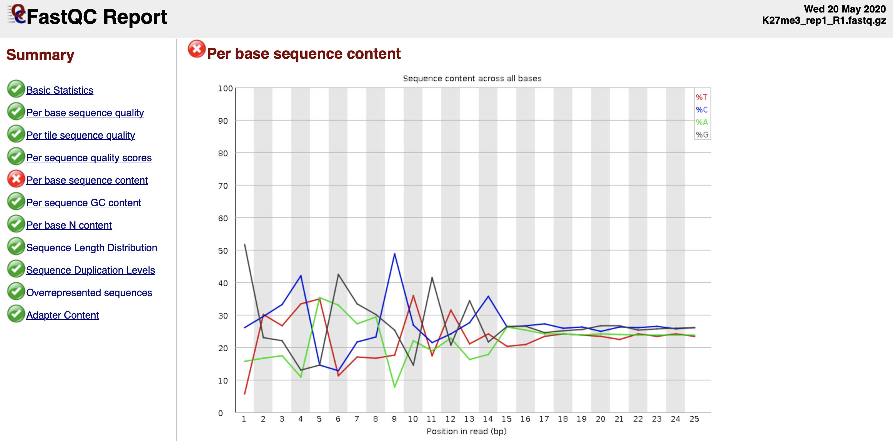
Figure 2. Per base sequence content fails the FastQC quality check.

?? - Tn5 preference

• The discordant sequence content at the begining of the reads are common phenomenon for CUT&Tag reads. What you might be detecting is the 10-bp periodicity that shows up as a sawtooth pattern in the length distribution. If so, this is normal and will not affect alignment or peak calling. In any case we do not recommend trimming as the bowtie2 parameters that we list will give accurate mapping information without trimming.

III. Alignment

3.1. Bowtie2 alignment [required]

##== linux command ==##
cores=8
ref="/path/to/bowtie2Index/hg38"

mkdir -p ${projPath}/alignment/sam/bowtie2_summary
mkdir -p ${projPath}/alignment/bam
mkdir -p ${projPath}/alignment/bed
mkdir -p ${projPath}/alignment/bedgraph

## Build the bowtie2 reference genome index if needed:
## bowtie2-build path/to/hg38/fasta/hg38.fa /path/to/bowtie2Index/hg38

bowtie2 --end-to-end --very-sensitive --no-mixed --no-discordant --phred33 -I 10 -X 700 -p ${cores} -x ${ref} -1 ${projPath}/fastq/${histName}_R1.fastq.gz -2 ${projPath}/fastq/${histName}_R2.fastq.gz -S ${projPath}/alignment/sam/${histName}_bowtie2.sam &> ${projPath}/alignment/sam/bowtie2_summary/${histName}_bowtie2.txt

The paired-end reads are aligned by Bowtie2 using parameters: --end-to-end --very-sensitive --no-mixed --no-discordant --phred33 -I 10 -X 700

Parameters explanation:

http://bowtie-bio.sourceforge.net/bowtie2/manual.shtml

Bowtie2 alignment results summary is saved at ${projPath}/alignment/sam/bowtie2)summary/${histName}_bowtie2.txt:

2984630 reads; of these:
  2984630 (100.00%) were paired; of these:
    125110 (4.19%) aligned concordantly 0 times
    2360430 (79.09%) aligned concordantly exactly 1 time
    499090 (16.72%) aligned concordantly >1 times
95.81% overall alignment rate

• 2984640 is the sequencing depth, i.e., total number of paired reads.
• 125110 is the number of read pairs that fail to be mapped.
• 2360430 + 499090 is the number of read paris that are successfully mapped.
• 95.81% is the overall alignment rate

3.1.1 Sequencing depth

We first check the sequencing depth of the data we have.

##=== R command ===## 
## Path to the project and histone list
projPath = "/fh/fast/gottardo_r/yezheng_working/cuttag/CUTTag_tutorial"
histList = c("K27me3_rep1", "K27me3_rep2", "K4me3_rep1", "K4me3_rep2", "IgG_rep1", "IgG_rep2")

## Collect the alignment results from the bowtie2 alignment summary files
alignResult = c()
for(hist in histList){
  alignRes = read.table(paste0(projPath, "/alignment/sam/bowtie2_summary/", hist, "_bowtie2.txt"), header = FALSE, fill = TRUE)
  alignRate = substr(alignRes$V1[6], 1, nchar(as.character(alignRes$V1[6]))-1)
  histInfo = strsplit(hist, "_")[[1]]
  alignResult = data.frame(seqDepth = alignRes$V1[1] %>% as.character %>% as.numeric, alignNum = alignRes$V1[4] %>% as.character %>% as.numeric + alignRes$V1[5] %>% as.character %>% as.numeric, alignRate = alignRate %>% as.numeric, Histone = histInfo[1], Replicate = histInfo[2])  %>% rbind(alignResult, .)
}

## Generate sequencing depth boxplot
alignResult %>% ggplot(aes(x = Histone, y = seqDepth, fill = Histone)) +
    geom_boxplot() +
    geom_jitter(aes(color = Replicate), position = position_jitter(0.15)) +
    scale_fill_viridis(discrete = TRUE, begin = 0.1, end = 0.9, option = "magma", alpha = 0.8) +
    scale_color_viridis(discrete = TRUE, begin = 0.1, end = 0.9) +
    theme_bw(base_size = 20) +
    ylab("Sequencing Depth") +
    xlab("")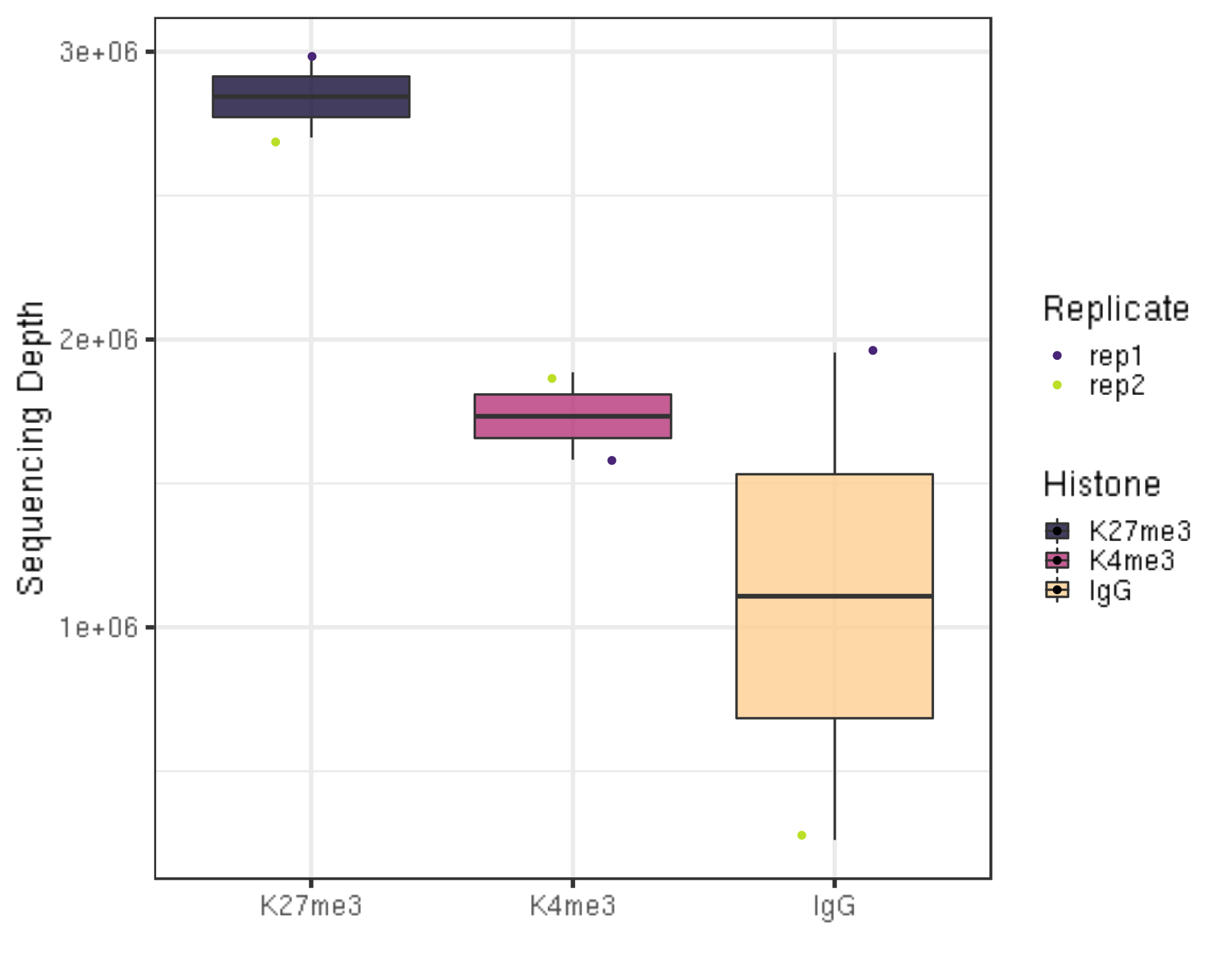

Past versions of unnamed-chunk-8-1.png

Version	Author	Date
8db752d	yezhengSTAT	2020-06-01

• Millions of reads are collected for the illustration data.
• A reasonable minimum sequencing depth is ??

3.1.2 Alignemnt rate

One aspect to check the quality of the data is to look at the alignment rate.

##=== R command ===## 
alignResult %>% ggplot(aes(x = Histone, y = alignRate, fill = Histone)) +
    geom_boxplot() +
    geom_jitter(aes(color = Replicate), position = position_jitter(0.15)) +
    scale_fill_viridis(discrete = TRUE, begin = 0.1, end = 0.9, option = "magma", alpha = 0.8) +
    scale_color_viridis(discrete = TRUE, begin = 0.1, end = 0.9) +
    theme_bw(base_size = 20) +
    ylab("% of Mapped Fragments") +
    xlab("")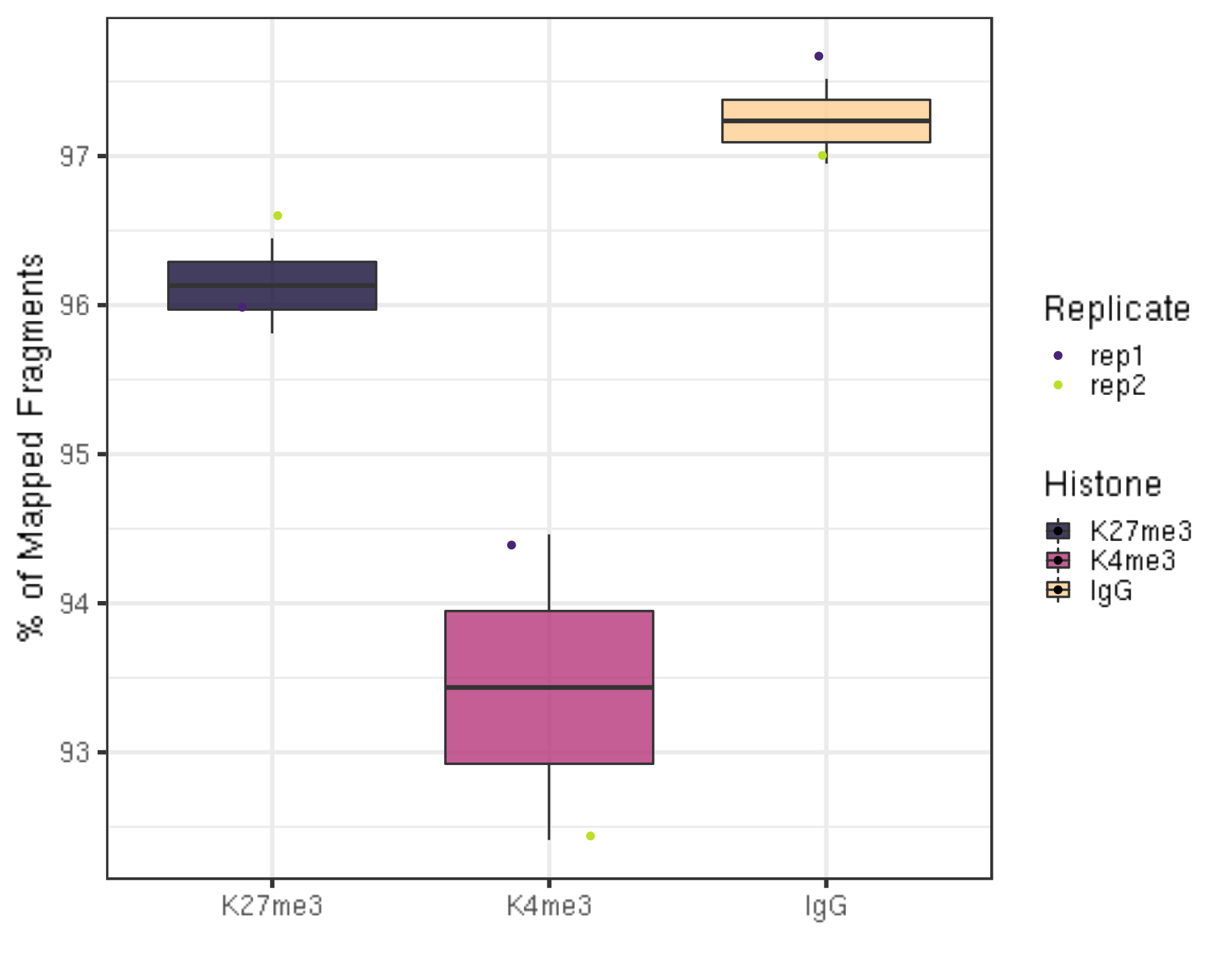

Past versions of unnamed-chunk-9-1.png

Version	Author	Date
8db752d	yezhengSTAT	2020-06-01

• The alignment rates are all above 90% which is pretty high.

3.1.3 Number of alignable reads

After alignment, we can check the number of mapped reads, i.e., valid sequencing depth for downstream analysis.

##=== R command ===## 
alignResult %>% ggplot(aes(x = Histone, y = alignNum, fill = Histone)) +
    geom_boxplot() +
    geom_jitter(aes(color = Replicate), position = position_jitter(0.15)) +
    scale_fill_viridis(discrete = TRUE, begin = 0.1, end = 0.9, option = "magma", alpha = 0.8) +
    scale_color_viridis(discrete = TRUE, begin = 0.1, end = 0.9) +
    theme_bw(base_size = 20) +
    ylab("# of Mapped Fragments") +
    xlab("")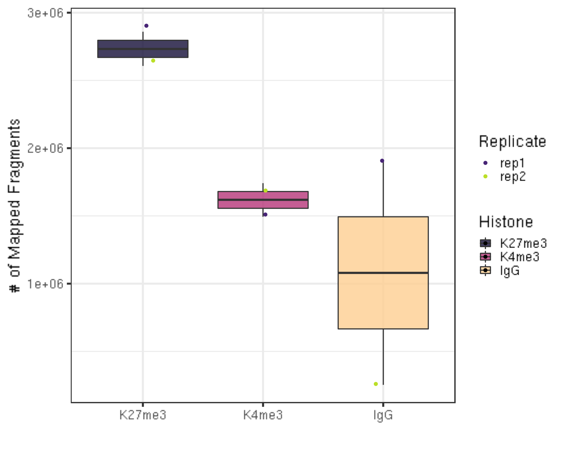

Past versions of unnamed-chunk-10-1.png

Version	Author	Date
8db752d	yezhengSTAT	2020-06-01

• There are still millions of reads that are alignable and pass on to downstream analysis.

3.2. Filtering mapped reads by the mapping quality filtering [optinal]

Some project may require more stringent filtering on the alignment quality score. This blog detailedly discussed how does bowtie assign quality score with examples.

MAPQ(x) = -10 * \(log_{10}\)(P(x is mapped wrongly)) = -10 * \(log_{10}(p)\)

which ranges from 0 to 37, 40 or 42.

samtools view -q minQualityScore will eliminate all the alignment results that are below the minQualityScore defined by user.

##== linux command ==##
minQualityScore=2
samtools view -q $minQualityScore ${projPath}/alignment/sam/${histName}_bowtie2.sam >${projPath}/alignment/sam/${histName}_bowtie2.qualityScore$minQualityScore.sam

• If you do implement this filtering, please replace the following input sam file into this filtered sam file.

3.3. Remove duplicates [optional/required]

• CUT&Tag uses the antibody-tethered Tn5-based methods that can achieve high sensitivity, hence the resulting background noise is low and signal regions are enriched and narrow. Therefore, theoretically we may collect fragments that share exactly the same starting and ending sequences which are not because of the PCR duplication.

• Practically, we found for high quality and high sequencing depth samples, the duplication rate is pretty low and the rest duplicated fragments are highly likely to be the true enrichment signals. Thus, for these sample, we do not recommend removing the duplicates.

• However, for samples that are of low quality and have too few sequencing depth, their duplication rate can be super high. We recommend removing the duplicates for these samples.

• The following commands show how to check the duplication rate using Picard.

##== linux command ==##
## depending on how you load picard and your server environment, the picardCMD can be different. Adjust accordingly.
picardCMD="java -jar picard.jar"
mkdir -p $projPath/alignment/rmDuplicate/picard_summary

## Sort by coordinate
$picardCMD SortSam I=$projPath/alignment/sam/${histName}_bowtie2.sam O=$projPath/alignment/sam/${histName}_bowtie2.sorted.sam SORT_ORDER=coordinate

## mark duplicates
$picardCMD MarkDuplicates I=$projPath/alignment/sam/${histName}_bowtie2.sorted.sam O=$projPath/alignment/removeDuplicate/${histName}_bowtie2.sorted.dupMarked.sam METRICS_FILE=$projPath/alignment/removeDuplicate/picard_summary/${histName}_picard.dupMark.txt

## remove duplicates
picardCMD MarkDuplicates I=$projPath/alignment/sam/${histName}_bowtie2.sorted.sam O=$projPath/alignment/removeDuplicate/${histName}_bowtie2.sorted.rmDup.sam REMOVE_DUPLICATES=true METRICS_FILE=$projPath/alignment/removeDuplicate/picard_summary/${histName}_picard.rmDup.txt

3.3.1 Duplication rate

First, we summarize the duplication rate.

##=== R command ===## 
## Summarize the duplication information from the picard summary outputs.
dupResult = c()
for(hist in histList){
  dupRes = read.table(paste0(projPath, "/alignment/rmDuplicate/picard_summary/", hist, "_picard.rmDup.txt"), header = TRUE, fill = TRUE)
  
  histInfo = strsplit(hist, "_")[[1]]
  dupResult = data.frame(mappedN = dupRes$READ_PAIRS_EXAMINED[1] %>% as.character %>% as.numeric, dupRate = dupRes$PERCENT_DUPLICATION[1] %>% as.character %>% as.numeric, Histone = histInfo[1], Replicate = histInfo[2]) %>% mutate(uniqN = mappedN * (1-dupRate))  %>% rbind(dupResult, .)
}

## generate boxplot figure for the  duplication rate
dupResult %>% ggplot(aes(x = Histone, y = dupRate * 100, fill = Histone)) +
    geom_boxplot() +
    geom_jitter(aes(color = Replicate), position = position_jitter(0.15)) +
    scale_fill_viridis(discrete = TRUE, begin = 0.1, end = 0.9, option = "magma", alpha = 0.8) +
    scale_color_viridis(discrete = TRUE, begin = 0.1, end = 0.9) +
    theme_bw(base_size = 20) +
    ylab("Duplication Rate (*100%)") +
    xlab("")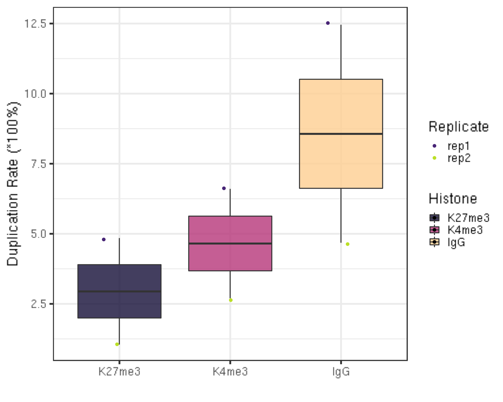

Past versions of unnamed-chunk-13-1.png

Version	Author	Date
8db752d	yezhengSTAT	2020-06-01

• If you go back to the sequencing depth figure in section 1.1 and 1.3, you will find the negative correlation between the sequencing depth and the duplication rate. In other words, usually samples that have higher sequencing depth will have low duplication rate.

3.3.2 Unique library size

Next, we check the unique library size without duplications.

##=== R command ===## 
dupResult %>% ggplot(aes(x = Histone, y = uniqN, fill = Histone)) +
    geom_boxplot() +
    geom_jitter(aes(color = Replicate), position = position_jitter(0.15)) +
    scale_fill_viridis(discrete = TRUE, begin = 0.1, end = 0.9, option = "magma", alpha = 0.8) +
    scale_color_viridis(discrete = TRUE, begin = 0.1, end = 0.9) +
    theme_bw(base_size = 20) +
    ylab("# of Unique Fragments") +
    xlab("")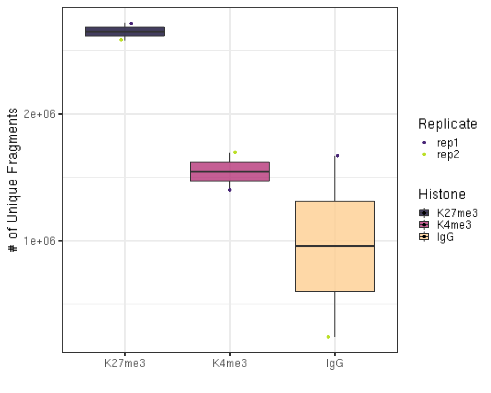

Past versions of unnamed-chunk-14-1.png

Version	Author	Date
8db752d	yezhengSTAT	2020-06-01

• We still have millions of unique fragments left.

3.4. Assess mapped fragment size distribution [Required]

##== linux command ==##
mkdir -p $projPath/alignment/sam/fragmentLen

## Extract the 9th column from the alignment sam file which is the fragment length
samtools view -F 0x04 $projPath/alignment/sam/${histName}_bowtie2.sam | awk -F'\t' 'function abs(x){return ((x < 0.0) ? -x : x)} {print abs($9)}' | sort | uniq -c | awk -v OFS="\t" '{print $2, $1/2}' >$projPath/alignment/sam/fragmentLen/${histName}_fragmentLen.txt

##=== R command ===## 
## Collect the fragment size information
fragLen = c()
for(hist in histList){
  histInfo = strsplit(hist, "_")[[1]]
  fragLen = read.table(paste0(projPath, "/alignment/sam/fragmentLen/", hist, "_fragmentLen.txt"), header = FALSE) %>% mutate(fragLen = V1 %>% as.numeric, Weight = as.numeric(V2)/sum(as.numeric(V2)), Histone = histInfo[1], Replicate = histInfo[2], histInfo = hist) %>% rbind(fragLen, .)
  
}

## Generate the fragment size density plot (violin plot)
fragLen %>% ggplot(aes(x = histInfo, y = fragLen, weight = Weight, fill = Histone)) +
    geom_violin(bw = 5) +
    scale_y_continuous(breaks = seq(0, 800, 50)) +
    scale_fill_viridis(discrete = TRUE, begin = 0.1, end = 0.9, option = "magma", alpha = 0.8) +
    scale_color_viridis(discrete = TRUE, begin = 0.1, end = 0.9) +
    theme_bw(base_size = 20) +
    ggpubr::rotate_x_text(angle = 20) +
    ylab("Fragment Length") +
    xlab("")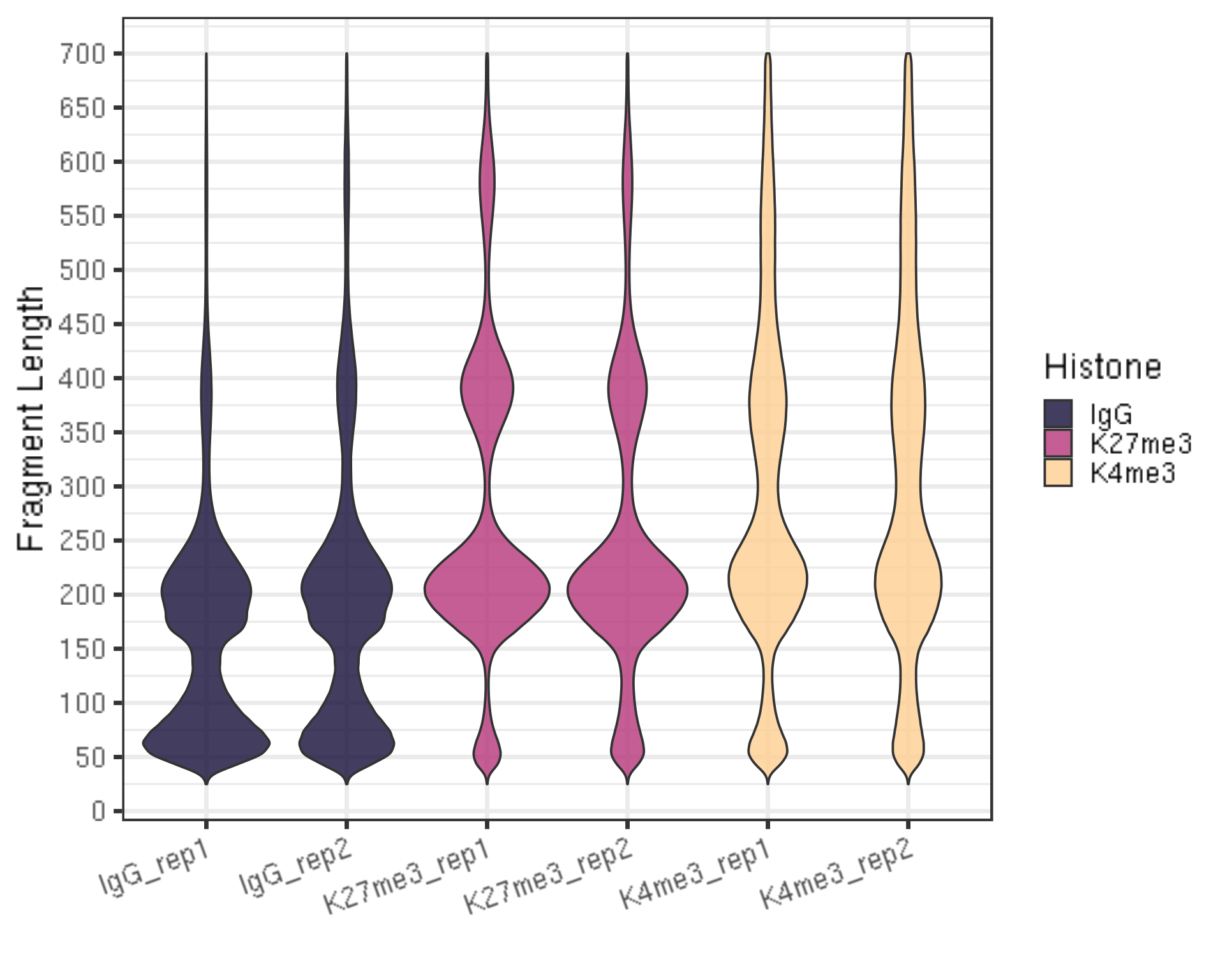

Past versions of unnamed-chunk-16-1.png

Version	Author	Date
8db752d	yezhengSTAT	2020-06-01

• There should be periodic peaking pattern of 200bp as a unit.
• These are fragments that are the size of nucleosomes, the expected result of targeting histone.
• The smaller fragments (50-100 bp) are not bad, they just result from tagmentation within nucleosomes.

IV. Alignment results filtering and file format conversion

This section is required in preparation for the peak calling and visualization where there are a few filtering and file format conversion that need to be done.

##== linux command ==##
## Filter and keep the mapped read pairs
samtools view -bS -F 0x04 $projPath/alignment/sam/${histName}_bowtie2.sam $projPath/alignment/bam/${histName}_bowtie2.mapped.bam

## Convert into bed file format
bedtools bamtobed -i $projPath/alignment/bam/${histName}_bowtie2.mapped.bam -bedpe $projPath/alignment/bed/${histName}_bowtie2.bed

## Keep the read pairs that are on the same chromosome and fragment length less than 1000bp.
awk '$1==$4 && $6-$2 < 1000 {print $0}' $projPath/alignment/bed/${histName}_bowtie2.bed $projPath/alignment/bed/${histName}_bowtie2.clean.bed

## Only extract the fragment related columns
cut -f 1,2,6 $projPath/alignment/bed/${histName}_bowtie2.clean.bed | sort -k1,1 -k2,2n -k3,3n  >$projPath/alignment/bed/${histName}_bowtie2.fragments.bed

V. Spike-in calibration

This section is optional but recommended depending on your experimental protocol.

5.1 Alignment to the spike-in genome [optional/recommended]

• To calibrate samples in a series for samples done in parallel using the same antibody we use counts of E. coli fragments carried over with the pA-Tn5 the same as one would for an ordinary spike-in.

• We align E. coli carry-over fragments to the NCBI Ecoli genome (Escherichia coli str. K12 substr. MG1655 U00096.3) with --no-overlap --no-dovetail options (```–end-to-end –very-sensitive –no-overlap –no-dovetail –no-mixed –no-discordant –phred33 -I 10 -X 700````) to avoid possible cross-mapping of the experimental genome to that of the carry-over E. coli DNA that is used for calibration.

##== linux command ==##
spikeInRef="/shared/ngs/illumina/henikoff/Bowtie2/Ecoli"
chromSize="/fh/fast/gottardo_r/yezheng_working/SupplementaryData/hg38/chromSize/hg38.chrom.size"

## bowtie2-build path/to/Ecoli/fasta/Ecoli.fa /path/to/bowtie2Index/Ecoli
bowtie2 --end-to-end --very-sensitive --no-mixed --no-discordant --phred33 -I 10 -X 700 -p ${cores} -x ${spikeInRef} -1 ${projPath}/fastq/${histName}_R1.fastq.gz -2 ${projPath}/fastq/${histName}_R2.fastq.gz -S $projPath/alignment/sam/${histName}_bowtie2_spikeIn.sam &> $projPath/alignment/sam/bowtie2_summary/${histName}_bowtie2_spikeIn.txt

seqDepthDouble=`samtools view -F 0x04 seqDepth=$((seqDepthDouble/2))
echo $seqDepth >$projPath/alignment/sam/bowtie2_summary/${histName}_bowtie2_spikeIn.seqDepth


if [[ "$seqDepth" -gt "1" ]]; then
    
    mkdir -p $projPath/alignment/bedgraph

    scale_factor=`echo "10000 / $seqDepth" | bc -l`
    echo "Scaling factor for $histName is: $scale_factor!"
    bedtools genomecov -bg -scale $scale_factor -i $projPath/alignment/bed/${histName}_bowtie2.fragments.bed -g $chromSize > $projPath/alignment/bedgraph/${histName}_bowtie2.fragments.normalized.bedgraph
    
fi

5.2 Spike-in alignment rate

##=== R command ===## 
spikeAlign = c()
for(hist in histList){
  spikeRes = read.table(paste0(projPath, "/alignment/sam/bowtie2_summary/", hist, "_bowtie2_spikeIn.txt"), header = FALSE, fill = TRUE)
  alignRate = substr(spikeRes$V1[6], 1, nchar(as.character(spikeRes$V1[6]))-1)
  histInfo = strsplit(hist, "_")[[1]]
  spikeAlign = data.frame(seqDepth = spikeRes$V1[1] %>% as.character %>% as.numeric, alignNum = spikeRes$V1[4] %>% as.character %>% as.numeric + spikeRes$V1[5] %>% as.character %>% as.numeric, alignRate = alignRate %>% as.numeric, Histone = histInfo[1], Replicate = histInfo[2])  %>% rbind(spikeAlign, .)
}

## Generate alignment rate boxplot
spikeAlign %>% ggplot(aes(x = Histone, y = alignRate, fill = Histone)) +
    geom_boxplot() +
    geom_jitter(aes(color = Replicate), position = position_jitter(0.15)) +
    scale_fill_viridis(discrete = TRUE, begin = 0.1, end = 0.9, option = "magma", alpha = 0.8) +
    scale_color_viridis(discrete = TRUE, begin = 0.1, end = 0.9) +
    theme_bw(base_size = 20) +
    ylab("Spike-in Alignment Rate") +
    xlab("")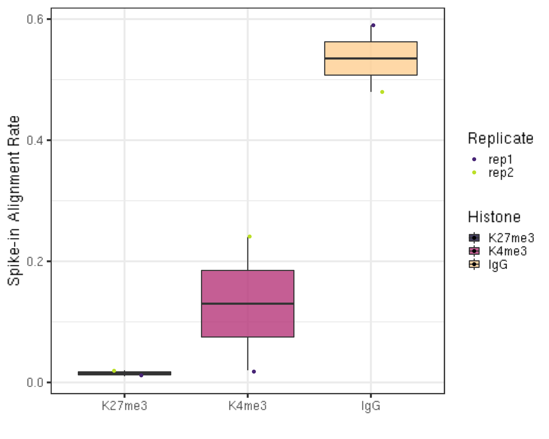

Past versions of unnamed-chunk-19-1.png

Version	Author	Date
8db752d	yezhengSTAT	2020-06-01

• The percentage of reads mapped to E.coli depends on the number of cells and how broadly distributed the antibody epitope is. Based on our normal exploratory experiments, usually, this percentage range from 0.01% to 11.5%.
• Especially for IgG, this percentage is usually much higher (2%-11.5%) than the histone modification.
• For even wilder exploratory experiments, we found using a few thousand or even a few hundreds of cells, and this number can soar to 30% or even 70%. However, the percentage drops back to 4% using 65k cells.

5.3 Scaling factor

The scaling factor is defined to be

Scaling_factor = Scale multiplier/ (Total # of fragments mapped to spike-in genome)

##=== R command ===## 
scaleFactor = c()
multiplier = 10000
for(hist in histList){
  spikeDepth = read.table(paste0(projPath, "/alignment/sam/bowtie2_summary/", hist, "_bowtie2_spikeIn.seqDepth"), header = FALSE, fill = TRUE)$V1[1]
  
  histInfo = strsplit(hist, "_")[[1]]
  scaleFactor = data.frame(scaleFactor = multiplier/spikeDepth, Histone = histInfo[1], Replicate = histInfo[2])  %>% rbind(scaleFactor, .)
}

## Generate sequencing depth boxplot
scaleFactor %>% ggplot(aes(x = Histone, y = scaleFactor, fill = Histone)) +
    geom_boxplot() +
    geom_jitter(aes(color = Replicate), position = position_jitter(0.15)) +
    scale_fill_viridis(discrete = TRUE, begin = 0.1, end = 0.9, option = "magma", alpha = 0.8) +
    scale_color_viridis(discrete = TRUE, begin = 0.1, end = 0.9) +
    theme_bw(base_size = 20) +
    ylab("Spike-in Scalling Factor") +
    xlab("")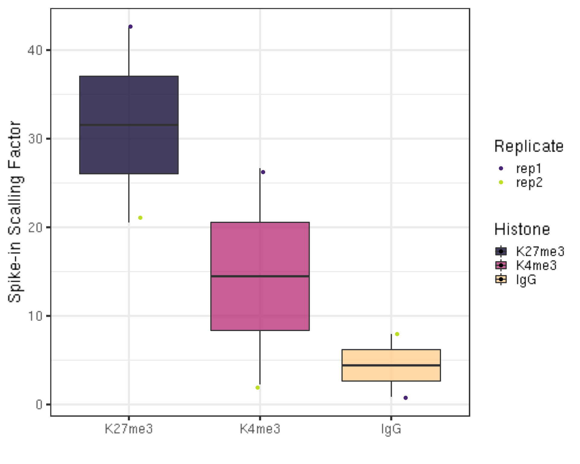

Past versions of unnamed-chunk-20-1.png

Version	Author	Date
8db752d	yezhengSTAT	2020-06-01

• There is actually no universal scale factor that can be used on different samples. Instead, the key idea of calibration is

  (primary_genome_mapped_count_at_bp) * Scaling_factor =

  (primary_genome_mapped_count_at_bp) * Scale multiplier / (spike-in_genome_total_of_mapped_fragments)

• The underlying assumption is that the primary # genome to spike-in genome ratio per cell is expected to be the same for all samples that use the same number of cells in an experiment comparing treatment.

• The “scale multiplier” in the above formula can be an arbitrary multiplier (e.g., 10000) to avoid small fractions.

• The drop of file size should be expected as the input files are the alignment for all the fragments but the output is genome coverage which is like a summary of the fragment alignment results. However, it won’t hurt to carefully check the output file.

5.4 Total number of fragments after normaliztion (seqDepth)

##=== R command ===## 
normDepth = inner_join(scaleFactor, alignResult, by = c("Histone", "Replicate")) %>% mutate(normDepth = alignNum * scaleFactor)

normDepth %>% ggplot(aes(x = Histone, y = normDepth, fill = Histone)) +
    geom_boxplot() +
    geom_jitter(aes(color = Replicate), position = position_jitter(0.15)) +
    scale_fill_viridis(discrete = TRUE, begin = 0.1, end = 0.9, option = "magma", alpha = 0.8) +
    scale_color_viridis(discrete = TRUE, begin = 0.1, end = 0.9) +
    theme_bw(base_size = 20) +
    ylab("Total number of fragments after normalization") +
    xlab("") + 
    coord_cartesian(ylim = c(1000000, 130000000))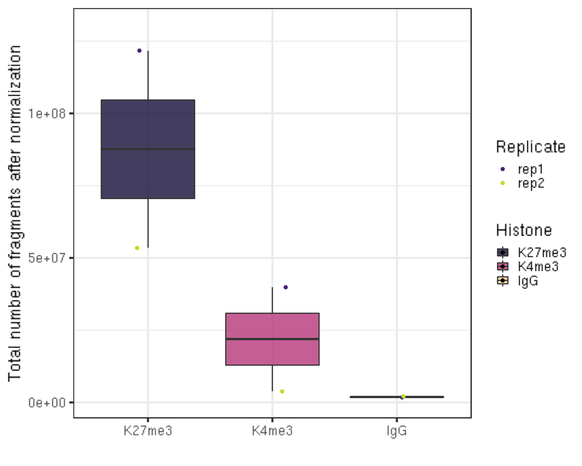

Past versions of unnamed-chunk-21-1.png

Version	Author	Date
8db752d	yezhengSTAT	2020-06-01

5.5 ChIPseqSpikeInFree for experiments without spike-ins [Optional]

ChIPseqSpikeInFree: a ChIP-seq normalization approach to reveal global changes in histone modifications without spike-in is a novel ChIP-seq normalization method to effectively determine scaling factors for samples across various conditions and treatments, which does not rely on exogenous spike-in chromatin or peak detection to reveal global changes in histone modification occupancy. The installation details can be found on github.

##=== R command ===## 
library("ChIPseqSpikeInFree")

bamDir = paste0(projPath, "/alignment/bam")
metaData = c()
for(hist in histList){
  histInfo = strsplit(hist, "_")[[1]] 

  metaData = data.frame(ID = paste0(hist, "_bowtie2.mapped.bam"), ANTIBODY = histInfo[1], GROUP = histInfo[2]) %>% rbind(metaData, .)
  
}
write.table(metaData, file = paste0(projPath, "/alignment/ChIPseqSpikeInFree/metaData.txt"), row.names = FALSE, quote = FALSE, sep = "\t")

metaFile = paste0(projPath, "/alignment/ChIPseqSpikeInFree/metaData.txt")
bams = paste0(projPath, "/alignment/bam/", metaData$ID)
ChIPseqSpikeInFree(bamFiles = bams, chromFile = "hg38", metaFile = metaFile, prefix = paste0(projPath, "/alignment/ChIPseqSpikeInFree/SpikeInFree_results"))

• Interpretation of the ChIPseqSpikeInFree output.

• How to use ChIPseqSpikeInFree scaling factor.

VI. Peak calling

6.1. SEACR

The usage manual of SEACR can be found here. We have calibrated the fragment frequency with respect to the spike-in, therefore for field 3, we can set the normalization option to be “non”. Otherwise, “norm” is recommended.

##== linux command ==##
seacr="/fh/fast/gottardo_r/yezheng_working/Software/SEACR/SEACR_1.3.sh"
histControl=$2
mkdir -p $projPath/peakCalling/SEACR

bash $seacr $projPath/alignment/bedgraph/${histName}_bowtie2.fragments.normalized.bedgraph \
     $projPath/alignment/bedgraph/${histControl}_bowtie2.fragments.normalized.bedgraph \
     non stringent $projPath/peakCalling/SEACR/${histName}_seacr_control.peaks

bash $seacr $projPath/alignment/bedgraph/${histName}_bowtie2.fragments.normalized.bedgraph 0.01 non stringent $projPath/peakCalling/SEACR/${histName}_seacr_top0.01.peaks

6.1.1 Number of peaks called

##=== R command ===## 
peakN = c()
peakWidth = c()
peakType = c("control", "top0.01")
for(hist in histList){
  histInfo = strsplit(hist, "_")[[1]]
  if(histInfo[1] != "IgG"){
    for(type in peakType){
      peakInfo = read.table(paste0(projPath, "/peakCalling/SEACR/", hist, "_seacr_", type, ".peaks.stringent.bed"), header = FALSE, fill = TRUE)  %>% mutate(width = abs(V3-V2))
      peakN = data.frame(peakN = nrow(peakInfo), peakType = type, Histone = histInfo[1], Replicate = histInfo[2]) %>% rbind(peakN, .)
      peakWidth = data.frame(width = peakInfo$width, peakType = type, Histone = histInfo[1], Replicate = histInfo[2])  %>% rbind(peakWidth, .)
    }
  }
}

peakN %>% ggplot(aes(x = Histone, y = peakN, fill = Histone)) +
    geom_boxplot() +
    geom_jitter(aes(color = Replicate), position = position_jitter(0.15)) +
    facet_grid(~peakType) +
    scale_fill_viridis(discrete = TRUE, begin = 0.1, end = 0.9, option = "magma", alpha = 0.8) +
    scale_color_viridis(discrete = TRUE, begin = 0.1, end = 0.9) +
    theme_bw(base_size = 20) +
    ylab("Number of Peaks") +
    xlab("")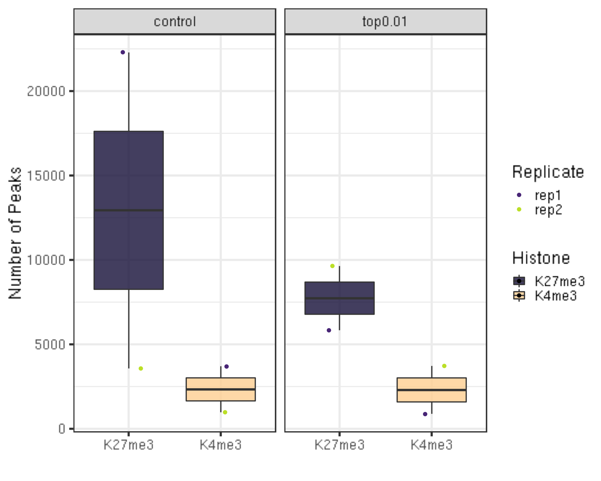

Past versions of unnamed-chunk-24-1.png

Version	Author	Date
8db752d	yezhengSTAT	2020-06-01

6.1.2 Distribution of the peak length

##=== R command ===## 
peakWidth %>% ggplot(aes(x = Histone, y = width, fill = Histone)) +
    geom_violin() +
    facet_grid(Replicate~peakType) +
    scale_fill_viridis(discrete = TRUE, begin = 0.1, end = 0.9, option = "magma", alpha = 0.8) +
    scale_color_viridis(discrete = TRUE, begin = 0.1, end = 0.9) +
    theme_bw(base_size = 20) +
    ylab("Width of Peaks") +
    xlab("")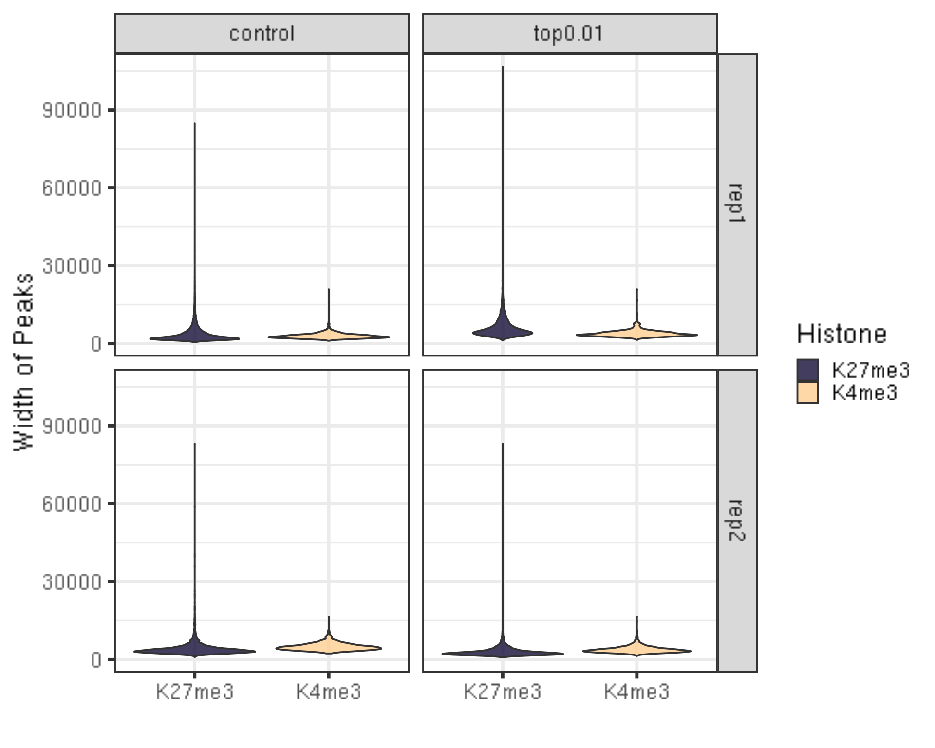

Past versions of unnamed-chunk-25-1.png

Version	Author	Date
8db752d	yezhengSTAT	2020-06-01

##=== R command ===## 
peakWidth %>% ggplot(aes(x = Histone, y = width, fill = Histone)) +
    geom_violin() +
    facet_grid(Replicate~peakType) +
    scale_fill_viridis(discrete = TRUE, begin = 0.1, end = 0.9, option = "magma", alpha = 0.8) +
    scale_color_viridis(discrete = TRUE, begin = 0.1, end = 0.9) +
    theme_bw(base_size = 20) +
    ylab("Width of Peaks") +
    xlab("") +
    coord_cartesian(ylim = c(0, 25000))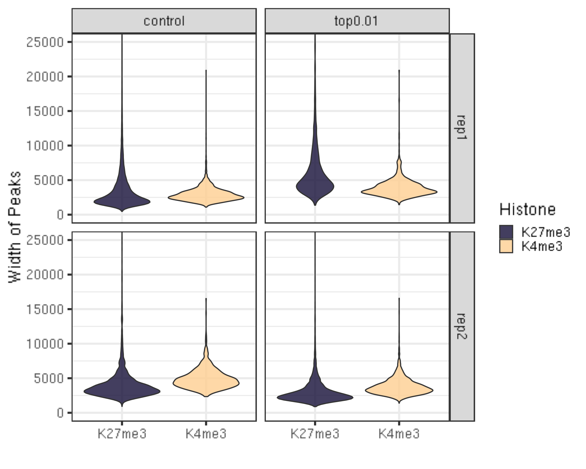

Past versions of unnamed-chunk-26-1.png

Version	Author	Date
8db752d	yezhengSTAT	2020-06-01

6.1.3 Reproducibility of the peak across biological replicates

##=== R command ===## 
histL = c("K27me3", "K4me3")
repL = paste0("rep", 1:2)
peakType = c("control", "top0.01")
peakOverlap = c()
for(type in peakType){
  for(hist in histL){
    overlap.gr = GRanges()
    for(rep in repL){
      peakInfo = read.table(paste0(projPath, "/peakCalling/SEACR/", hist, "_", rep, "_seacr_", type, ".peaks.stringent.bed"), header = FALSE, fill = TRUE)
      peakInfo.gr = GRanges(peakInfo$V1, IRanges(start = peakInfo$V2, end = peakInfo$V3), strand = "*")
      if(length(overlap.gr) >0){
        overlap.gr = overlap.gr[findOverlaps(overlap.gr, peakInfo.gr)@from]
      }else{
        overlap.gr = peakInfo.gr
        
      }
    }
    peakOverlap = data.frame(peakReprod = length(overlap.gr), Histone = hist, peakType = type) %>% rbind(peakOverlap, .)
  }
}

peakReprod = left_join(peakN, peakOverlap, by = c("Histone", "peakType")) %>% mutate(peakReprodRate = peakReprod/peakN * 100)

peakReprod %>% ggplot(aes(x = Histone, y = peakReprodRate, fill = Histone, label = round(peakReprodRate, 2))) +
    geom_bar(stat = "identity") +
    geom_text(vjust = 0.1) +
    facet_grid(Replicate~peakType) +
    scale_fill_viridis(discrete = TRUE, begin = 0.1, end = 0.9, option = "magma", alpha = 0.8) +
    scale_color_viridis(discrete = TRUE, begin = 0.1, end = 0.9) +
    theme_bw(base_size = 20) +
    ylab("% of Peaks Reproduced across Biological Replicate") +
    xlab("")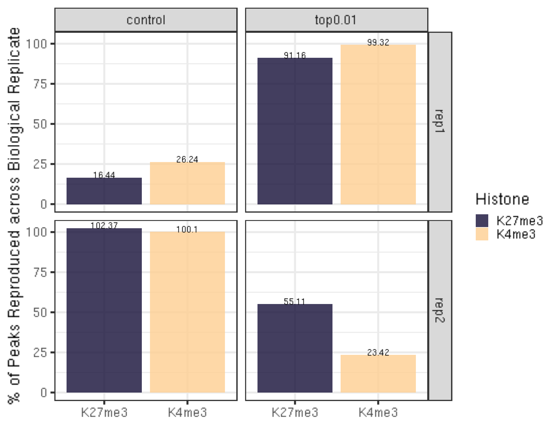

Past versions of unnamed-chunk-27-1.png

Version	Author	Date
8db752d	yezhengSTAT	2020-06-01

6.1.4 FRagment proportion in Peaks regions (FRiPs).

• We utilize the SEACR peaks contrasting with IgG controls for illustration.

##=== R command ===## 
library(chromVAR)

bamDir = paste0(projPath, "/alignment/bam")
inPeakData = c()
## overlap with bam file to get count
for(hist in histL){
  for(rep in repL){
    peakRes = read.table(paste0(projPath, "/peakCalling/SEACR/", hist, "_", rep, "_seacr_control.peaks.stringent.bed"), header = FALSE, fill = TRUE)
    peak.gr = GRanges(seqnames = peakRes$V1, IRanges(start = peakRes$V2, end = peakRes$V3), strand = "*")
    bamFile = paste0(bamDir, "/", hist, "_", rep, "_bowtie2.mapped.bam")
    fragment_counts <- getCounts(bamFile, peak.gr, paired = TRUE, by_rg = FALSE, format = "bam")
    inPeakN = counts(fragment_counts)[,1] %>% sum
    inPeakData = rbind(inPeakData, data.frame(inPeakN = inPeakN, Histone = hist, Replicate = rep))
  }
}

frip = left_join(inPeakData, alignResult, by = c("Histone", "Replicate")) %>% mutate(frip = inPeakN/alignNum * 100)

frip %>% ggplot(aes(x = Histone, y = frip, fill = Histone, label = round(frip, 2))) +
    geom_boxplot() +
    geom_jitter(aes(color = Replicate), position = position_jitter(0.15)) +
    scale_fill_viridis(discrete = TRUE, begin = 0.1, end = 0.9, option = "magma", alpha = 0.8) +
    scale_color_viridis(discrete = TRUE, begin = 0.1, end = 0.9) +
    theme_bw(base_size = 20) +
    ylab("% of Fragments in Peaks") +
    xlab("")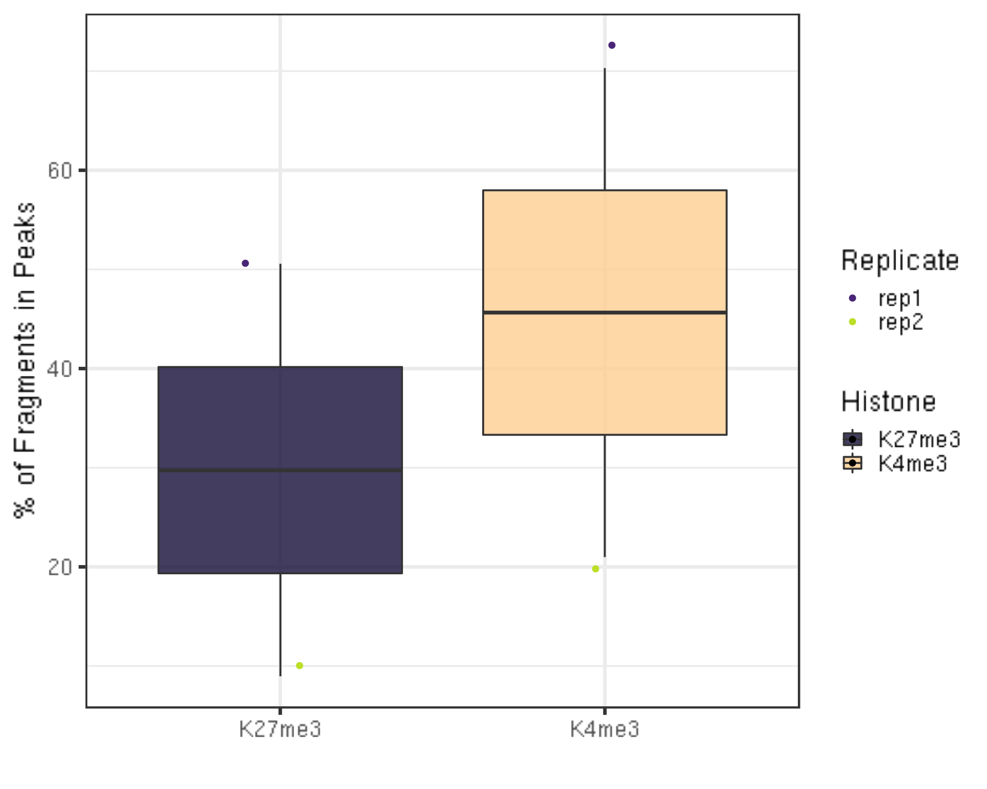

Past versions of unnamed-chunk-28-1.png

Version	Author	Date
8db752d	yezhengSTAT	2020-06-01

6.2. Other peak calling methods.

6.2.1 MACS2: Model-based Analysis of ChIP-Seq (MACS). Installation details can be found here.

##== linux command ==##
histName="K27me3"
controlName="IgG"

mkdir -p $projPath/peakCalling
macs2 callpeak -t ${projPath}/alignment/bam/${histName}_rep1_bowtie2.mapped.bam \
      -c ${projPath}/alignment/bam/${controlName}_rep1_bowtie2.mapped.bam \
      -g hs -f BAMPE -n macs2_peak_q0.1 --outdir $projPath/peakCalling/MACS2 -q 0.1 --keep-dup all 2>${projPath}/peakCalling/MACS2/macs2Peak_summary.txt

6.2.2 Other peak calling methods that are widely used for ChIP-seq data may also be utilized.

• dPeak: dPeak: High Resolution Identification of Transcription Factor Binding Sites from PET and SET ChIP-Seq Data

• MOSAiCS: A Statistical Framework for the Analysis of ChIP-Seq Data

VII. Visualization

• Integrative Genomic Viewer provides web app version and local desktop version. Easy to use.

• UCSC Genome Browser provides the most comprehensive supplementary genome information.

7.1. Browser display of bedgraph files after spike-in calibration.

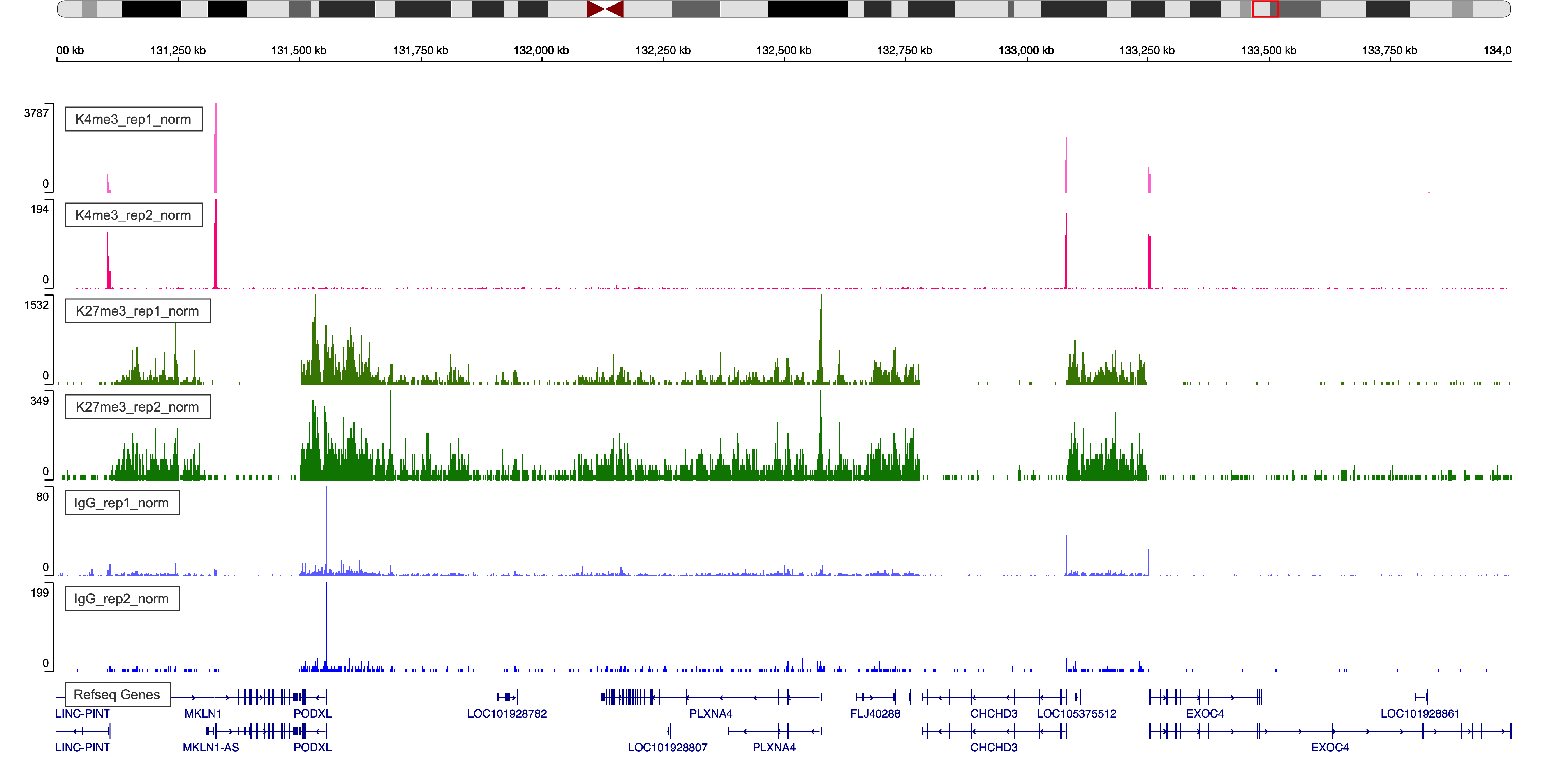
Figure 4. IgV Web Visualization around region chr7:131,000,000-134,000,000

• Check pericentromeric regions that contain lots of repeats are a good place to look since signal will naturally be enriched there for all antibody and IgG data.

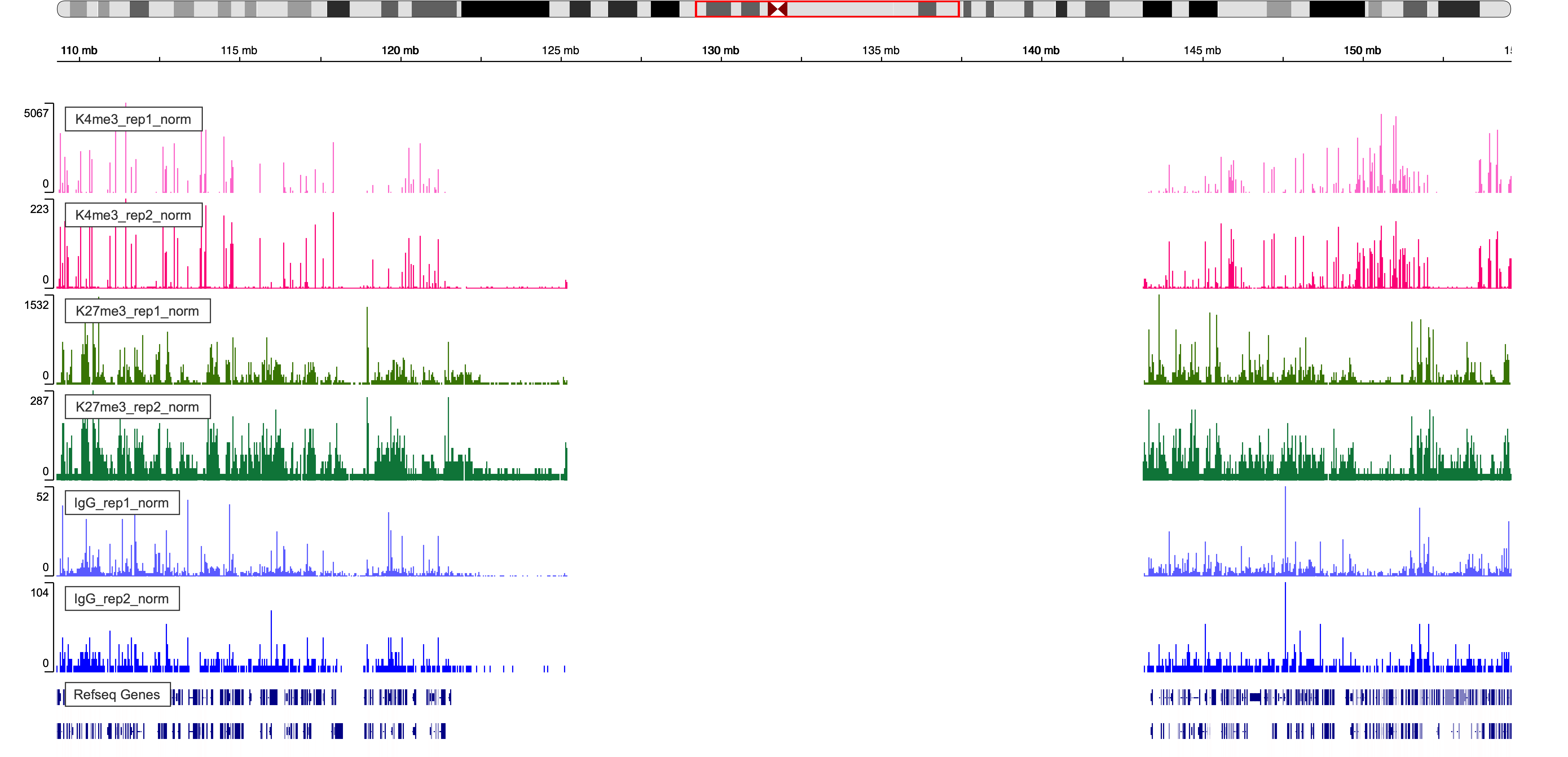
Figure 5. IgV Web Visualization around chr1 pericentromeric region

7.2. Heatmap visualization on specific regions

We will use the computeMatrix and plotHeatmap functions from deepTools to generate the heatmap.

##== linux command ==##
mkdir -p $projPath/alignment/bigwig                                                                                                                                        
samtools sort -o $projPath/alignment/bam/${histName}.sorted.bam $projPath/alignment/bam/${histName}_bowtie2.mapped.bam                                                     
samtools index $projPath/alignment/bam/${histName}.sorted.bam                                                                                                              
bamCoverage -b $projPath/alignment/bam/${histName}.sorted.bam -o $projPath/alignment/bigwig/${histName}_raw.bw                                                             

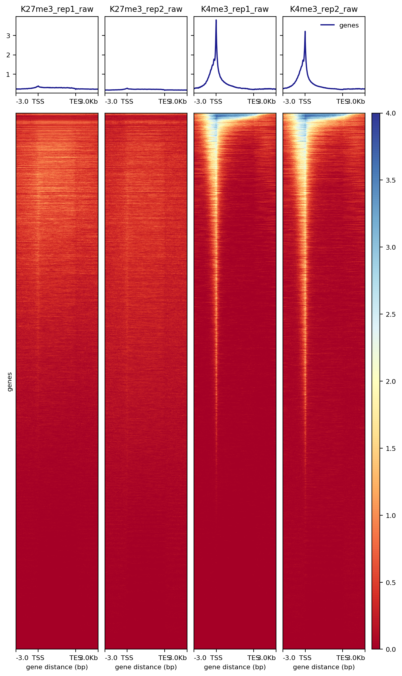
7.2.1 Heatmap over transcripts

##== linux command ==##
cores=8
computeMatrix scale-regions -S $projPath/alignment/bigwig/K27me3_rep1_raw.bw \
                               $projPath/alignment/bigwig/K27me3_rep2_raw.bw \
                               $projPath/alignment/bigwig/K4me3_rep1_raw.bw \
                               $projPath/alignment/bigwig/K4me3_rep2_raw.bw \
                              -R $projPath/data/hg38_gene/hg38_gene.tsv \
                              --beforeRegionStartLength 3000 \
                              --regionBodyLength 5000 \
                              --afterRegionStartLength 3000 \
                              --skipZeros -o $projPath/data/hg38_gene/matrix_gene.mat.gz -p $cores

plotHeatmap -m $projPath/data/hg38_gene/matrix_gene.mat.gz -out $projPath/data/hg38_gene/Histone_gene.png --sortUsing sum

### 7.2.2. Heatmap on CUT&Tag peaks

##== linux command ==##
computeMatrix scale-regions -S $projPath/alignment/bigwig/${histName}_raw.bw \
              -R $projPath/peakCalling/SEACR/${histName}_seacr_control.peaks.stringent.bed \
              --skipZeros -o $projPath/peakCalling/SEACR/${histName}_SEACR.mat.gz -p $cores

plotHeatmap -m $projPath/peakCalling/SEACR/${histName}_SEACR.mat.gz -out $projPath/peakCalling/SEACR/${histName}_SEACR_heatmap.png --sortUsing sum --startLabel "Peak Start" -\
-endLabel "Peak End" --xAxisLabel "" --regionsLabel "Peaks" --samplesLabel ${histName}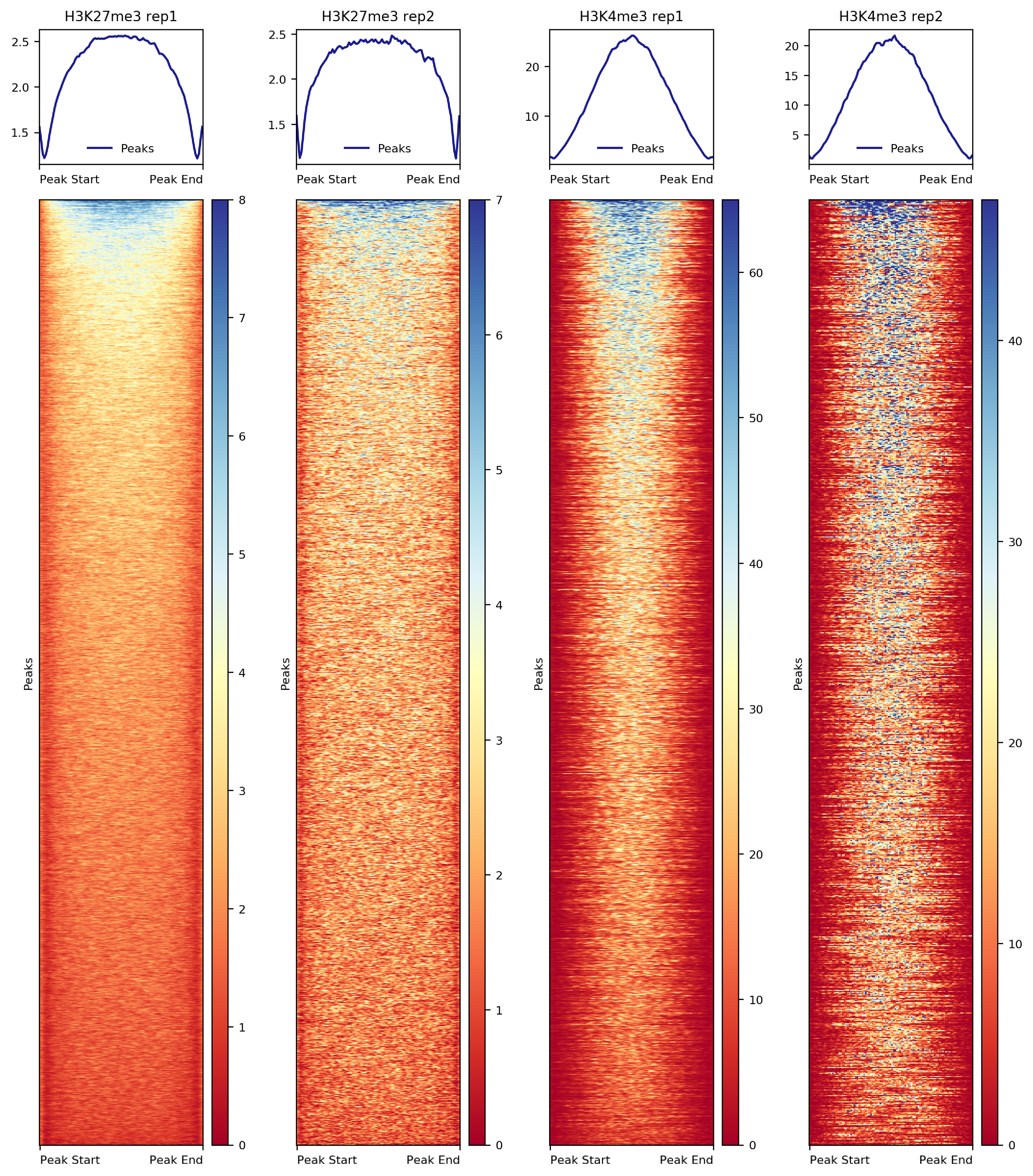

Figure 7. Heatmap of histone enrichment in peaks

VIII. Differential analysis

• DESeq2: Moderated estimation of fold change and dispersion for RNA-seq data with DESeq2

Estimate variance-mean dependence in count data from high-throughput sequencing assays and test for differential expression based on a model using the negative binomial distribution.

• Limma: limma powers differential expression analyses for RNA-sequencing and microarray studies

Limma is an R package for the analysis of gene expression microarray data, especially the use of linear models for analysing designed experiments and the assessment of differential expression. Limma provides the ability to analyse comparisons between many RNA targets simultaneously in arbitrary complicated designed experiments. Empirical Bayesian methods are used to provide stable results even when the number of arrays is small. Limma can be extended to study differential fragment enrichment analysis within peak regions. Notably, limma can deal with both fixed effect model and random effect model.

• edgeR: Differential Expression Analysis of Multifactor RNA-Seq Experiments With Respect to Biological Variation

Differential expression analysis of RNA-seq expression profiles with biological replication. Implements a range of statistical methodology based on the negative binomial distributions, including empirical Bayes estimation, exact tests, generalized linear models and quasi-likelihood tests. As well as RNA-seq, it be applied to differential signal analysis of other types of genomic data that produce read counts, including ChIP-seq, ATAC-seq, Bisulfite-seq, SAGE and CAGE. edgeR can deal with multifactor problem.

8.1. Create the peak x sample matrix.

Usually, the differential tests compare two or more conditions of the same histone modification. In this tutorial, limited by the demonstration data, we will illustrate the differential detection by comparing two replicates of H3K27me3 and two replicates of H3K4me3. We will use DESeq2 (complete tutorial) as illustration.

8.1.1 Create a master peak list merging all the peaks called for each sample.

##=== R command ===## 
mPeak = GRanges()
## overlap with bam file to get count
for(hist in histL){
  for(rep in repL){
    peakRes = read.table(paste0(projPath, "/peakCalling/SEACR/", hist, "_", rep, "_seacr_control.peaks.stringent.bed"), header = FALSE, fill = TRUE)
    mPeak = GRanges(seqnames = peakRes$V1, IRanges(start = peakRes$V2, end = peakRes$V3), strand = "*") %>% append(mPeak, .)
  }
}
masterPeak = reduce(mPeak)

8.1.2 Get the fragment counts for each peak in the master peak list.

##=== R command ===## 
library(DESeq2)
bamDir = paste0(projPath, "/alignment/bam")
countMat = matrix(NA, length(masterPeak), length(histL)*length(repL))
## overlap with bam file to get count
i = 1
for(hist in histL){
  for(rep in repL){
    
    bamFile = paste0(bamDir, "/", hist, "_", rep, "_bowtie2.mapped.bam")
    fragment_counts <- getCounts(bamFile, masterPeak, paired = TRUE, by_rg = FALSE, format = "bam")
    countMat[, i] = counts(fragment_counts)[,1]
    i = i + 1
  }
}
colnames(countMat) = paste(rep(histL, 2), rep(repL, each = 2), sep = "_")

8.2. Sequencing depth normalization and differential enriched peaks detection

##=== R command ===## 
selectR = which(rowSums(countMat) > 5) ## remove low count genes
dataS = countMat[selectR,]
condition = factor(rep(histL, each = length(repL)))
dds = DESeqDataSetFromMatrix(countData = dataS,
                              colData = DataFrame(condition),
                              design = ~ condition)
DDS = DESeq(dds)
normDDS = counts(DDS, normalized = TRUE) ## normalization with respect to the sequencing depth
colnames(normDDS) = paste0(colnames(normDDS), "_norm")
res = results(DDS, independentFiltering = FALSE, altHypothesis = "greaterAbs")

countMatDiff = cbind(dataS, normDDS, res)
head(countMatDiff)

DataFrame with 6 rows and 14 columns
  K27me3_rep1 K4me3_rep1 K27me3_rep2 K4me3_rep2  K27me3_rep1_norm
    <numeric>  <numeric>   <numeric>  <numeric>         <numeric>
1           1          0         242        182 0.124345459941495
2           0          0         175         88                 0
3           0          0         274        194                 0
4         212        130         354        637  26.3612375075969
5           0          2         180        174                 0
6           1          0         193        186 0.124345459941495
    K4me3_rep1_norm K27me3_rep2_norm  K4me3_rep2_norm         baseMean
          <numeric>        <numeric>        <numeric>        <numeric>
1                 0   1642.098979559  860.62486419289 625.712047302957
2                 0 1187.46827034225 416.126307961397 400.898644575912
3                 0 1859.23603470729  917.36936073308 694.151348860094
4  29.5546421781954 2402.07867257804 3012.18702467511 1367.54539423474
5 0.454686802741468 1221.39593520917 822.795199832763 511.161455461169
6                 0 1309.60786386317 879.539696372953 547.317976424015
    log2FoldChange            lfcSE             stat               pvalue
         <numeric>        <numeric>        <numeric>            <numeric>
1 13.9001328992164 1.46237329851921 9.50518784313936  1.9968728862444e-21
2 14.6578324953342 1.58571426872719 9.24367824923438 2.38165977165095e-20
3 15.4521653584048 1.57311982807133 9.82262449603056 8.99701430682874e-23
4 6.59884758504177 0.54558731844186 12.0949431227386 1.12320018631658e-33
5 12.5701262927903 1.12748347918641 11.1488341291359 7.25507086647784e-29
6 13.7045749300893 1.42987365830219 9.58446562779669  9.2937484305191e-22
                  padj
             <numeric>
1 1.76349075171341e-20
2 1.74850821274181e-19
3 1.35404803928629e-21
4 1.47675167643583e-31
5  3.8309051756058e-27
6 9.00551358394595e-21

• DESeq2 requires the input matrix should be un-normalized counts or estimated counts of sequencing reads.

• DESeq2 model internally corrects for library size.

• countMatDiff summarizes the differential analysis results:
  • First 4 columns: raw reads counts after filtering the peak regions with low counts
  • Second 4 columns: normalized read counts eliminating library size difference.
  • Remaining columns: differential detection results.

Conclusion

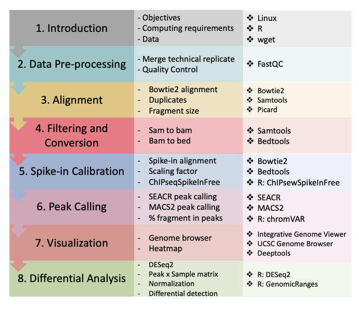
Figure 8. CUT&Tag data processing and analysis.

References

• Citing this tutorial

Kaya-Okur HS, Wu SJ, Codomo CA, Pledger ES, Bryson TD, Henikoff JG, Ahmad K, Henikoff S: CUT&Tag for efficient epigenomic profiling of small samples and single cells. Nature Communications 2019 10:1930 (PMID:31036827).

Session information

sessionInfo()

R version 3.6.2 (2019-12-12)
Platform: x86_64-pc-linux-gnu (64-bit)
Running under: Ubuntu 14.04.5 LTS

Matrix products: default
BLAS/LAPACK: /app/easybuild/software/OpenBLAS/0.2.18-GCC-5.4.0-2.26-LAPACK-3.6.1/lib/libopenblas_prescottp-r0.2.18.so

locale:
 [1] LC_CTYPE=en_US.UTF-8       LC_NUMERIC=C              
 [3] LC_TIME=en_US.UTF-8        LC_COLLATE=en_US.UTF-8    
 [5] LC_MONETARY=en_US.UTF-8    LC_MESSAGES=en_US.UTF-8   
 [7] LC_PAPER=en_US.UTF-8       LC_NAME=C                 
 [9] LC_ADDRESS=C               LC_TELEPHONE=C            
[11] LC_MEASUREMENT=en_US.UTF-8 LC_IDENTIFICATION=C       

attached base packages:
[1] parallel  stats4    stats     graphics  grDevices utils     datasets 
[8] methods   base     

other attached packages:
 [1] DESeq2_1.26.0               SummarizedExperiment_1.16.1
 [3] DelayedArray_0.12.3         BiocParallel_1.20.1        
 [5] matrixStats_0.55.0          Biobase_2.46.0             
 [7] chromVAR_1.8.0              GenomicRanges_1.38.0       
 [9] GenomeInfoDb_1.22.1         IRanges_2.20.2             
[11] S4Vectors_0.24.4            BiocGenerics_0.32.0        
[13] viridis_0.5.1               viridisLite_0.3.0          
[15] ggplot2_3.3.0               stringr_1.4.0              
[17] dplyr_0.8.5                

loaded via a namespace (and not attached):
  [1] readxl_1.3.1                backports_1.1.5            
  [3] Hmisc_4.3-0                 workflowr_1.6.2            
  [5] VGAM_1.1-2                  plyr_1.8.5                 
  [7] lazyeval_0.2.2              splines_3.6.2              
  [9] TFBSTools_1.24.0            digest_0.6.23              
 [11] htmltools_0.4.0             GO.db_3.10.0               
 [13] magrittr_1.5                checkmate_1.9.4            
 [15] memoise_1.1.0               BSgenome_1.54.0            
 [17] cluster_2.1.0               openxlsx_4.1.4             
 [19] Biostrings_2.54.0           readr_1.3.1                
 [21] annotate_1.64.0             R.utils_2.9.2              
 [23] colorspace_1.4-1            blob_1.2.0                 
 [25] haven_2.2.0                 xfun_0.11                  
 [27] crayon_1.3.4                RCurl_1.95-4.12            
 [29] jsonlite_1.6                genefilter_1.68.0          
 [31] TFMPvalue_0.0.8             survival_3.1-8             
 [33] glue_1.3.1                  gtable_0.3.0               
 [35] zlibbioc_1.32.0             XVector_0.26.0             
 [37] car_3.0-5                   abind_1.4-5                
 [39] scales_1.1.0                DBI_1.0.0                  
 [41] rstatix_0.5.0               miniUI_0.1.1.1             
 [43] Rcpp_1.0.3                  xtable_1.8-4               
 [45] htmlTable_1.13.3            foreign_0.8-72             
 [47] bit_1.1-14                  Formula_1.2-3              
 [49] DT_0.10                     htmlwidgets_1.5.1          
 [51] httr_1.4.1                  RColorBrewer_1.1-2         
 [53] acepack_1.4.1               pkgconfig_2.0.3            
 [55] XML_3.98-1.20               R.methodsS3_1.7.1          
 [57] farver_2.0.1                nnet_7.3-12                
 [59] locfit_1.5-9.1              tidyselect_1.0.0           
 [61] labeling_0.3                rlang_0.4.6                
 [63] reshape2_1.4.3              later_1.0.0                
 [65] AnnotationDbi_1.48.0        cellranger_1.1.0           
 [67] munsell_0.5.0               tools_3.6.2                
 [69] DirichletMultinomial_1.28.0 generics_0.0.2             
 [71] RSQLite_2.1.4               broom_0.5.2                
 [73] evaluate_0.14               fastmap_1.0.1              
 [75] yaml_2.2.0                  knitr_1.26                 
 [77] bit64_0.9-7                 fs_1.3.1                   
 [79] zip_2.0.4                   caTools_1.17.1.3           
 [81] purrr_0.3.3                 KEGGREST_1.26.1            
 [83] nlme_3.1-143                whisker_0.4                
 [85] mime_0.7                    R.oo_1.23.0                
 [87] poweRlaw_0.70.6             pracma_2.2.5               
 [89] compiler_3.6.2              rstudioapi_0.10            
 [91] plotly_4.9.1                curl_4.3                   
 [93] png_0.1-7                   ggsignif_0.6.0             
 [95] tibble_2.1.3                geneplotter_1.64.0         
 [97] stringi_1.4.3               highr_0.8                  
 [99] forcats_0.4.0               lattice_0.20-38            
[101] CNEr_1.22.0                 Matrix_1.2-18              
[103] vctrs_0.2.4                 pillar_1.4.2               
[105] lifecycle_0.1.0             data.table_1.12.8          
[107] bitops_1.0-6                httpuv_1.5.2               
[109] rtracklayer_1.46.0          R6_2.4.1                   
[111] latticeExtra_0.6-28         promises_1.1.0             
[113] gridExtra_2.3               rio_0.5.16                 
[115] gtools_3.8.1                assertthat_0.2.1           
[117] seqLogo_1.52.0              rprojroot_1.3-2            
[119] withr_2.1.2                 GenomicAlignments_1.22.1   
[121] Rsamtools_2.2.3             GenomeInfoDbData_1.2.2     
[123] hms_0.5.2                   grid_3.6.2                 
[125] rpart_4.1-15                tidyr_1.0.0                
[127] rmarkdown_1.18              carData_3.0-3              
[129] Cairo_1.5-10                git2r_0.26.1               
[131] ggpubr_0.3.0                shiny_1.4.0                
[133] base64enc_0.1-3