Motif Analysis
Steve Pederson
2022-05-25
Last updated: 2022-05-28
Checks: 6 1
Knit directory:
apocrine_signature_mdamb453/
This reproducible R Markdown analysis was created with workflowr (version 1.7.0). The Checks tab describes the reproducibility checks that were applied when the results were created. The Past versions tab lists the development history.
The R Markdown file has unstaged changes. To know which version of
the R Markdown file created these results, you’ll want to first commit
it to the Git repo. If you’re still working on the analysis, you can
ignore this warning. When you’re finished, you can run
wflow_publish to commit the R Markdown file and build the
HTML.
Great job! The global environment was empty. Objects defined in the global environment can affect the analysis in your R Markdown file in unknown ways. For reproduciblity it’s best to always run the code in an empty environment.
The command set.seed(20220427) was run prior to running
the code in the R Markdown file. Setting a seed ensures that any results
that rely on randomness, e.g. subsampling or permutations, are
reproducible.
Great job! Recording the operating system, R version, and package versions is critical for reproducibility.
Nice! There were no cached chunks for this analysis, so you can be confident that you successfully produced the results during this run.
Great job! Using relative paths to the files within your workflowr project makes it easier to run your code on other machines.
Great! You are using Git for version control. Tracking code development and connecting the code version to the results is critical for reproducibility.
The results in this page were generated with repository version 1bf46f7. See the Past versions tab to see a history of the changes made to the R Markdown and HTML files.
Note that you need to be careful to ensure that all relevant files for
the analysis have been committed to Git prior to generating the results
(you can use wflow_publish or
wflow_git_commit). workflowr only checks the R Markdown
file, but you know if there are other scripts or data files that it
depends on. Below is the status of the Git repository when the results
were generated:
Ignored files:
    Ignored:    .Rhistory
    Ignored:    .Rproj.user/
    Ignored:    analysis/figure/
    Ignored:    analysis/motif_analysis.html
    Ignored:    analysis/site_libs/
    Ignored:    data/bigwig/

Untracked files:
    Untracked:  analysis/motif_analysis.knit.md
    Untracked:  output/all4_h3k27ac.fa
    Untracked:  output/all4_no_h3k27ac.fa
    Untracked:  output/ar_foxa1_gata3_no_tfap2b.fa
    Untracked:  output/ar_foxa1_gata3_tfap2b.fa
    Untracked:  output/meme/

Unstaged changes:
    Modified:   analysis/motif_analysis.Rmd
Note that any generated files, e.g. HTML, png, CSS, etc., are not included in this status report because it is ok for generated content to have uncommitted changes.
These are the previous versions of the repository in which changes were
made to the R Markdown (analysis/motif_analysis.Rmd) and
HTML (docs/motif_analysis.html) files. If you’ve configured
a remote Git repository (see ?wflow_git_remote), click on
the hyperlinks in the table below to view the files as they were in that
past version.
| File | Version | Author | Date | Message |
|---|---|---|---|---|
| Rmd | 1bf46f7 | Steve Pederson | 2022-05-27 | Added motifs distance plots |
| html | 1bf46f7 | Steve Pederson | 2022-05-27 | Added motifs distance plots |
| Rmd | 7cfa8e7 | Steve Pederson | 2022-05-26 | Added TOMTOM |
| html | 7cfa8e7 | Steve Pederson | 2022-05-26 | Added TOMTOM |
| Rmd | 8836090 | Steve Pederson | 2022-05-26 | Added motif centrality |
| html | 8836090 | Steve Pederson | 2022-05-26 | Added motif centrality |
Introduction
This step takes the peaks defined previously and
- Assesses motif enrichment for all ChIP targets within the peaks
- Detect additional binding motifs
As AR is only found bound in the presence of DHT, all peaks are taken using DHT-treatment as the reference condition.
library(memes)
library(universalmotif)
library(tidyverse)
library(plyranges)
library(extraChIPs)
library(rtracklayer)
library(magrittr)
library(BSgenome.Hsapiens.UCSC.hg19)
library(scales)
library(pander)
library(glue)
library(cowplot)
library(parallel)
library(gt)
options(meme_bin = "/opt/meme/bin/")
check_meme_install()
theme_set(theme_bw())
panderOptions("big.mark", ",")getBestMatch <- function(x, subject, min.score = "80%", rc = TRUE, ...) {
pwm <- NULL
if (is.matrix(x)) pwm <- x
if (is(x, "universalmotif")) pwm <- x@motif
stopifnot(!is.null(pwm))
stopifnot(is(subject, "XStringViews"))
matches <- matchPWM(
pwm, subject, min.score = min.score, with.score = TRUE, ...
)
df <- as.data.frame(matches)
df$score <- mcols(matches)$score
df$strand <- "+"
if (rc) {
rc_matches <- matchPWM(
reverseComplement(pwm), subject ,
min.score = min.score, with.score = TRUE,
...
)
rc_df <- as.data.frame(rc_matches)
rc_df$score <- mcols(rc_matches)$score
rc_df$strand <- "-"
df <- bind_rows(df, rc_df)
}
grp_cols <- c("start", "end", "width", "seq", "score")
grp_df <- group_by(df, !!!syms(grp_cols))
summ_df <- summarise(
grp_df, strand = paste(strand, collapse = " "), .groups= "drop"
)
summ_df$strand <- str_replace_all(summ_df$strand, ". .", "*")
summ_df$strand <- factor(summ_df$strand, levels = c("+", "-", "*"))
summ_df$view <- findInterval(summ_df$start, start(subject))
summ_df <- arrange(summ_df, view, desc(score))
best_df <- distinct(summ_df, view, .keep_all = TRUE)
best_df <- mutate(
best_df,
start_in_view = start - start(subject)[view] + 1,
end_in_view = start_in_view + width
)
## This will only be added if the views have names
best_df$view_name <- names(subject[best_df$view])
best_df
}hg19 <- BSgenome.Hsapiens.UCSC.hg19
sq19 <- seqinfo(hg19)all_gr <- here::here("data", "annotations", "all_gr.rds") %>%
read_rds() %>%
lapply(
function(x) {
seqinfo(x) <- sq19
x
}
)
counts <- here::here("data", "rnaseq", "counts.out.gz") %>%
read_tsv(skip = 1) %>%
dplyr::select(Geneid, ends_with("bam")) %>%
dplyr::rename(gene_id = Geneid)
detected <- all_gr$gene %>%
as_tibble() %>%
distinct(gene_id, gene_name) %>%
left_join(counts) %>%
pivot_longer(
cols = ends_with("bam"), names_to = "sample", values_to = "counts"
) %>%
mutate(detected = counts > 0) %>%
group_by(gene_id, gene_name) %>%
summarise(detected = mean(detected) > 0.25, .groups = "drop") %>%
dplyr::filter(detected) %>%
dplyr::select(starts_with("gene"))Pre-existing RNA-seq data was again loaded and the set of 21,173 detected genes was defined as those with \(\geq 1\) aligned read in at least 25% of samples. This dataset represented the DHT response in MDA-MB-453 cells, however, given the existence of both Vehicle and DHT conditions, represents a good representative measure of the polyadenylated components of the transcriptome.
features <- here::here("data", "h3k27ac") %>%
  list.files(full.names = TRUE, pattern = "bed$") %>%
  sapply(import.bed, seqinfo = sq19) %>%
  lapply(granges) %>%
  setNames(basename(names(.))) %>%
  setNames(str_remove_all(names(.), "s.bed")) %>%
  GRangesList() %>%
  unlist() %>%
  names_to_column("feature") %>%
  sort()
The set of H3K27ac-defined features was again used as a marker of regulatory activity, with 16,544 and 15,286 regions defined as enhancers or promoters respectively.
meme_db <- here::here("data", "external", "JASPAR2022_CORE_Hsapiens.meme") %>%
  read_meme() %>%
  to_df() %>%
  as_tibble() %>%
  mutate(
    across(everything(), vctrs::vec_proxy),
    altname = str_remove(altname, "MA[0-9]+\\.[0-9]*\\."),
    organism = "Homo sapiens"
  )
meme_db_detected <- meme_db %>%
  mutate(
    gene_name = str_split(altname, pattern = "::", n = 2)
  ) %>%
  dplyr::filter(
    vapply(
      gene_name,
      function(x) all(x %in% detected$gene_name),
      logical(1)
    )
  )
meme_info <- meme_db_detected %>%
  mutate(motif_length = vapply(motif, function(x){ncol(x@motif)}, integer(1))) %>%
  dplyr::select(name, altname, icscore, motif_length)
The motif database was initially defined as all 727 CORE motifs found in Homo sapiens, as contained in JASPAR2022. In order to minimise irrelevant results, only the 465 motifs associated with a detected gene were then retained.
dht_peaks <- here::here("data", "peaks") %>%
  list.files(recursive = TRUE, pattern = "oracle", full.names = TRUE) %>%
  sapply(read_rds, simplify = FALSE) %>%
  lapply(function(x) x[["DHT"]]) %>%
  lapply(setNames, nm = c()) %>%
  setNames(str_extract_all(names(.), "AR|FOXA1|GATA3|TFAP2B")) %>%
  lapply(
    function(x) {
      seqinfo(x) <- sq19
      x
    }
  )
targets <- names(dht_peaks)
dht_consensus <- dht_peaks %>%
  lapply(granges) %>%
  GRangesList() %>%
  unlist() %>%
  reduce() %>%
  mutate(
    AR = overlapsAny(., dht_peaks$AR),
    FOXA1 = overlapsAny(., dht_peaks$FOXA1),
    GATA3 = overlapsAny(., dht_peaks$GATA3),
    TFAP2B = overlapsAny(., dht_peaks$TFAP2B),
    promoter = bestOverlap(., features, var = "feature", missing = "None") == "promoter",
    enhancer = bestOverlap(., features, var = "feature", missing = "None") == "enhancer",
    H3K27ac = promoter | enhancer
  )
a <- dht_peaks %>%
lapply(mutate, w = width) %>%
lapply(as_tibble) %>%
bind_rows(.id = "target") %>%
ggplot(aes(w, stat(density), colour = target)) +
geom_density() +
scale_x_log10(breaks = c(100, 300, 600, 1e3, 2e3, 3e3), labels = comma) +
labs(
x = "Peak Width (bp)", y = "Density", colour = "Target"
)
b <- dht_peaks %>%
lapply(mutate, w = width) %>%
lapply(as_tibble) %>%
bind_rows(.id = "target") %>%
mutate(skew = 0.5 - peak / w) %>%
ggplot(aes(skew, stat(density), colour = target)) +
geom_density() +
scale_x_continuous(labels = percent) +
labs(
x = "% Width Between Peak Summit and Peak Centre",
y = "Density",
colour = "ChIP Target"
)
plot_grid(
a + theme(legend.position = "none"),
b + theme(legend.position = "none"),
get_legend(b),
rel_widths = c(1, 1, 0.2), nrow = 1,
labels = c("A", "B")
)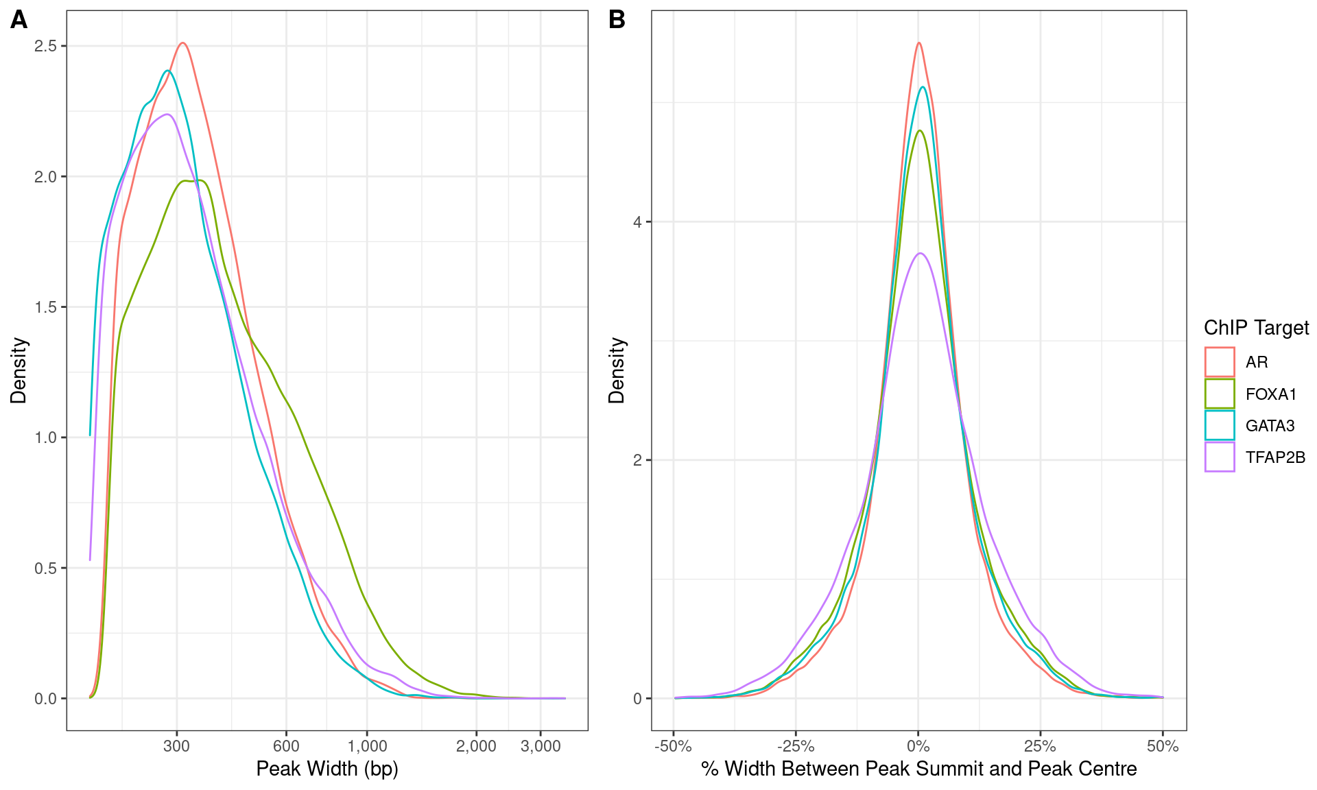
Distributions of A) peak width and B) summit location with peaks.
| Version | Author | Date |
|---|---|---|
| 8836090 | Steve Pederson | 2022-05-26 |
Enrichment of Expected Motifs
Analysis of Motif Enrichment (AME)
grl_by_targets <- dht_consensus %>%
  as_tibble() %>%
  pivot_longer(
    all_of(targets), names_to = "target", values_to = "detected"
  ) %>%
  dplyr::filter(detected) %>%
  group_by(range, H3K27ac) %>%
  summarise(
    targets = paste(sort(target), collapse = " "),
    .groups = "drop"
  ) %>%
  colToRanges(var = "range", seqinfo = sq19) %>%
  sort() %>%
  splitAsList(.$targets)
Union ranges were grouped by the combination of detected AR, FOXA1, GATA3 and TFAP2B binding, then sequences obtained corresponding to each union range.
grl_by_targets %>%
  lapply(
    function(x) {
      tibble(
        `N Sites` = length(x),
        `% H3K27ac` = mean(x$H3K27ac),
        `Median Width` = floor(median(width(x)))
      )
    }
  ) %>%
  bind_rows(.id = "Targets") %>%
  mutate(
    `N Targets` = str_count(Targets, " ") + 1,
    `% H3K27ac` = percent(`% H3K27ac`, 0.1)
  ) %>%
  dplyr::select(contains("Targets"), everything()) %>%
  arrange(`N Targets`, Targets) %>%
  pander(
    justify = "lrrrr",
    caption = "Summary of union ranges and which combinations of the targets were detected."
)| Targets | N Targets | N Sites | % H3K27ac | Median Width |
|---|---|---|---|---|
| AR | 1 | 395 | 13.9% | 241 |
| FOXA1 | 1 | 59,404 | 12.8% | 319 |
| GATA3 | 1 | 4,284 | 19.6% | 234 |
| TFAP2B | 1 | 6,655 | 80.1% | 301 |
| AR FOXA1 | 2 | 3,543 | 17.8% | 505 |
| AR GATA3 | 2 | 158 | 16.5% | 310 |
| AR TFAP2B | 2 | 135 | 55.6% | 414 |
| FOXA1 GATA3 | 2 | 9,760 | 18.1% | 479 |
| FOXA1 TFAP2B | 2 | 3,849 | 64.6% | 513 |
| GATA3 TFAP2B | 2 | 396 | 60.6% | 368 |
| AR FOXA1 GATA3 | 3 | 6,518 | 25.2% | 683 |
| AR FOXA1 TFAP2B | 3 | 1,786 | 62.9% | 639 |
| AR GATA3 TFAP2B | 3 | 61 | 55.7% | 419 |
| FOXA1 GATA3 TFAP2B | 3 | 1,441 | 52.0% | 575 |
| AR FOXA1 GATA3 TFAP2B | 4 | 6,336 | 58.2% | 814 |
meme_db_targets <- meme_db_detected %>%
  dplyr::filter(altname %in% targets) %>%
  to_list()
seq_by_targets <- grl_by_targets %>%
  get_sequence(hg19)
ame_by_targets <- seq_by_targets %>%
  runAme(database = meme_db_targets)
AME from the meme-suite was then run on each sequence to detect the presence of motifs associated with each target within each set of sequences.
ame_by_targets %>%
  bind_rows(.id = "targets") %>%
  mutate(
    motif_id = as.factor(motif_id),
    targets = as.factor(targets),
    TFAP2B = ifelse(
      str_detect(targets, "TFAP2B"), "TFAP2B", "No TFAP2B"
    )
  ) %>%
  dplyr::filter(adj.pvalue < 0.05) %>%
  plot_ame_heatmap(
    id = motif_id,
    value = tp_percent,
    group = targets
  ) +
  geom_label(
    aes(label = percent(tp_percent/100, 0.1)),
    size = 3,
    show.legend = FALSE
  ) +
  facet_grid(TFAP2B ~ motif_alt_id, scales = "free", space = "free") +
  scale_x_discrete(expand = expansion(c(0, 0))) +
  scale_y_discrete(expand = expansion(c(0, 0))) +
  labs(
    x = "Detected Motif",
    y = "Detected Targets",
    fill = expression(widehat("TP%"))
  ) +
  theme(
    axis.text.x = element_text(angle = 0, hjust = 0.5, size = 10),
    axis.text.y = element_text(angle = 0, hjust = 1, size = 10),
    panel.grid = element_blank()
  )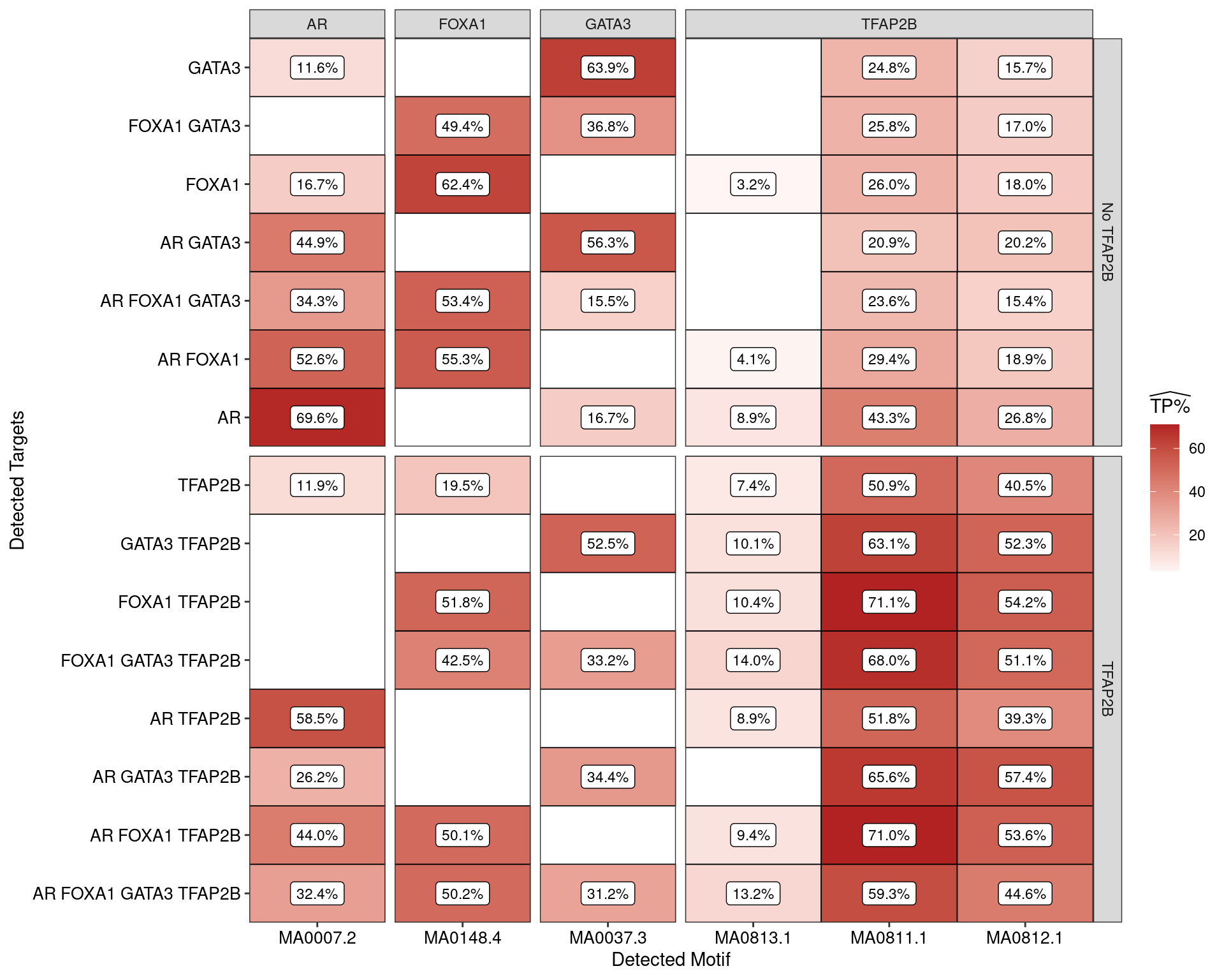
Estimated percentage of true positive matches to all binding motifs associated with each ChIP target. Only values with an enrichment adjusted p-value < 0.05 are shown, such that missing values are able to be confidently assumed as not enriched for the motif. With the possible exception of GATA3 binding in the presence of AR and FOXA1 only, all provide supporting evidence for direct binding of each target to it’s motif
| Version | Author | Date |
|---|---|---|
| 8836090 | Steve Pederson | 2022-05-26 |
Motif Centrality Relative to Each Target
seq_width <- 200
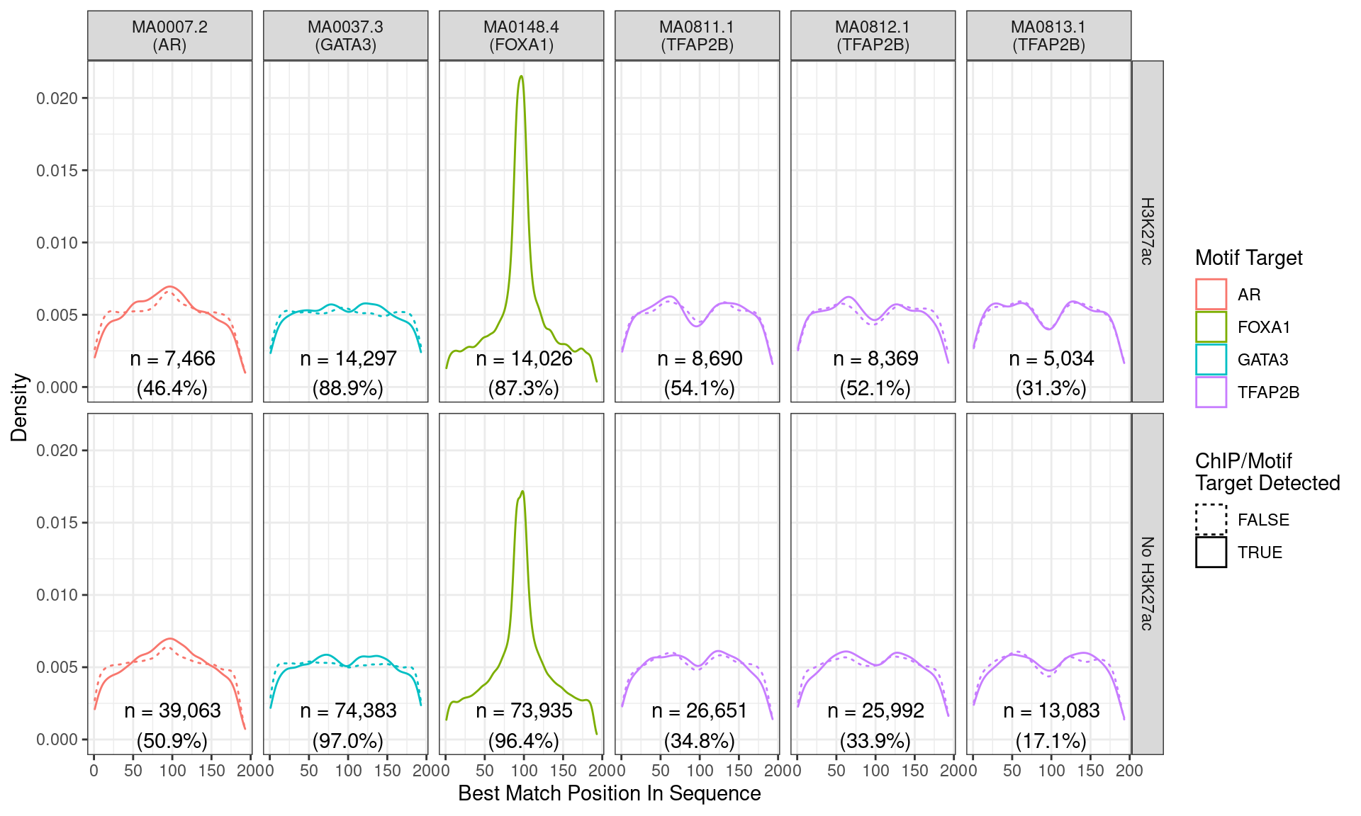
min_score <- percent(0.75, accuracy = 1)In order to assess any association in binding patterns, the binding peak (i.e.) summit of each ChIP target was taken as a viewpoint and the centrality of the best matching sequence motif for that target was assessed. Sequences were extended 200bp from each summit and the best sequence match to each binding motif were retained. Sequence matches with a score > 75% of the highest possible score were initially included before reducing matches to those with the highest score.
The motifs obtained form the larger database were the 6 motifs defined as candidate binding sites for each of the 4 ChIP targets.
meme_info %>%
  dplyr::filter(altname %in% targets) %>%
  arrange(altname, desc(icscore)) %>%
  dplyr::rename(
    `Motif ID` = name,
    Target = altname,
    IC = icscore,
    `Length (bp)` = motif_length
  ) %>%
  pander(
    justify = "llrr",
    caption = paste(
      "Motifs use for checking defined target binding sites. Motifs are ranked",
      "within each ChIP target by information content (IC)."
    )
)| Motif ID | Target | IC | Length (bp) |
|---|---|---|---|
| MA0007.2 | AR | 13.27 | 15 |
| MA0148.4 | FOXA1 | 11.41 | 12 |
| MA0037.3 | GATA3 | 9.749 | 8 |
| MA0813.1 | TFAP2B | 14.31 | 13 |
| MA0812.1 | TFAP2B | 12.56 | 11 |
| MA0811.1 | TFAP2B | 10.86 | 12 |
plot_grid(
  plot_grid(
    plotlist = lapply(
      meme_db_targets %>%
        to_df() %>%
        arrange(altname) %>%
        dplyr::filter(altname != "TFAP2B") %>%
        to_list() %>%
        lapply(
          function(x){
            x@name <- paste0(
              x@name, ": ", x@altname, " (IC = ",
              round(x@icscore, 1), ")"
            )
            x
          }
        ),
      function(x) {
        view_motifs(x) +
          ggtitle(x@name) +
          theme(plot.title = element_text(hjust = 0.5, size = 11))
      }
    ),
    labels = c("A", "B", "C"),
    ncol = 1
  ),
  plot_grid(
    meme_db_targets %>%
      to_df() %>%
      dplyr::filter(altname == "TFAP2B") %>%
      to_list() %>%
      lapply(
          function(x){
            x@name <- paste0(
              x@name, ": ", x@altname, " (IC = ",
              round(x@icscore, 1), ")"
            )
            x
          }
      ) %>%
      view_motifs() +
      theme(plot.title = element_text(hjust = 0.5, size = 9))
  ),
  ncol = 2,
  labels = c("", "D")
)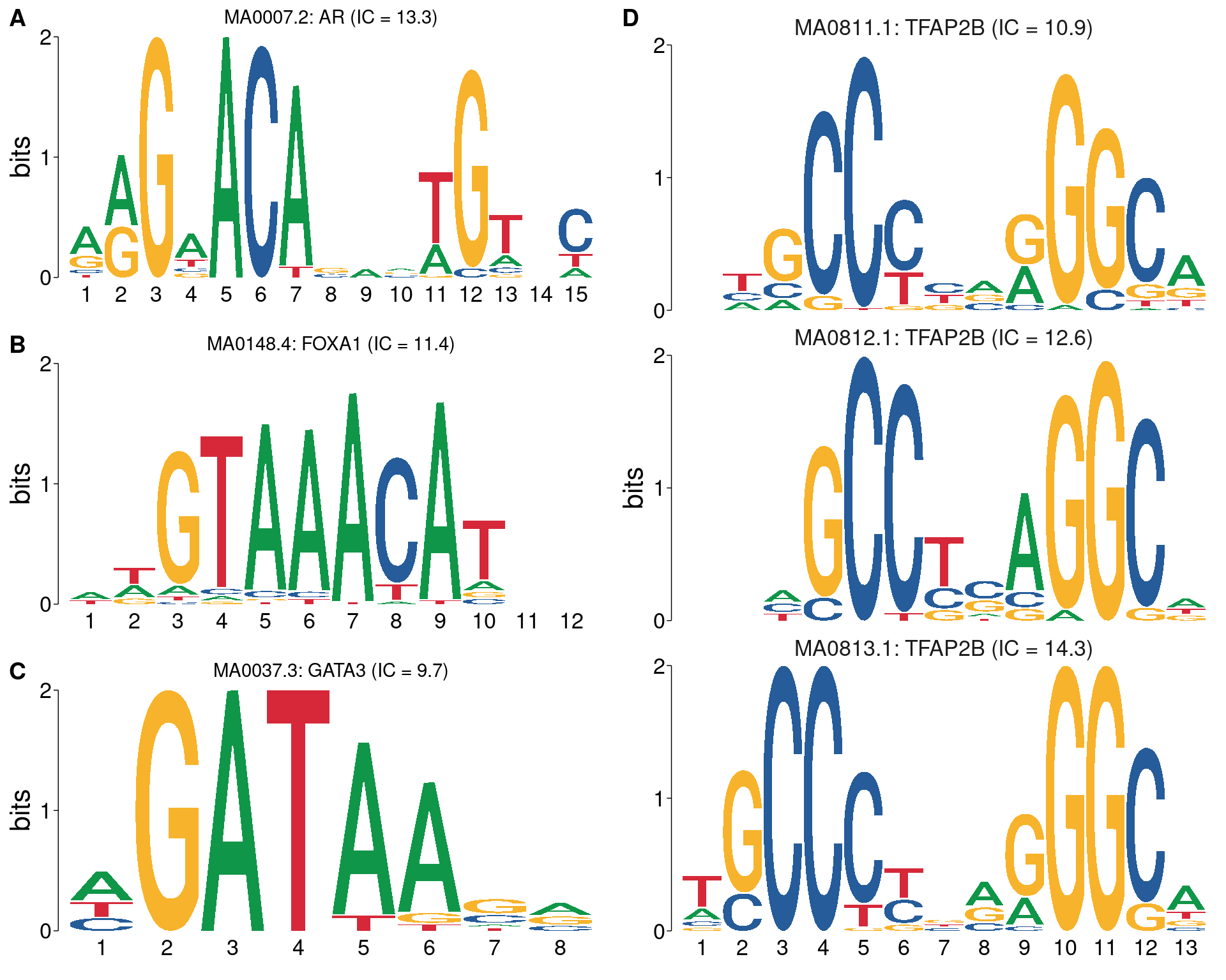
All motifs matching the set of ChIP targets. Motifc in A-C are not aligned with each other, whilst all TFAP2B motifs are shown using the best alignment.
| Version | Author | Date |
|---|---|---|
| 7cfa8e7 | Steve Pederson | 2022-05-26 |
AR
ar_summits <- dht_peaks$AR %>%
  resize(width = 1, fix = 'start') %>%
  shift(shift = .$peak) %>%
  resize(width = seq_width, fix = 'center') %>%
  granges() %>%
  mutate(
    AR = overlapsAny(., subset(dht_consensus, AR)),
    FOXA1 = overlapsAny(., subset(dht_consensus, FOXA1)),
    GATA3 = overlapsAny(., subset(dht_consensus, GATA3)),
    TFAP2B = overlapsAny(., subset(dht_consensus, TFAP2B)),
    H3K27ac = overlapsAny(., features)
  )
seq_ar_summits <- ar_summits %>%
  get_sequence(hg19)
views_ar_summits <- as(seq_ar_summits, "Views") %>%
  setNames(names(seq_ar_summits))
matches_ar_summits <-meme_db_targets %>%
  lapply(
    getBestMatch,
    subject = views_ar_summits,
    min.score = min_score
  ) %>%
  setNames(
    vapply(meme_db_targets, function(x) x@name, character(1))
  ) %>%
  bind_rows(.id = "name") %>%
  left_join(
    dplyr::select(meme_info, name, altname, motif_length),
    by = "name"
  ) %>%
    dplyr::rename(range = view_name) %>%
  left_join(as_tibble(ar_summits), by = "range" ) %>%
  arrange(view) %>%
  mutate(
    target_detected = case_when(
      altname == "AR" ~ AR,
      altname == "FOXA1" ~ FOXA1,
      altname == "GATA3" ~ GATA3,
      altname == "TFAP2B" ~ TFAP2B
    )
  ) %>%
  dplyr::select(
    range,
    any_of(targets), H3K27ac,
    name, altname, target_detected,
    pos = start_in_view, width, strand, seq
  )
matches_ar_summits %>%
mutate(
label = glue("{name}\n({altname})"),
H3K27ac = ifelse(H3K27ac, "H3K27ac", "No H3K27ac")
) %>%
ggplot(aes(pos, stat(density), colour = altname)) +
geom_density(aes(linetype = target_detected)) +
geom_text(
aes(x = seq_width/2, y = 0.001, label = lab),
data = . %>%
group_by(label, H3K27ac) %>%
summarise(
n = dplyr::n(), .groups = "drop"
) %>%
mutate(
lab = case_when(
H3K27ac == "H3K27ac" ~ glue(
"n = {comma(n)}\n({percent(n/sum(ar_summits$H3K27ac), 0.1)})"
),
H3K27ac == "No H3K27ac" ~ glue(
"n = {comma(n)}\n({percent(n/sum(!ar_summits$H3K27ac), 0.1)})"
)
)
),
colour = "black",
inherit.aes = FALSE
) +
facet_grid(H3K27ac ~ label) +
scale_linetype_manual(values = c(3, 1)) +
labs(
x = "Best Match Position In Sequence",
y = "Density",
colour = "Motif Target",
linetype = "Target Detected"
)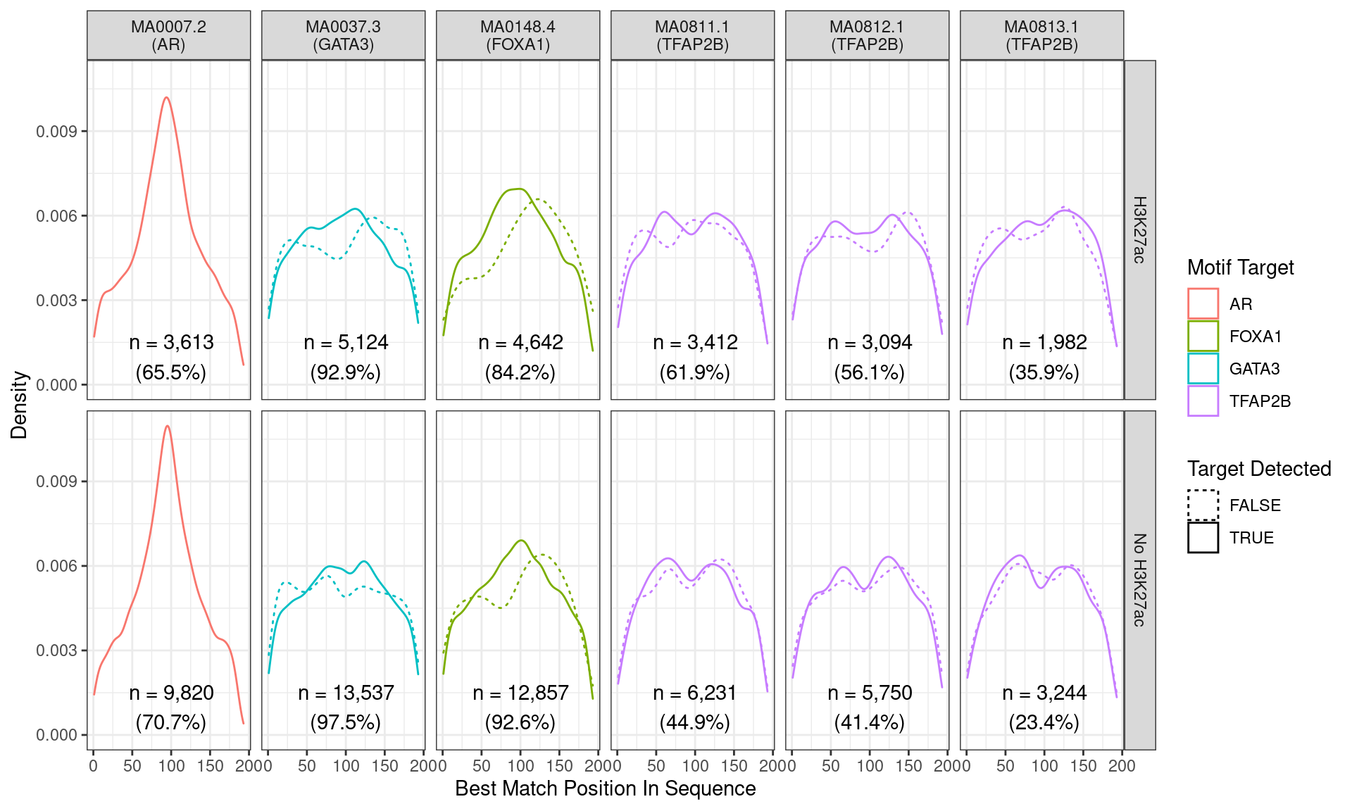
Position of the best match for each motif using sequences centred at the summits of AR binding sites. Sites where the ChIP target was not detected are shown as dashed lines, and panels are separated by H3K27ac status. No visual difference in AR motif centrality was detected due to H3K27ac signal. A slight tendency for the best FOXA1 to also appear centrally was noted.
Across all motifs which were considered to represent possible matches to the binding site of AR, matches to one or more of the motifs were found in 13,433 (69.2%) of the 19,406 queried sequences.
FOXA1
foxa1_summits <- dht_peaks$FOXA1 %>%
  resize(width = 1, fix = 'start') %>%
  shift(shift = .$peak) %>%
  resize(width = seq_width, fix = 'center') %>%
  granges() %>%
  mutate(
    AR = overlapsAny(., subset(dht_consensus, AR)),
    FOXA1 = overlapsAny(., subset(dht_consensus, FOXA1)),
    GATA3 = overlapsAny(., subset(dht_consensus, GATA3)),
    TFAP2B = overlapsAny(., subset(dht_consensus, TFAP2B)),
    H3K27ac = overlapsAny(., features)
  )
seq_foxa1_summits <- foxa1_summits %>%
  get_sequence(hg19)
views_foxa1_summits <- as(seq_foxa1_summits, "Views") %>%
  setNames(names(seq_foxa1_summits))
matches_foxa1_summits <- meme_db_targets %>%
  lapply(
    getBestMatch,
    subject = views_foxa1_summits,
    min.score = min_score
  ) %>%
  setNames(
    vapply(meme_db_targets, function(x) x@name, character(1))
  ) %>%
  bind_rows(.id = "name") %>%
  left_join(
    dplyr::select(meme_info, name, altname, motif_length),
    by = "name"
  ) %>%
    dplyr::rename(range = view_name) %>%
  left_join(as_tibble(foxa1_summits), by = "range" ) %>%
  arrange(view) %>%
  mutate(
    target_detected = case_when(
      altname == "AR" ~ AR,
      altname == "FOXA1" ~ FOXA1,
      altname == "GATA3" ~ GATA3,
      altname == "TFAP2B" ~ TFAP2B
    )
  ) %>%
  dplyr::select(
    range,
    any_of(targets), H3K27ac,
    name, altname, target_detected,
    pos = start_in_view, width, strand, seq
  )
matches_foxa1_summits %>%
mutate(
label = glue("{name}\n({altname})"),
H3K27ac = ifelse(H3K27ac, "H3K27ac", "No H3K27ac")
) %>%
ggplot(aes(pos, stat(density), colour = altname)) +
geom_density(aes(linetype = target_detected)) +
geom_text(
aes(x = seq_width/2, y = 0.001, label = lab),
data = . %>%
group_by(label, H3K27ac) %>%
summarise(
n = dplyr::n(), .groups = "drop"
) %>%
mutate(
lab = case_when(
H3K27ac == "H3K27ac" ~ glue(
"n = {comma(n)}\n({percent(n/sum(foxa1_summits$H3K27ac), 0.1)})"
),
H3K27ac == "No H3K27ac" ~ glue(
"n = {comma(n)}\n({percent(n/sum(!foxa1_summits$H3K27ac), 0.1)})"
)
)
),
colour = "black",
inherit.aes = FALSE
) +
facet_grid(H3K27ac ~ label) +
scale_linetype_manual(values = c(3, 1)) +
labs(
x = "Best Match Position In Sequence",
y = "Density",
colour = "Motif Target",
linetype = "ChIP/Motif\nTarget Detected"
)
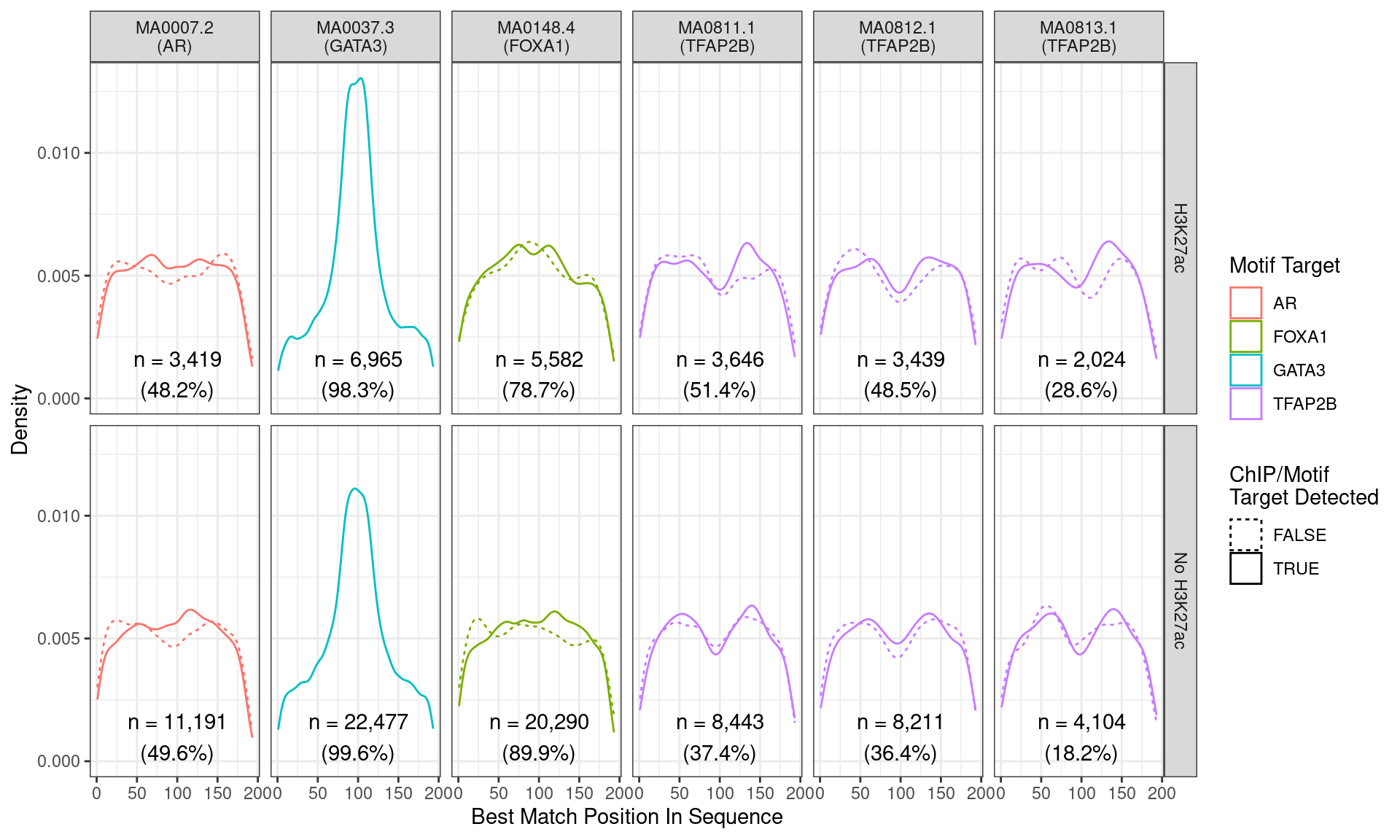
Position of the best match for each motif using sequences centred at the summits of FOXA1 binding sites. Sites where the ChIP target was not detected are shown as dashed lines, and panels are separated by H3K27ac status. No visual difference in FOXA1 motif centrality was detected due to H3K27ac signal. A slight tendency for the best FOXA1 to also appear centrally was noted.
Across all motifs which were considered to represent possible matches to the binding site of FOXA1, matches to one or more of the motifs were found in 87,961 (94.8%) of the 92,751 queried sequences.
GATA3
gata3_summits <- dht_peaks$GATA3 %>%
  resize(width = 1, fix = 'start') %>%
  shift(shift = .$peak) %>%
  resize(width = seq_width, fix = 'center') %>%
  granges() %>%
  mutate(
    AR = overlapsAny(., subset(dht_consensus, AR)),
    FOXA1 = overlapsAny(., subset(dht_consensus, FOXA1)),
    GATA3 = overlapsAny(., subset(dht_consensus, GATA3)),
    TFAP2B = overlapsAny(., subset(dht_consensus, TFAP2B)),
    H3K27ac = overlapsAny(., features)
  )
seq_gata3_summits <- gata3_summits %>%
  get_sequence(hg19)
views_gata3_summits <- as(seq_gata3_summits, "Views") %>%
  setNames(names(seq_gata3_summits))
matches_gata3_summits <- meme_db_targets %>%
  lapply(
    getBestMatch,
    subject = views_gata3_summits,
    min.score = min_score
  ) %>%
  setNames(
    vapply(meme_db_targets, function(x) x@name, character(1))
  ) %>%
  bind_rows(.id = "name") %>%
  left_join(
    dplyr::select(meme_info, name, altname, motif_length),
    by = "name"
  ) %>%
    dplyr::rename(range = view_name) %>%
  left_join(as_tibble(gata3_summits), by = "range" ) %>%
  arrange(view) %>%
  mutate(
    target_detected = case_when(
      altname == "AR" ~ AR,
      altname == "FOXA1" ~ FOXA1,
      altname == "GATA3" ~ GATA3,
      altname == "TFAP2B" ~ TFAP2B
    )
  ) %>%
  dplyr::select(
    range,
    any_of(targets), H3K27ac,
    name, altname, target_detected,
    pos = start_in_view, width, strand, seq
  )
matches_gata3_summits %>%
mutate(
label = glue("{name}\n({altname})"),
H3K27ac = ifelse(H3K27ac, "H3K27ac", "No H3K27ac")
) %>%
ggplot(aes(pos, stat(density), colour = altname)) +
geom_density(aes(linetype = target_detected)) +
geom_text(
aes(x = seq_width/2, y = 0.001, label = lab),
data = . %>%
group_by(label, H3K27ac) %>%
summarise(
n = dplyr::n(), .groups = "drop"
) %>%
mutate(
lab = case_when(
H3K27ac == "H3K27ac" ~ glue(
"n = {comma(n)}\n({percent(n/sum(gata3_summits$H3K27ac), 0.1)})"
),
H3K27ac == "No H3K27ac" ~ glue(
"n = {comma(n)}\n({percent(n/sum(!gata3_summits$H3K27ac), 0.1)})"
)
)
),
colour = "black",
inherit.aes = FALSE
) +
facet_grid(H3K27ac ~ label) +
scale_linetype_manual(values = c(3, 1)) +
labs(
x = "Best Match Position In Sequence",
y = "Density",
colour = "Motif Target",
linetype = "ChIP/Motif\nTarget Detected"
)
Position of the best match for each motif using sequences centred at the summits of GATA3 binding sites. Sites where the ChIP target was not detected are shown as dashed lines, and panels are separated by H3K27ac status. No visual difference in GATA3 motif centrality was detected due to H3K27ac signal. A slight tendency for the best FOXA1 to also appear centrally was noted.
Across all motifs which were considered to represent possible matches to the binding site of GATA3, matches to one or more of the motifs were found in 29,442 (99.2%) of the 29,666 queried sequences.
TFAP2B
tfap2b_summits <- dht_peaks$TFAP2B %>%
  resize(width = 1, fix = 'start') %>%
  shift(shift = .$peak) %>%
  resize(width = seq_width, fix = 'center') %>%
  granges() %>%
  mutate(
    AR = overlapsAny(., subset(dht_consensus, AR)),
    FOXA1 = overlapsAny(., subset(dht_consensus, FOXA1)),
    GATA3 = overlapsAny(., subset(dht_consensus, GATA3)),
    TFAP2B = overlapsAny(., subset(dht_consensus, TFAP2B)),
    H3K27ac = overlapsAny(., features)
  )
seq_tfap2b_summits <- tfap2b_summits %>%
  get_sequence(hg19)
views_tfap2b_summits <- as(seq_tfap2b_summits, "Views") %>%
  setNames(names(seq_tfap2b_summits))
matches_tfap2b_summits <- meme_db_targets %>%
  lapply(
    getBestMatch,
    subject = views_tfap2b_summits,
    min.score = min_score
  ) %>%
  setNames(
    vapply(meme_db_targets, function(x) x@name, character(1))
  ) %>%
  bind_rows(.id = "name") %>%
  left_join(
    dplyr::select(meme_info, name, altname, motif_length),
    by = "name"
  ) %>%
    dplyr::rename(range = view_name) %>%
  left_join(as_tibble(tfap2b_summits), by = "range" ) %>%
  arrange(view) %>%
  mutate(
    target_detected = case_when(
      altname == "AR" ~ AR,
      altname == "FOXA1" ~ FOXA1,
      altname == "GATA3" ~ GATA3,
      altname == "TFAP2B" ~ TFAP2B
    )
  ) %>%
  dplyr::select(
    range,
    any_of(targets), H3K27ac,
    name, altname, target_detected,
    pos = start_in_view, width, strand, seq
  )
matches_tfap2b_summits %>%
mutate(
label = glue("{name}\n({altname})"),
H3K27ac = ifelse(H3K27ac, "H3K27ac", "No H3K27ac")
) %>%
ggplot(aes(pos, stat(density), colour = altname)) +
geom_density(aes(linetype = target_detected)) +
geom_text(
aes(x = seq_width/2, y = 0.001, label = lab),
data = . %>%
group_by(label, H3K27ac) %>%
summarise(
n = dplyr::n(), .groups = "drop"
) %>%
mutate(
lab = case_when(
H3K27ac == "H3K27ac" ~ glue(
"n = {comma(n)}\n({percent(n/sum(tfap2b_summits$H3K27ac), 0.1)})"
),
H3K27ac == "No H3K27ac" ~ glue(
"n = {comma(n)}\n({percent(n/sum(!tfap2b_summits$H3K27ac), 0.1)})"
)
)
),
colour = "black",
inherit.aes = FALSE
) +
facet_grid(H3K27ac ~ label) +
scale_linetype_manual(values = c(3, 1)) +
labs(
x = "Best Match Position In Sequence",
y = "Density",
colour = "Motif Target",
linetype = "ChIP/Motif\nTarget Detected"
)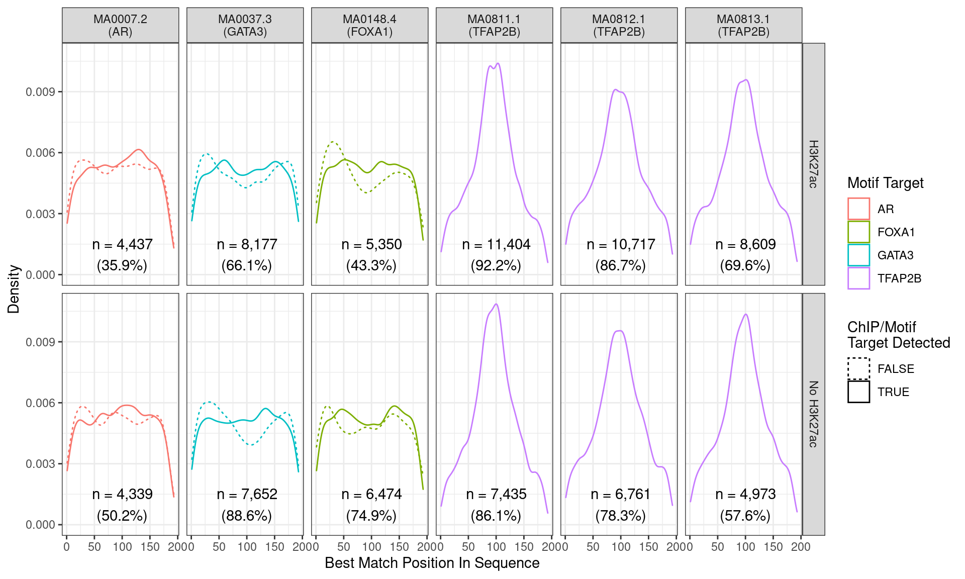
Position of the best match for each motif using sequences centred at the summits of TFAP2B binding sites. Sites where the ChIP target was not detected are shown as dashed lines, and panels are separated by H3K27ac status. No visual difference in TFAP2B motif centrality was detected. All other motifs appeared to be uniformly distributed amongst the sequences.
Across all motifs which were considered to represent possible matches to the binding site of TFAP2\(\beta\), matches to one or more of the motifs were found in 20,375 (97.0%) of the 21,008 queried sequences.
Distance Between Motifs
Whilst the above section revealed some degree of association between AR and FOXA1 sites, as well as clear separation between all targets and TFAP2B motifs, the distribution of distances between motif matches can also be addressed directly.
AR
matches_ar_summits %>%
  group_by(range) %>%
  dplyr::filter(any(altname == "AR")) %>%
  mutate(
    ar_pos = pos[altname == "AR"],
    ar_strand = strand[altname == "AR"]
  ) %>%
  ungroup() %>%
  mutate(
    ar_motif_dist = abs(pos - ar_pos),
    label = glue("{name} ({altname})"),
    H3K27ac = ifelse(H3K27ac, "H3K27ac", "No H3K27ac"),
    target_detected = ifelse(target_detected, "Target Detected", "Target Undetected")
  ) %>%
  dplyr::filter(altname != "AR") %>%
  group_by(name, target_detected, H3K27ac) %>%
  mutate(
    q = rank(ar_motif_dist, ties = "first") / length(ar_motif_dist)
  ) %>%
  dplyr::filter(q <= 0.5) %>%
  ggplot(
    aes(ar_motif_dist, q, colour = label)
  ) +
  geom_line() +
  facet_grid(H3K27ac ~ target_detected) +
  scale_y_continuous(labels= percent) +
  labs(
    x = "Distance from AR motif",
    y = "Percentile",
    colour = "Motif Target",
    linetype = "ChIP/Motif\nTarget Detected"
  )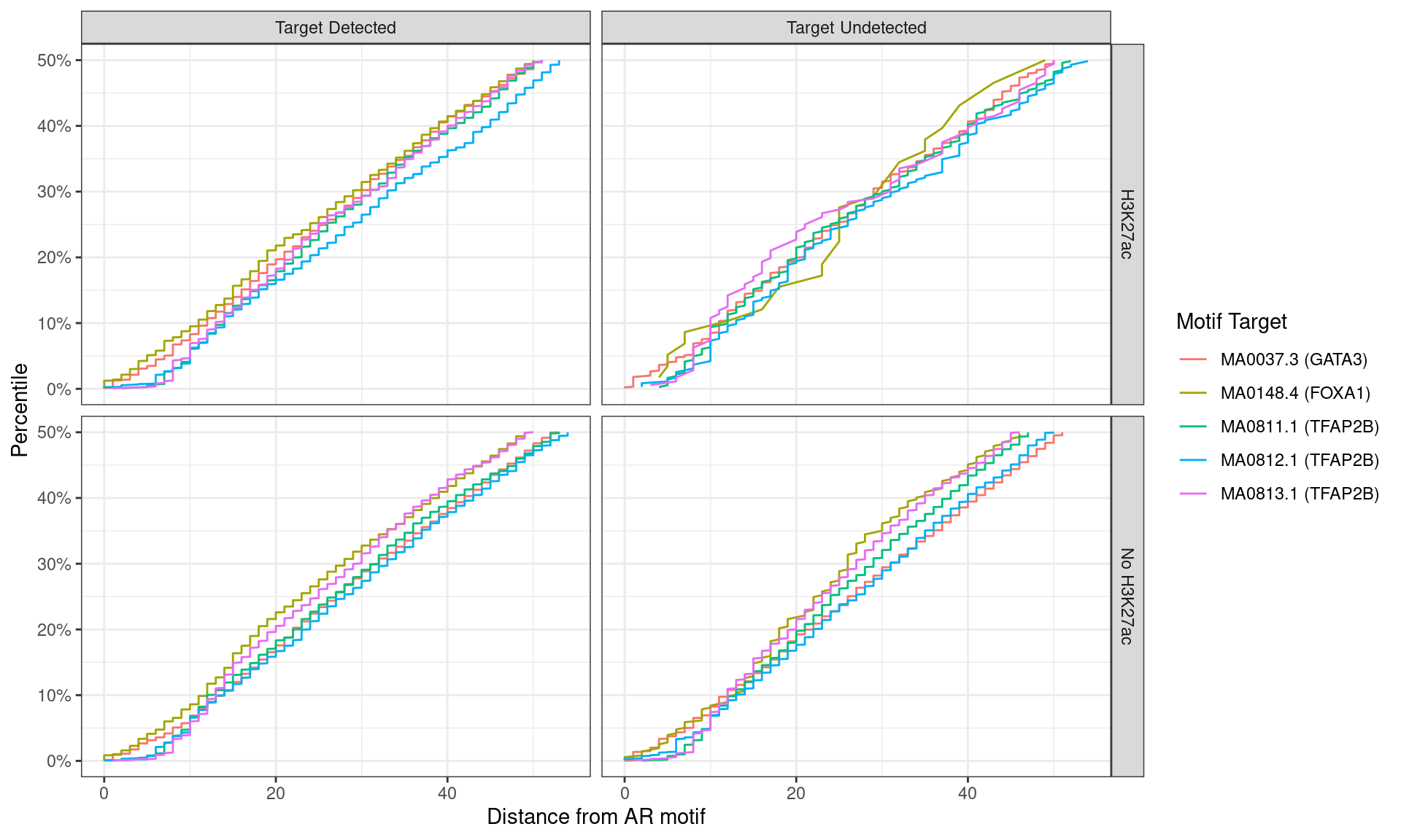
Distance between best matching motif and the best matching AR motif, showing data to the 50th percentile of distances. No noticable difference was noticed between individual motifs, H3K27ac status, or whether the ChIP target was detected within the AR peak.
| Version | Author | Date |
|---|---|---|
| 1bf46f7 | Steve Pederson | 2022-05-27 |
FOXA1
matches_foxa1_summits %>%
  group_by(range) %>%
  dplyr::filter(any(altname == "FOXA1")) %>%
  mutate(
    foxa1_pos = pos[altname == "FOXA1"],
    foxa1_strand = strand[altname == "FOXA1"]
  ) %>%
  ungroup() %>%
  mutate(
    foxa1_motif_dist = abs(pos - foxa1_pos),
    label = glue("{name} ({altname})"),
    H3K27ac = ifelse(H3K27ac, "H3K27ac", "No H3K27ac"),
    target_detected = ifelse(target_detected, "Target Detected", "Target Undetected")
  ) %>%
  dplyr::filter(altname != "FOXA1") %>%
  group_by(name, target_detected, H3K27ac) %>%
  mutate(
    q = rank(foxa1_motif_dist, ties = "first") / length(foxa1_motif_dist)
  ) %>%
  dplyr::filter(q <= 0.5) %>%
  ggplot(
    aes(foxa1_motif_dist, q, colour = label)
  ) +
  geom_line() +
  facet_grid(H3K27ac ~ target_detected) +
  scale_y_continuous(labels= percent) +
  labs(
    x = "Distance from FOXA1 motif",
    y = "Percentile",
    colour = "Motif Target",
    linetype = "ChIP/Motif\nTarget Detected"
  )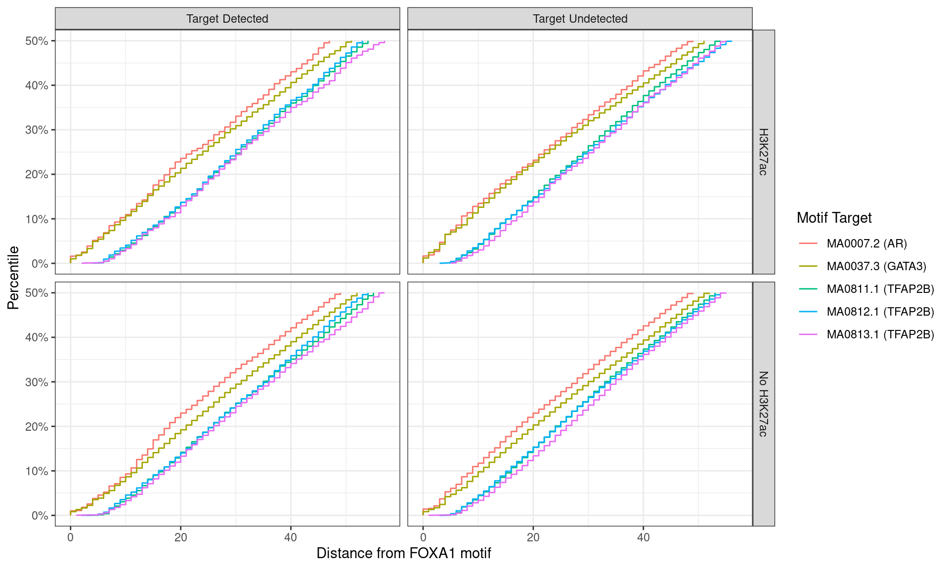
Distance between best matching motif and the best matching FOXA1 motif, showing data to the 50th percentile of distances. No noticable difference was noticed between individual motifs, H3K27ac status, or whether the ChIP target was detected within the FOXA1 peak.
| Version | Author | Date |
|---|---|---|
| 1bf46f7 | Steve Pederson | 2022-05-27 |
GATA3
matches_gata3_summits %>%
  group_by(range) %>%
  dplyr::filter(any(altname == "GATA3")) %>%
  mutate(
    gata3_pos = pos[altname == "GATA3"],
    gata3_strand = strand[altname == "GATA3"]
  ) %>%
  ungroup() %>%
  mutate(
    gata3_motif_dist = abs(pos - gata3_pos),
    label = glue("{name} ({altname})"),
    H3K27ac = ifelse(H3K27ac, "H3K27ac", "No H3K27ac"),
    target_detected = ifelse(target_detected, "Target Detected", "Target Undetected")
  ) %>%
  dplyr::filter(altname != "GATA3") %>%
  group_by(name, target_detected, H3K27ac) %>%
  mutate(
    q = rank(gata3_motif_dist, ties = "first") / length(gata3_motif_dist)
  ) %>%
  dplyr::filter(q <= 0.5) %>%
  ggplot(
    aes(gata3_motif_dist, q, colour = label)
  ) +
  geom_line() +
  facet_grid(H3K27ac ~ target_detected) +
  scale_y_continuous(labels= percent) +
  scale_linetype_manual(values = c(3, 1)) +
  labs(
    x = "Distance from GATA3 motif",
    y = "Percentile",
    colour = "Motif Target",
    linetype = "ChIP/Motif\nTarget Detected"
  )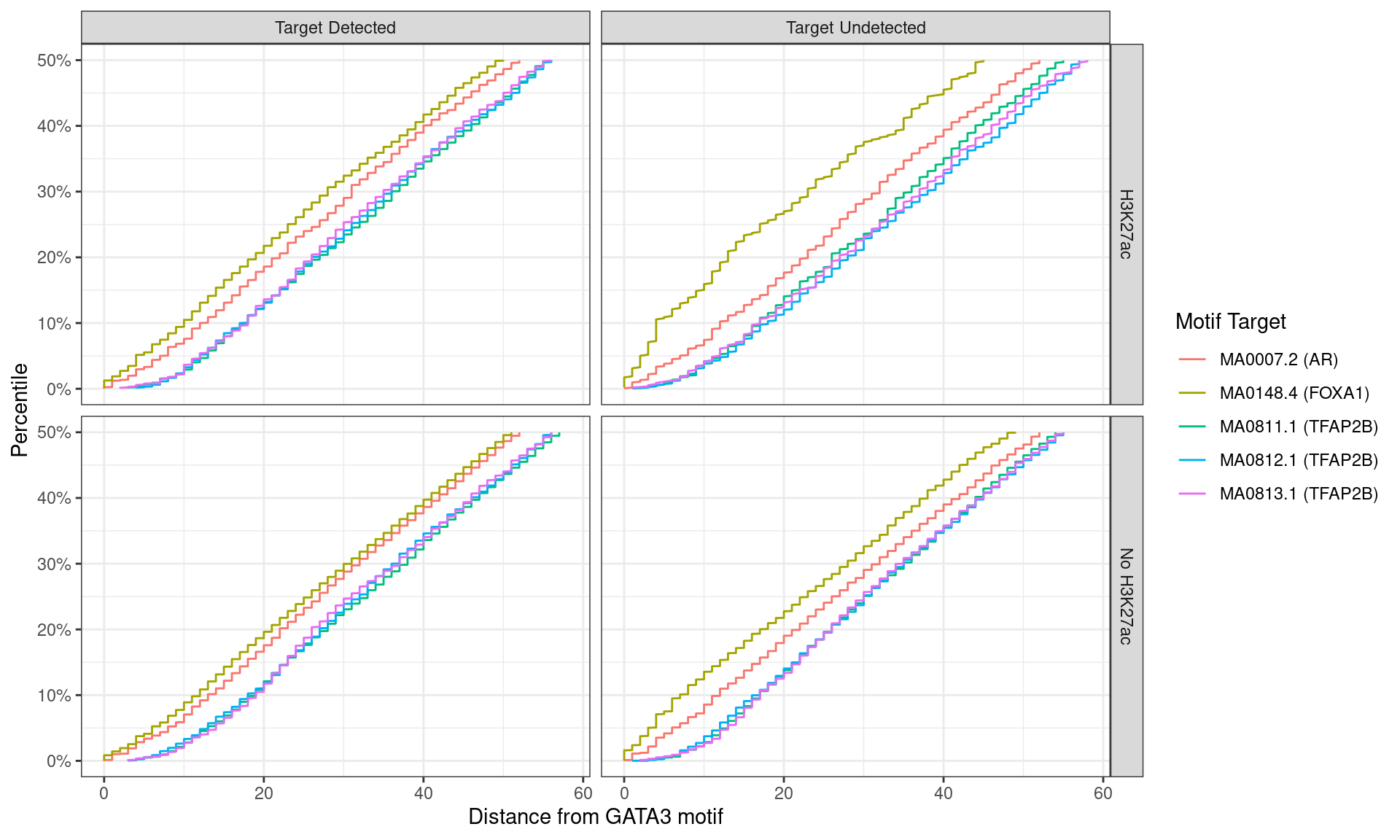
Distance between best matching motif and the best matching GATA3 motif, showing data to the 50th percentile of distances. FOXA1 motifs tended to be further from the GATA3 motif for peaks where FOXA1 was detected.
| Version | Author | Date |
|---|---|---|
| 1bf46f7 | Steve Pederson | 2022-05-27 |
TFAP2B
matches_tfap2b_summits %>%
  group_by(range) %>%
  dplyr::filter(any(altname == "TFAP2B")) %>%
  mutate(
    tfap2b_pos = pos[altname == "TFAP2B"][1],
  ) %>%
  ungroup() %>%
  mutate(
    tfap2b_motif_dist = abs(pos - tfap2b_pos),
    label = glue("{name} ({altname})"),
    H3K27ac = ifelse(H3K27ac, "H3K27ac", "No H3K27ac"),
    target_detected = ifelse(target_detected, "Target Detected", "Target Undetected")
  ) %>%
  dplyr::filter(altname != "TFAP2B") %>%
  group_by(name, target_detected, H3K27ac) %>%
  mutate(
    q = rank(tfap2b_motif_dist, ties = "first") / length(tfap2b_motif_dist)
  ) %>%
  dplyr::filter(q <= 0.5) %>%
  ggplot(
    aes(tfap2b_motif_dist, q, colour = label)
  ) +
  geom_line() +
  facet_grid(H3K27ac ~ target_detected) +
  scale_y_continuous(labels= percent) +
  scale_linetype_manual(values = c(3, 1)) +
  labs(
    x = "Distance from TFAP2B motif",
    y = "Percentile",
    colour = "Motif Target",
    linetype = "ChIP/Motif\nTarget Detected"
  )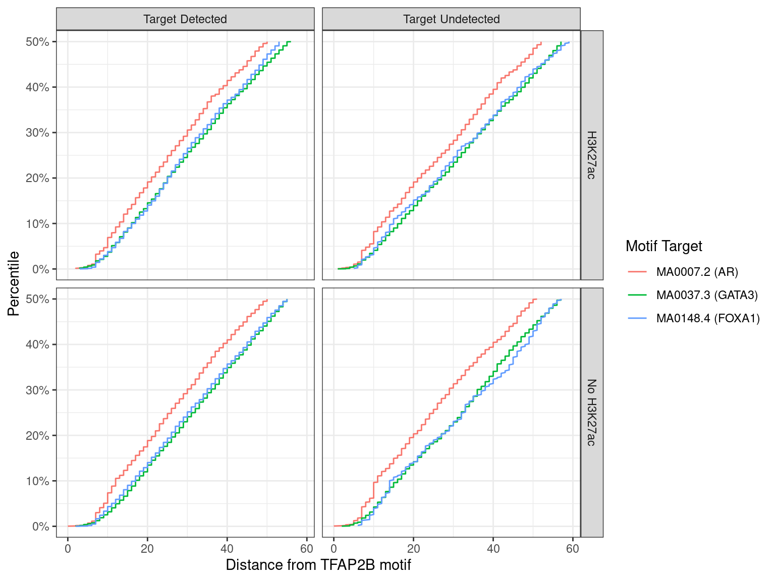
Distance between best matching motif and the best matching TFAP2B motif, showing data to the 50th percentile of distances. No noticable difference was noticed between individual motifs, H3K27ac status, or whether the ChIP target was detected within the TFAP2B peak.
| Version | Author | Date |
|---|---|---|
| 1bf46f7 | Steve Pederson | 2022-05-27 |
Motif Discovery
The above steps essentially perform checks on the data and verify that the expected binding motifs are generally driving binding of each target. A further step would be to determine any enriched binding motifs within the union peaks which are able to be confidently assigned to putative co-factors. For this section, key comparisons were chosen as this enables detection of cofactors which may be driving key binding patterns. Novel sequence motifs were first defined using STREME, which uses a suffix tree based approach to determining enrichment of sequence motifs.
All 4 Targets Bound: H3K27ac Vs No H3K27ac
A comparison between binding sites where all 4 targets were found was performed based on this showing regulatory activity (overlap with H3K27ac-derived features) and no regulatory activity (i.e. no H3K27ac overlap).
seq_all4_by_h3k27ac <- dht_consensus %>%
  filter(!!!syms(targets)) %>%
  split(.$H3K27ac) %>%
  setNames(c("no_h3k27ac", "h3k27ac")) %>%
  get_sequence(hg19) %>%
  as.list()
streme_all4_by_h3k27ac_rds <- here::here(
  "output", "streme", "all4_by_h3k27ac.rds"
)
if (!dir.exists(dirname(streme_all4_by_h3k27ac_rds))) dir.create(
  dirname(streme_all4_by_h3k27ac_rds)
)
if (!file.exists(streme_all4_by_h3k27ac_rds)) {
  streme_all4_by_h3k27ac <- runStreme(
    input = seq_all4_by_h3k27ac$h3k27ac,
    control = seq_all4_by_h3k27ac$no_h3k27ac,
    thresh = 0.01
  ) %>%
    as_tibble() %>%
    mutate(
      eval = case_when(
        is.na(eval) ~ pval * nrow(.),
        !is.na(eval) ~ eval
      )
    )
  write_rds(
    x = streme_all4_by_h3k27ac,
    file = streme_all4_by_h3k27ac_rds
  )
} else {
  streme_all4_by_h3k27ac <- read_rds(streme_all4_by_h3k27ac_rds)
}
tomtom_all4_by_h3k27ac <- streme_all4_by_h3k27ac %>%
  to_list() %>%
  runTomTom(
    database = to_list(meme_db_detected),
    thresh = 0.1
  )
streme_to_keep_all4_by_h3k27ac <- tomtom_all4_by_h3k27ac %>%
  lapply(function(x) x$best_match_name) %>%
  vapply(length, integer(1)) %>%
  is_greater_than(0)
Using the default setting of STREME, 40 candidate sequence motifs were detected. TomTom was subsequently used to match candidate motifs with those in the database of detected sequences. To ensure only high-quality candidates were retained, matches with a p-value > 0.1 for similarity were discarded. This strategy gave 7 candidate motifs able to be matched to the database and retained as high-quality motifs.
pl <- tomtom_all4_by_h3k27ac[streme_to_keep_all4_by_h3k27ac] %>%
  bind_rows() %>%
  arrange(desc(nsites)) %>%
  to_list() %>%
  lapply(
    function(x) {
      nm <- paste0(
        x@altname,
        " (IC: ", round(x@icscore, 1), "; n = ", x@nsites, ")\n",
        x@extrainfo[["best_match_altname"]]
      )
      view_motifs(x) +
        ggtitle(nm) +
        theme(
          plot.title = element_text(hjust = 0.5, size = 8),
          axis.text = element_text(size = 8),
          axis.title = element_text(size = 8)
        )
    }
  )
plot_grid(plotlist = pl)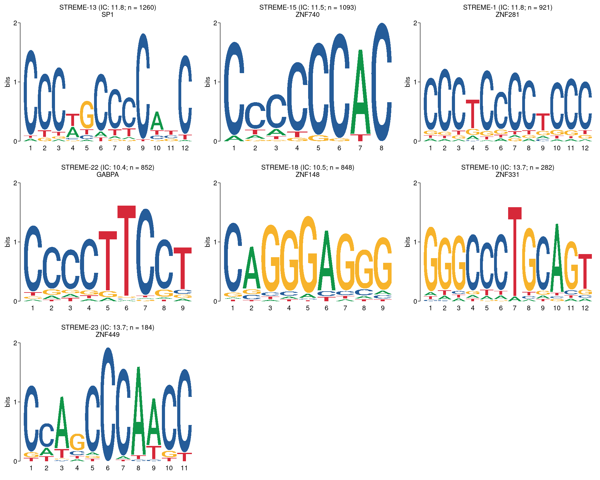
All motifs detected by STREME using a threshold of \(p \leq 0.01\) and with high-quality matches to the database of motifs. The name of the best matching motif is given as the second line of the title, although this may not be the true TF which binds to the motif. Motifs are ordered by the number of times they appear in the sequences, noting the motifs with high information content tend to lead to fewer hits.
| Version | Author | Date |
|---|---|---|
| 7cfa8e7 | Steve Pederson | 2022-05-26 |
tomtom_all4_by_h3k27ac[streme_to_keep_all4_by_h3k27ac] %>%
  lapply(
    function(x) {
      tt <- x$tomtom[[1]]
      mt <- lapply(
        tt$match_motif,
        function(um) {
          nm <- paste0(um@name, " (", um@altname, ")")
          um@name <- nm
          um
        }
      )
      x$tomtom[[1]]$match_motif <- mt
      x
    }
  ) %>%
  lapply(
    function(x) {
      mutate(x, tomtom_logos = view_tomtom_hits(x))
    }
  ) %>%
  bind_rows() %>%
  dplyr::select(
    motif, id = altname, IC = icscore, nsites,
    best_match_name, best_match_altname, best_match_motif,
    tomtom_logos, tomtom, pval , eval
  ) %>%
  mutate(
    tomtom_logos = tomtom_logos %>%
      lapply(
        function(x) {
          n <- length(levels(x$data$motif.id))
          ggplot_image(x, height = px(60 + n*60), aspect_ratio = 180 / (100 + n*30))
        }
      ),
    `All Matches` = vapply(
      tomtom,
      function(x) {
        paste(x$match_altname, collapse = ", ")
      },
      character(1)
    )
  ) %>%
  dplyr::select(
    `STREME ID` = id, `Best Match` = best_match_altname, `All Matches`,
    IC, `Matches Found` = nsites, `P-value` = pval, `E-value` = eval,
    `TOMTOM Matches` = tomtom_logos
  ) %>%
  gt(
    caption = paste(
      "All STREME-detected motifs with putative matches in the motif database.",
      "The motif database was restricted to motifs associated with detected genes.",
      "The information content (IC) is given along with the number of sequences",
      "the motif was found in. The E-value is equivalent to an adjusted p-value",
      "for the likelihood of the detected motif being non-artefactual."
    ),
    id = "tomtom"
  ) %>%
  fmt_markdown(contains("TOMTOM")) %>%
  fmt_number(contains("val"), decimals = 4) %>%
  fmt_number("Matches Found", decimals = 0, use_seps = TRUE) %>%
  fmt_number("IC", decimals = 2) %>%
  tab_spanner(
    label = "Database Matches",
    columns = all_of(c("Best Match", "All Matches"))
  ) %>%
  tab_spanner(
    label = "Statistics",
    columns = c("IC", "Matches Found", "P-value", "E-value")
  ) %>%
  text_transform(
    locations = cells_body(columns = "All Matches"),
    fn = function(x) str_replace_all(x, ", ", "<br>")
  ) %>%
  tab_options(
    table.width = pct(100),
    table.font.size = px(12)
  ) %>%
  opt_css(
    css = "
    #tomtom .gt_row{
      vertical-align: top
    }
    "
)| STREME ID | Database Matches | Statistics | TOMTOM Matches | ||||
|---|---|---|---|---|---|---|---|
| Best Match | All Matches | IC | Matches Found | P-value | E-value | ||
| STREME-1 | ZNF281 | ZNF281 ZNF148 |
11.84 | 921 | 0.0001 | 0.0024 | 
|
| STREME-10 | ZNF331 | ZNF331 | 13.75 | 282 | 0.0035 | 0.0840 | 
|
| STREME-13 | SP1 | SP1 SP2 KLF10 KLF12 |
11.79 | 1,260 | 0.0044 | 0.1056 | 
|
| STREME-15 | ZNF740 | ZNF740 KLF4 |
11.50 | 1,093 | 0.0071 | 0.1704 | 
|
| STREME-18 | ZNF148 | ZNF148 | 10.48 | 848 | 0.0088 | 0.2112 | 
|
| STREME-22 | GABPA | GABPA ELF3 ELF1 |
10.43 | 852 | 0.0680 | 1.6320 | 
|
| STREME-23 | ZNF449 | ZNF449 | 13.75 | 184 | 0.0870 | 2.0880 | 
|
Novel Motif Centrality
Using the same approach as before, i.e. looking the lens of each ChIP target’s binding peak, any proximity effect with each ChIP target was assessed.
AR
streme_ar_summits <- streme_all4_by_h3k27ac %>%
  dplyr::slice(which(streme_to_keep_all4_by_h3k27ac)) %>%
  to_list %>%
  lapply(
    getBestMatch,
    subject = views_ar_summits,
    min.score = min_score
  ) %>%
  setNames(
    streme_all4_by_h3k27ac$altname[streme_to_keep_all4_by_h3k27ac]
  ) %>%
  bind_rows(.id = "altname") %>%
  dplyr::rename(range = view_name) %>%
  left_join(as_tibble(ar_summits), by = "range") %>%
  arrange(view) %>%
  dplyr::select(
    range, all_of(targets), H3K27ac, altname,
    pos = start_in_view, width, strand, seq
  ) %>%
  left_join(
    tomtom_all4_by_h3k27ac[streme_to_keep_all4_by_h3k27ac] %>%
      bind_rows() %>%
      dplyr::select(altname, best_match = best_match_altname),
    by = "altname"
  )
streme_ar_summits %>%
mutate(
label = glue("{altname}\n({best_match})"),
H3K27ac = ifelse(H3K27ac, "H3K27ac", "No H3K27ac")
) %>%
ggplot(aes(pos, stat(density))) +
geom_density(aes(linetype = H3K27ac)) +
geom_text(
aes(x = seq_width/2, y = 5e-4, label = lab),
data = . %>%
dplyr::filter(H3K27ac == "H3K27ac") %>%
group_by(label) %>%
summarise(
n = dplyr::n(), .groups = "drop"
) %>%
mutate(
lab = glue(
"n = {comma(n)} ({percent(n/sum(ar_summits$H3K27ac), 0.1)})"
)
),
colour = "black",
inherit.aes = FALSE
) +
facet_wrap(~ label) +
scale_linetype_manual(values = c(3, 1)) +
labs(
x = "Best Match Position In Sequence",
y = "Density",
linetype = "Overlaps H3K27ac"
) +
theme(
legend.position = c(2/3, 1/6)
)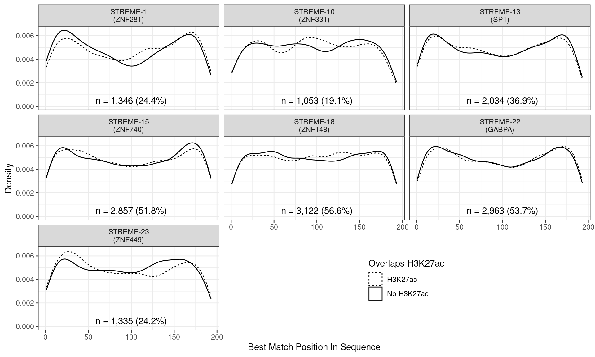
Position of the best match for each novel, H3K27ac-enriched motif using sequences centred at the summits of AR binding sites. Solid lines denote sites where H3K27ac signal was detected, whilst dashed lines indicate no H3K27ac activity. Numbers at the bottom of each panel indicate the total number of sites with a match within the AR sites overlapping H3K27ac signal.
Across all novel motifs no discernible difference was noticed in the positional distribution between sites showing H3K27ac signal and those not. However clear positional effects were evident for some of these motifs in relation to the AR binding peak.
FOXA1
streme_foxa1_summits <- streme_all4_by_h3k27ac %>%
  dplyr::slice(which(streme_to_keep_all4_by_h3k27ac)) %>%
  to_list %>%
  lapply(
    getBestMatch,
    subject = views_foxa1_summits,
    min.score = min_score
  ) %>%
  setNames(
    streme_all4_by_h3k27ac$altname[streme_to_keep_all4_by_h3k27ac]
  ) %>%
  bind_rows(.id = "altname") %>%
  dplyr::rename(range = view_name) %>%
  left_join(as_tibble(foxa1_summits), by = "range") %>%
  arrange(view) %>%
  dplyr::select(
    range, all_of(targets), H3K27ac, altname,
    pos = start_in_view, width, strand, seq
  ) %>%
  left_join(
    tomtom_all4_by_h3k27ac[streme_to_keep_all4_by_h3k27ac] %>%
      bind_rows() %>%
      dplyr::select(altname, best_match = best_match_altname),
    by = "altname"
  )
streme_foxa1_summits %>%
mutate(
label = glue("{altname}\n({best_match})"),
H3K27ac = ifelse(H3K27ac, "H3K27ac", "No H3K27ac")
) %>%
ggplot(aes(pos, stat(density))) +
geom_density(aes(linetype = H3K27ac)) +
geom_text(
aes(x = seq_width/2, y = 5e-4, label = lab),
data = . %>%
dplyr::filter(H3K27ac == "H3K27ac") %>%
group_by(label) %>%
summarise(
n = dplyr::n(), .groups = "drop"
) %>%
mutate(
lab = glue(
"n = {comma(n)} ({percent(n/sum(foxa1_summits$H3K27ac), 0.1)})"
)
),
colour = "black",
inherit.aes = FALSE
) +
facet_wrap(~ label) +
scale_linetype_manual(values = c(3, 1)) +
labs(
x = "Best Match Position In Sequence",
y = "Density",
linetype = "Overlaps H3K27ac"
) +
theme(
legend.position = c(2/3, 1/6)
)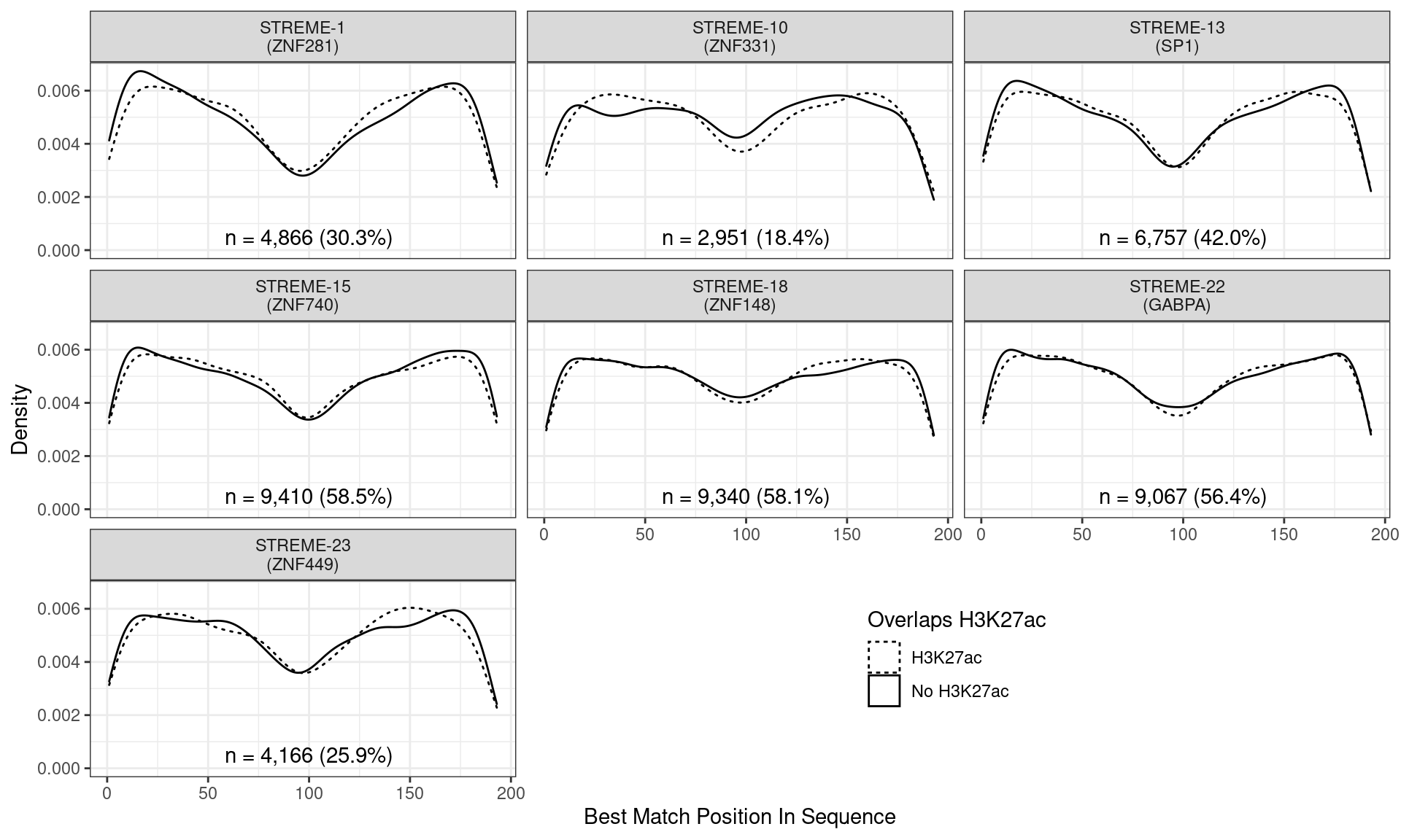
Position of the best match for each novel, H3K27ac-enriched motif using sequences centred at the summits of FOXA1 binding sites. Solid lines denote sites where H3K27ac signal was detected, whilst dashed lines indicate no H3K27ac activity. Numbers at the bottom of each panel indicate the total number of sites with a match within the FOXA1 sites overlapping H3K27ac signal.
Across all novel motifs no discernible difference was noticed in the positional distribution between sites showing H3K27ac signal and those not. However clear positional effects were evident for all these motifs in relation to the FOXA1 binding peak.
GATA3
streme_gata3_summits <- streme_all4_by_h3k27ac %>%
  dplyr::slice(which(streme_to_keep_all4_by_h3k27ac)) %>%
  to_list %>%
  lapply(
    getBestMatch,
    subject = views_gata3_summits,
    min.score = min_score
  ) %>%
  setNames(
    streme_all4_by_h3k27ac$altname[streme_to_keep_all4_by_h3k27ac]
  ) %>%
  bind_rows(.id = "altname") %>%
  dplyr::rename(range = view_name) %>%
  left_join(as_tibble(gata3_summits), by = "range") %>%
  arrange(view) %>%
  dplyr::select(
    range, all_of(targets), H3K27ac, altname,
    pos = start_in_view, width, strand, seq
  ) %>%
  left_join(
    tomtom_all4_by_h3k27ac[streme_to_keep_all4_by_h3k27ac] %>%
      bind_rows() %>%
      dplyr::select(altname, best_match = best_match_altname),
    by = "altname"
  )
streme_gata3_summits %>%
mutate(
label = glue("{altname}\n({best_match})"),
H3K27ac = ifelse(H3K27ac, "H3K27ac", "No H3K27ac")
) %>%
ggplot(aes(pos, stat(density))) +
geom_density(aes(linetype = H3K27ac)) +
geom_text(
aes(x = seq_width/2, y = 5e-4, label = lab),
data = . %>%
dplyr::filter(H3K27ac == "H3K27ac") %>%
group_by(label) %>%
summarise(
n = dplyr::n(), .groups = "drop"
) %>%
mutate(
lab = glue(
"n = {comma(n)} ({percent(n/sum(gata3_summits$H3K27ac), 0.1)})"
)
),
colour = "black",
inherit.aes = FALSE
) +
facet_wrap(~ label) +
scale_linetype_manual(values = c(3, 1)) +
labs(
x = "Best Match Position In Sequence",
y = "Density",
linetype = "Overlaps H3K27ac"
) +
theme(
legend.position = c(2/3, 1/6)
)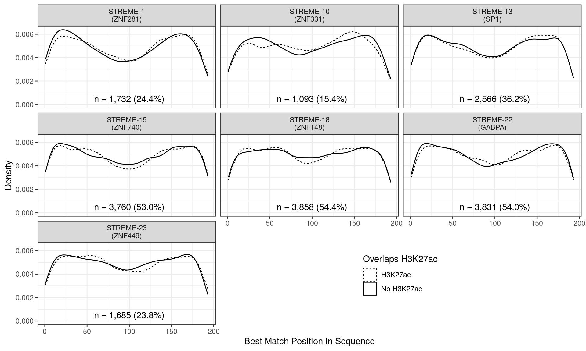
Position of the best match for each novel, H3K27ac-enriched motif using sequences centred at the summits of GATA3 binding sites. Solid lines denote sites where H3K27ac signal was detected, whilst dashed lines indicate no H3K27ac activity. Numbers at the bottom of each panel indicate the total number of sites with a match within the GATA3 sites overlapping H3K27ac signal.
Across all novel motifs no discernible difference was noticed in the positional distribution between sites showing H3K27ac signal and those not. However clear positional effects were evident for some these motifs in relation to the GATA3 binding peak.
TFAP2B
streme_tfap2b_summits <- streme_all4_by_h3k27ac %>%
  dplyr::slice(which(streme_to_keep_all4_by_h3k27ac)) %>%
  to_list %>%
  lapply(
    getBestMatch,
    subject = views_tfap2b_summits,
    min.score = min_score
  ) %>%
  setNames(
    streme_all4_by_h3k27ac$altname[streme_to_keep_all4_by_h3k27ac]
  ) %>%
  bind_rows(.id = "altname") %>%
  dplyr::rename(range = view_name) %>%
  left_join(as_tibble(tfap2b_summits), by = "range") %>%
  arrange(view) %>%
  dplyr::select(
    range, all_of(targets), H3K27ac, altname,
    pos = start_in_view, width, strand, seq
  ) %>%
  left_join(
    tomtom_all4_by_h3k27ac[streme_to_keep_all4_by_h3k27ac] %>%
      bind_rows() %>%
      dplyr::select(altname, best_match = best_match_altname),
    by = "altname"
  )
streme_tfap2b_summits %>%
mutate(
label = glue("{altname}\n({best_match})"),
H3K27ac = ifelse(H3K27ac, "H3K27ac", "No H3K27ac")
) %>%
ggplot(aes(pos, stat(density))) +
geom_density(aes(linetype = H3K27ac)) +
geom_text(
aes(x = seq_width/2, y = 5e-4, label = lab),
data = . %>%
dplyr::filter(H3K27ac == "H3K27ac") %>%
group_by(label) %>%
summarise(
n = dplyr::n(), .groups = "drop"
) %>%
mutate(
lab = glue(
"n = {comma(n)} ({percent(n/sum(tfap2b_summits$H3K27ac), 0.1)})"
)
),
colour = "black",
inherit.aes = FALSE
) +
facet_wrap(~ label) +
scale_linetype_manual(values = c(3, 1)) +
labs(
x = "Best Match Position In Sequence",
y = "Density",
linetype = "Overlaps H3K27ac"
) +
theme(
legend.position = c(2/3, 1/6)
)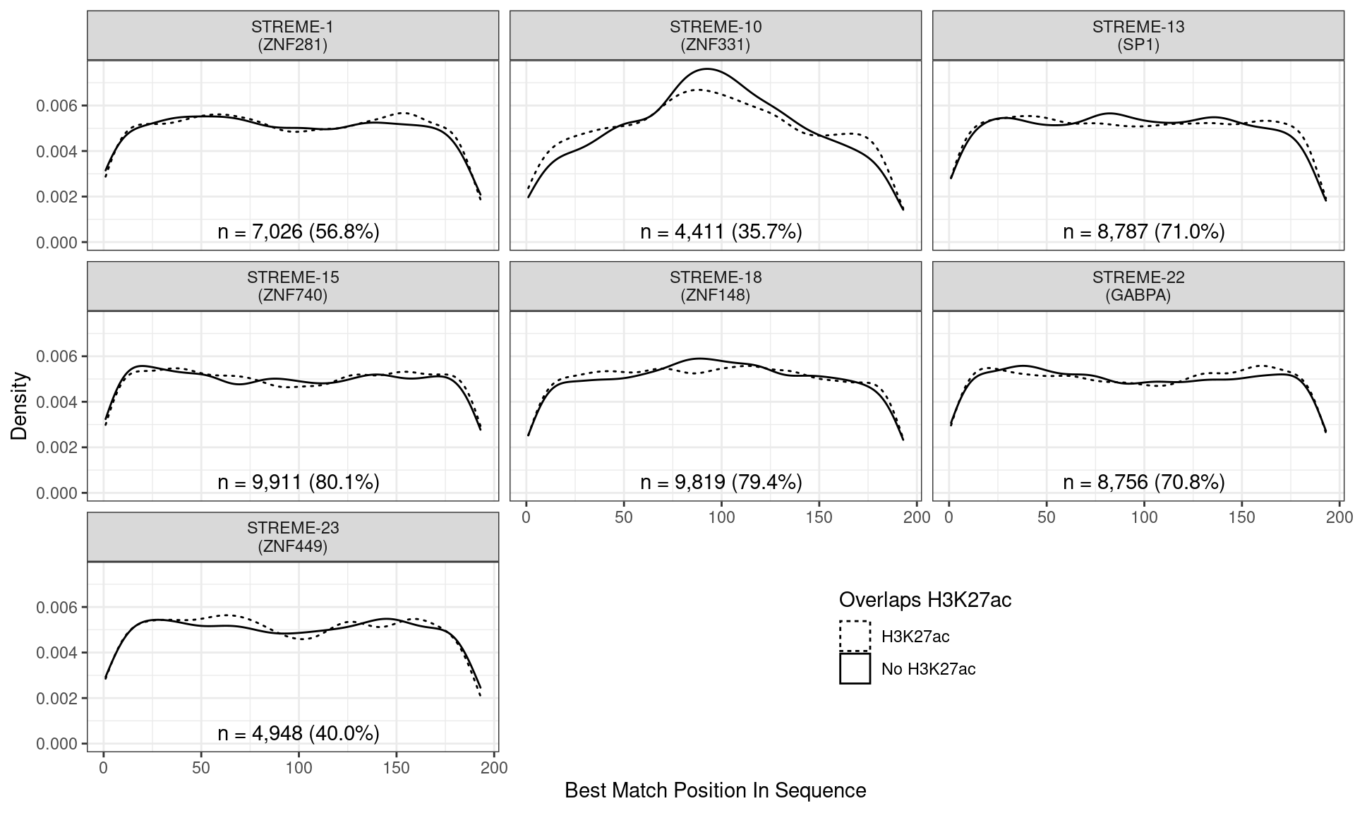
Position of the best match for each novel, H3K27ac-enriched motif using sequences centred at the summits of TFAP2B binding sites. Solid lines denote sites where H3K27ac signal was detected, whilst dashed lines indicate no H3K27ac activity. Numbers at the bottom of each panel indicate the total number of sites with a match within the TFAP2B sites overlapping H3K27ac signal.
Across all novel motifs no discernible difference was noticed in the positional distribution between sites showing H3K27ac signal and those not. However clear positional effects were evident for all these motifs in relation to the TFAP2B binding peak.
sessionInfo()R version 4.2.0 (2022-04-22)
Platform: x86_64-pc-linux-gnu (64-bit)
Running under: Ubuntu 20.04.4 LTS
Matrix products: default
BLAS: /usr/lib/x86_64-linux-gnu/blas/libblas.so.3.9.0
LAPACK: /usr/lib/x86_64-linux-gnu/lapack/liblapack.so.3.9.0
locale:
[1] LC_CTYPE=en_AU.UTF-8 LC_NUMERIC=C
[3] LC_TIME=en_AU.UTF-8 LC_COLLATE=en_AU.UTF-8
[5] LC_MONETARY=en_AU.UTF-8 LC_MESSAGES=en_AU.UTF-8
[7] LC_PAPER=en_AU.UTF-8 LC_NAME=C
[9] LC_ADDRESS=C LC_TELEPHONE=C
[11] LC_MEASUREMENT=en_AU.UTF-8 LC_IDENTIFICATION=C
attached base packages:
[1] parallel stats4 stats graphics grDevices utils datasets
[8] methods base
other attached packages:
[1] gt_0.6.0 cowplot_1.1.1
[3] glue_1.6.2 pander_0.6.5
[5] scales_1.2.0 BSgenome.Hsapiens.UCSC.hg19_1.4.3
[7] BSgenome_1.64.0 Biostrings_2.64.0
[9] XVector_0.36.0 magrittr_2.0.3
[11] rtracklayer_1.56.0 extraChIPs_1.0.0
[13] SummarizedExperiment_1.26.1 Biobase_2.56.0
[15] MatrixGenerics_1.8.0 matrixStats_0.62.0
[17] BiocParallel_1.30.2 plyranges_1.16.0
[19] GenomicRanges_1.48.0 GenomeInfoDb_1.32.2
[21] IRanges_2.30.0 S4Vectors_0.34.0
[23] BiocGenerics_0.42.0 forcats_0.5.1
[25] stringr_1.4.0 dplyr_1.0.9
[27] purrr_0.3.4 readr_2.1.2
[29] tidyr_1.2.0 tibble_3.1.7
[31] ggplot2_3.3.6 tidyverse_1.3.1
[33] universalmotif_1.14.0 memes_1.4.1
[35] workflowr_1.7.0
loaded via a namespace (and not attached):
[1] rappdirs_0.3.3 R.methodsS3_1.8.1
[3] csaw_1.30.1 bit64_4.0.5
[5] knitr_1.39 DelayedArray_0.22.0
[7] R.utils_2.11.0 data.table_1.14.2
[9] rpart_4.1.16 KEGGREST_1.36.0
[11] RCurl_1.98-1.6 AnnotationFilter_1.20.0
[13] doParallel_1.0.17 generics_0.1.2
[15] GenomicFeatures_1.48.1 callr_3.7.0
[17] EnrichedHeatmap_1.26.0 usethis_2.1.6
[19] RSQLite_2.2.14 commonmark_1.8.0
[21] bit_4.0.4 tzdb_0.3.0
[23] xml2_1.3.3 lubridate_1.8.0
[25] httpuv_1.6.5 assertthat_0.2.1
[27] xfun_0.31 hms_1.1.1
[29] jquerylib_0.1.4 evaluate_0.15
[31] promises_1.2.0.1 fansi_1.0.3
[33] restfulr_0.0.13 progress_1.2.2
[35] dbplyr_2.1.1 readxl_1.4.0
[37] igraph_1.3.1 DBI_1.1.2
[39] htmlwidgets_1.5.4 ellipsis_0.3.2
[41] backports_1.4.1 biomaRt_2.52.0
[43] vctrs_0.4.1 here_1.0.1
[45] ensembldb_2.20.1 cachem_1.0.6
[47] withr_2.5.0 ggforce_0.3.3
[49] Gviz_1.40.1 checkmate_2.1.0
[51] vroom_1.5.7 GenomicAlignments_1.32.0
[53] prettyunits_1.1.1 cluster_2.1.3
[55] lazyeval_0.2.2 crayon_1.5.1
[57] edgeR_3.38.1 pkgconfig_2.0.3
[59] labeling_0.4.2 tweenr_1.0.2
[61] pkgload_1.2.4 ProtGenerics_1.28.0
[63] nnet_7.3-17 rlang_1.0.2
[65] lifecycle_1.0.1 filelock_1.0.2
[67] BiocFileCache_2.4.0 modelr_0.1.8
[69] dichromat_2.0-0.1 cellranger_1.1.0
[71] rprojroot_2.0.3 polyclip_1.10-0
[73] Matrix_1.4-1 ggseqlogo_0.1
[75] reprex_2.0.1 base64enc_0.1-3
[77] whisker_0.4 GlobalOptions_0.1.2
[79] processx_3.5.3 png_0.1-7
[81] rjson_0.2.21 GenomicInteractions_1.30.0
[83] bitops_1.0-7 cmdfun_1.0.2
[85] getPass_0.2-2 R.oo_1.24.0
[87] blob_1.2.3 shape_1.4.6
[89] jpeg_0.1-9 memoise_2.0.1
[91] zlibbioc_1.42.0 compiler_4.2.0
[93] scatterpie_0.1.7 BiocIO_1.6.0
[95] RColorBrewer_1.1-3 clue_0.3-60
[97] Rsamtools_2.12.0 cli_3.3.0
[99] ps_1.7.0 htmlTable_2.4.0
[101] Formula_1.2-4 MASS_7.3-56
[103] ggside_0.2.0.9990 tidyselect_1.1.2
[105] stringi_1.7.6 highr_0.9
[107] yaml_2.3.5 locfit_1.5-9.5
[109] latticeExtra_0.6-29 ggrepel_0.9.1
[111] grid_4.2.0 sass_0.4.1
[113] VariantAnnotation_1.42.1 tools_4.2.0
[115] circlize_0.4.15 rstudioapi_0.13
[117] foreach_1.5.2 foreign_0.8-82
[119] git2r_0.30.1 metapod_1.4.0
[121] gridExtra_2.3 farver_2.1.0
[123] digest_0.6.29 Rcpp_1.0.8.3
[125] broom_0.8.0 later_1.3.0
[127] httr_1.4.3 AnnotationDbi_1.58.0
[129] biovizBase_1.44.0 ComplexHeatmap_2.12.0
[131] colorspace_2.0-3 rvest_1.0.2
[133] brio_1.1.3 XML_3.99-0.9
[135] fs_1.5.2 splines_4.2.0
[137] jsonlite_1.8.0 ggfun_0.0.6
[139] testthat_3.1.4 R6_2.5.1
[141] Hmisc_4.7-0 pillar_1.7.0
[143] htmltools_0.5.2 fastmap_1.1.0
[145] codetools_0.2-18 utf8_1.2.2
[147] lattice_0.20-45 bslib_0.3.1
[149] curl_4.3.2 survival_3.2-13
[151] limma_3.52.1 rmarkdown_2.14
[153] InteractionSet_1.24.0 desc_1.4.1
[155] munsell_0.5.0 GetoptLong_1.0.5
[157] GenomeInfoDbData_1.2.8 iterators_1.0.14
[159] haven_2.5.0 gtable_0.3.0