Summary of WP1 data products for FACE-IT study sites
Robert Schlegel
21 septembre 2021
Last updated: 2021-09-21
Checks: 7 0
Knit directory: WP1/
This reproducible R Markdown analysis was created with workflowr (version 1.6.2). The Checks tab describes the reproducibility checks that were applied when the results were created. The Past versions tab lists the development history.
Great! Since the R Markdown file has been committed to the Git repository, you know the exact version of the code that produced these results.
Great job! The global environment was empty. Objects defined in the global environment can affect the analysis in your R Markdown file in unknown ways. For reproduciblity it’s best to always run the code in an empty environment.
The command set.seed(20210216) was run prior to running the code in the R Markdown file. Setting a seed ensures that any results that rely on randomness, e.g. subsampling or permutations, are reproducible.
Great job! Recording the operating system, R version, and package versions is critical for reproducibility.
Nice! There were no cached chunks for this analysis, so you can be confident that you successfully produced the results during this run.
Great job! Using relative paths to the files within your workflowr project makes it easier to run your code on other machines.
Great! You are using Git for version control. Tracking code development and connecting the code version to the results is critical for reproducibility.
The results in this page were generated with repository version b966f85. See the Past versions tab to see a history of the changes made to the R Markdown and HTML files.
Note that you need to be careful to ensure that all relevant files for the analysis have been committed to Git prior to generating the results (you can use wflow_publish or wflow_git_commit). workflowr only checks the R Markdown file, but you know if there are other scripts or data files that it depends on. Below is the status of the Git repository when the results were generated:
Ignored files:
    Ignored:    .Rhistory
    Ignored:    .Rproj.user/
    Ignored:    code/ny-alesund_cc_pf_rws.R
    Ignored:    data/model/
    Ignored:    data/pg_data/
    Ignored:    metadata/pangaea_parameters.tab

Unstaged changes:
    Modified:   code/functions.R
Note that any generated files, e.g. HTML, png, CSS, etc., are not included in this status report because it is ok for generated content to have uncommitted changes.
These are the previous versions of the repository in which changes were made to the R Markdown (analysis/data_summary.Rmd) and HTML (docs/data_summary.html) files. If you’ve configured a remote Git repository (see ?wflow_git_remote), click on the hyperlinks in the table below to view the files as they were in that past version.
| File | Version | Author | Date | Message |
|---|---|---|---|---|
| Rmd | ed8e079 | Robert | 2021-09-21 | Updated data summary page |
| html | ed8e079 | Robert | 2021-09-21 | Updated data summary page |
| Rmd | 32b5b93 | Robert | 2021-09-15 | Considering adding model summaries to data summary page. |
| html | 32b5b93 | Robert | 2021-09-15 | Considering adding model summaries to data summary page. |
| Rmd | 1caac63 | Robert | 2021-09-15 | Updates to WP1 website |
| html | 1caac63 | Robert | 2021-09-15 | Updates to WP1 website |
| html | dd71077 | Robert | 2021-09-07 | Update to summary figures. Now using hi-res coastlines. |
| Rmd | b4d9162 | Robert | 2021-08-25 | Completed touch-ups to all of the summary figures |
| html | b4d9162 | Robert | 2021-08-25 | Completed touch-ups to all of the summary figures |
| Rmd | 0edbfc5 | Robert | 2021-08-24 | Cleaning up summary functions and figures |
| html | 0edbfc5 | Robert | 2021-08-24 | Cleaning up summary functions and figures |
| Rmd | 018987f | Robert | 2021-08-18 | First draft of trend summaries |
| html | 018987f | Robert | 2021-08-18 | First draft of trend summaries |
| Rmd | aac779d | Robert | 2021-08-18 | First draft of climatology summaries added |
| html | aac779d | Robert | 2021-08-18 | First draft of climatology summaries added |
| Rmd | 90cda7b | Robert | 2021-08-18 | First draft of data summary page |
| html | 90cda7b | Robert | 2021-08-18 | First draft of data summary page |
| Rmd | 2136a33 | Robert | 2021-08-17 | Addressed the issue of sub-daily data |
| html | 36454cc | Robert | 2021-08-17 | Build site. |
| Rmd | 438add7 | Robert | 2021-08-17 | Re-built site. |
Overview
This document contains a summary of the data products produced for WP1 of the FACE-IT project. These data are available to all FACE-IT members via password protected pCloud access. These data are also used in the meta-analysis review of the key drivers of change to arctic fjord ecosystems, which is a 24 month (October, 2022) deliverable.
Svalbard
Kongsfjorden
High level summary of data available for Kongsfjorden.
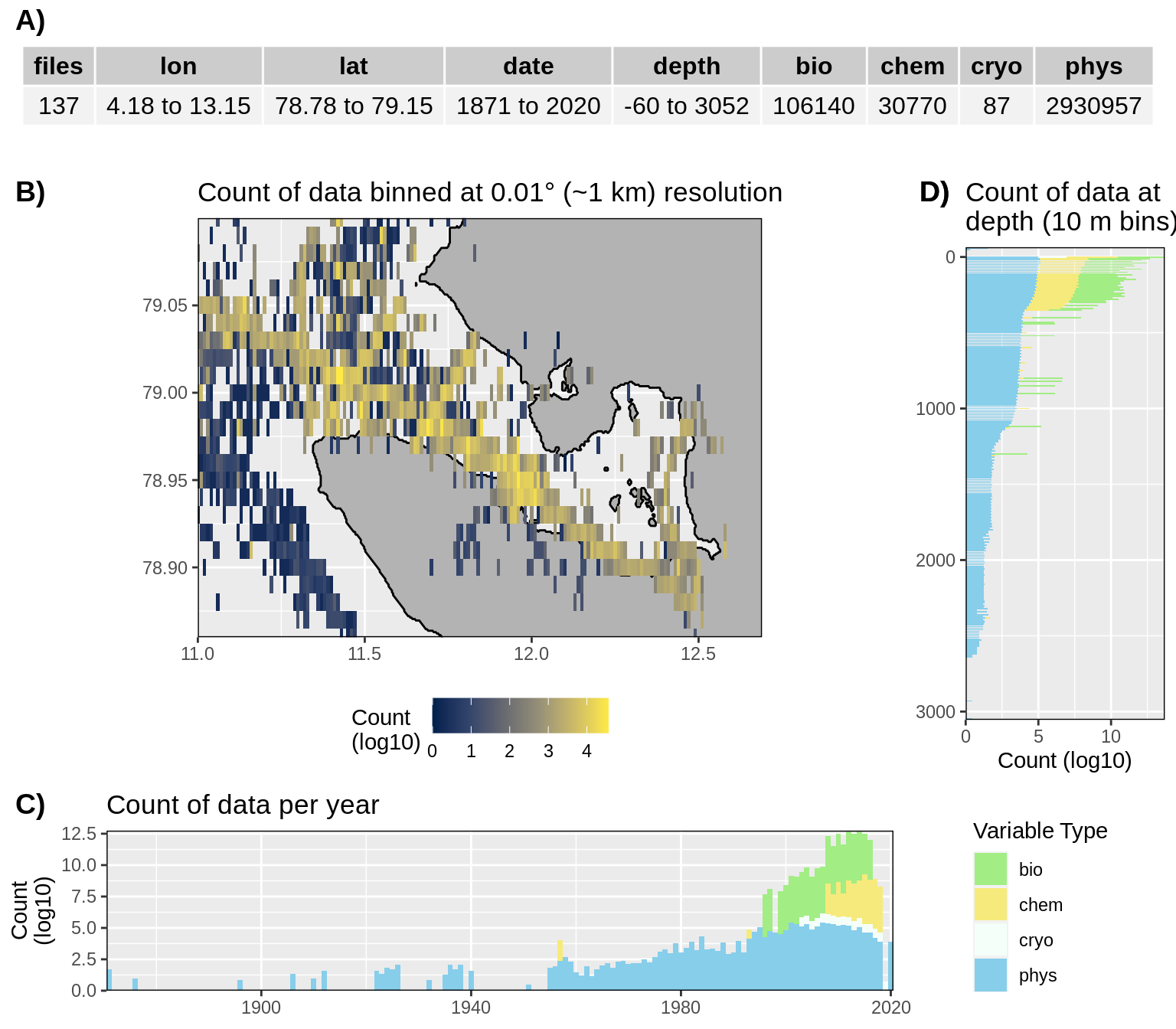
Figure 1: High level overview of the data available for Kongsfjorden. The acronyms for the variable groups seen throughout the figure are: bio = biology, chem = chemistry, cryo = cryosphere, phys = physical, soc = social (currently there are no social data for Kongsfjorden). A) Metadata showing the range of values available within the data. B) Spatial summary of data available per ~1 km grouping. C) Temporal summary of available data. D) Summmary of data available by depth. Note that all of the data summaries are log10 transformed. For C) and D) the log10 transformation is applied before the data are stacked by category, which gives the impression that there are much more data are than there are.
Monthly average values for temperature and salinity data. These are taken as illustrative figures for the data that are likely available per month as they are generally the two most highly sampled variables in marine science.
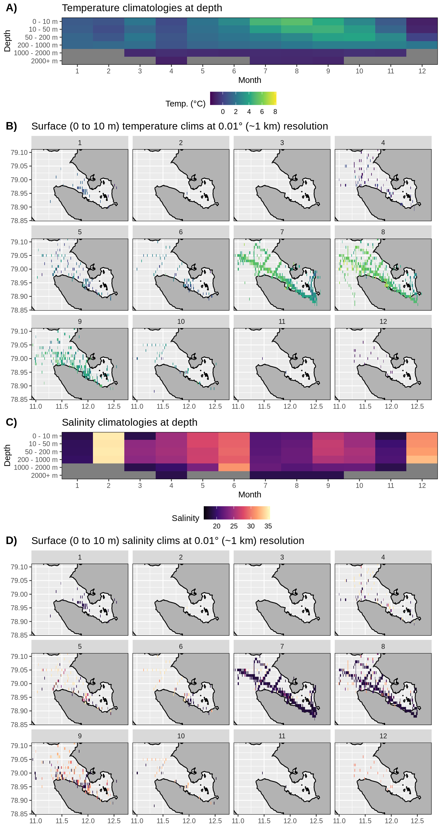
Figure 2: Monthly climatologies for data at Kongsfjorden. The entire range of data was used for the climatology period. A) Temperature climatolgies at depths for all of Kongsfjorden. B) Spatial surface (0 to 10 m) temperature climatologies. C) Salinity climatologies at depth for all of Kongsfjorden. Note the much higher salinity for February and how most of the values are much lower than would be assumed. Probably due to a different sort of salinity calculation being used. D) Spatial surface (0 to 10 m) salinity climatologies.
Trends in temperature and salinity data.
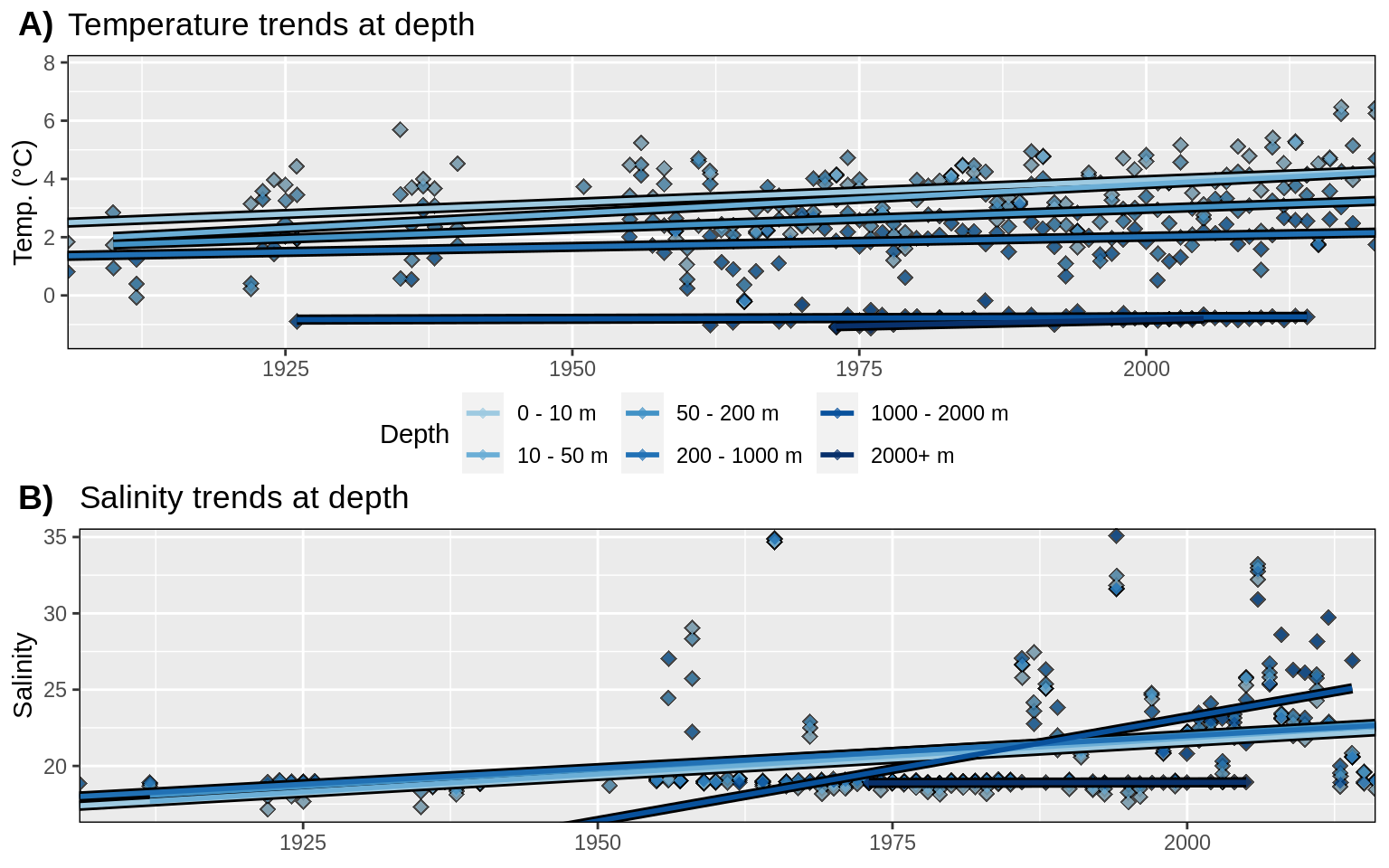
Figure 3: Trends in A) temperature and B) salinity at different depth groups. The average annual values for all data are shown as diamonds, and the annual trends for these values are shown as coloured lines. There also appear to be two different types of salinity measurements. A long record of values close to 20 and a more recent addition of higher values around 32-35. One assumes that the lower values are measures of runoff and not proper ocean water.
Isfjorden
High level summary of data available for Isfjorden.
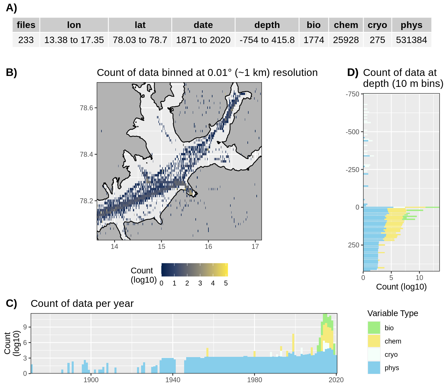
Figure 4: High level overview of the data available for Isfjorden. The acronyms for the variable groups seen throughout the figure are: bio = biology, chem = chemistry, cryo = cryosphere, phys = physical, soc = social (currently there are no social data for Isfjorden). A) Metadata showing the range of values available within the data. B) Spatial summary of data available per ~1 km grouping. Note that there are some important moorings outside of this bounding box that are included in the data counts. C) Temporal summary of available data. D) Summmary of data available by depth. Note that all of the data summaries are log10 transformed. For C) and D) the log10 transformation is applied before the data are stacked by category, which gives the impression that there are much more data are than there are.
Monthly average values for temperature and salinity data.
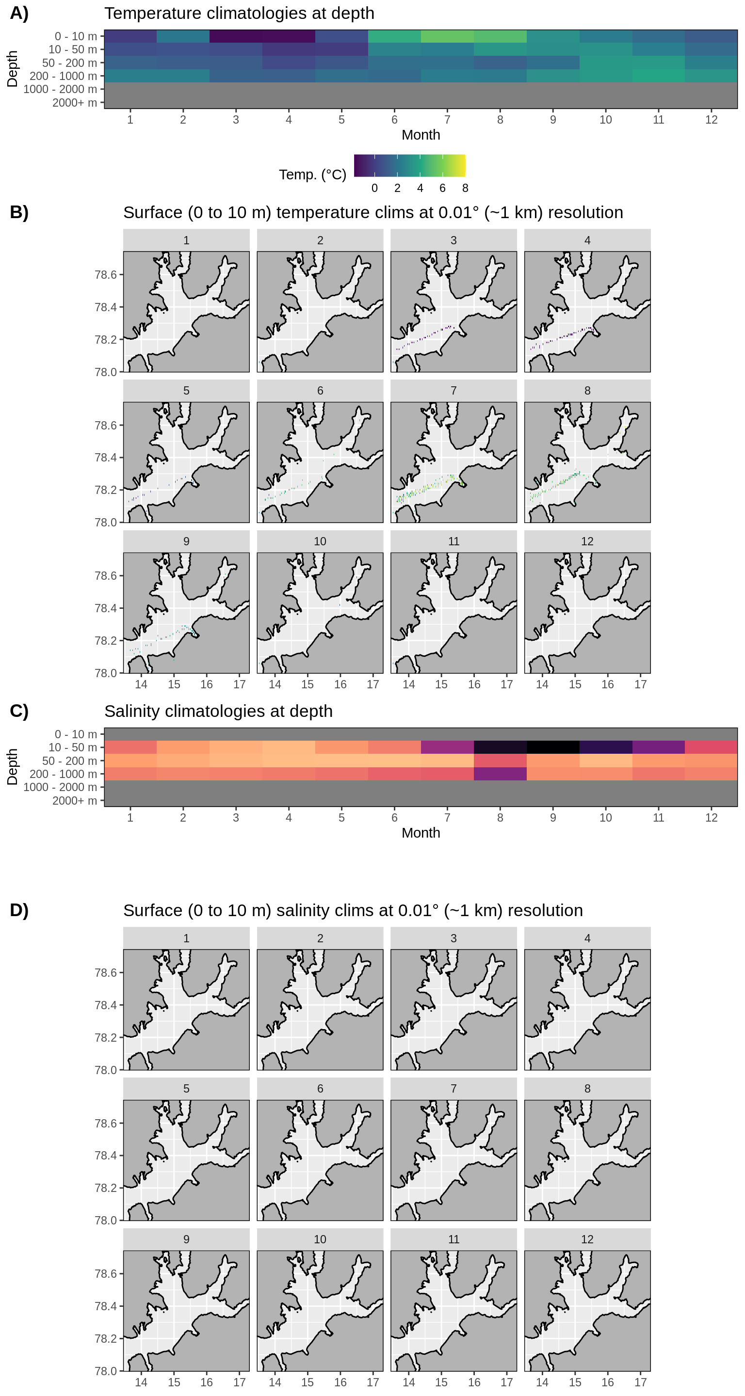
Figure 5: Monthly climatologies for data at Isfjorden. The entire range of data was used for the climatology period. A) Temperature climatolgies at depths for all of Isfjorden. B) Spatial surface (0 to 10 m) temperature climatologies. C) Salinity climatologies at depth for all of Isfjorden. D) Spatial surface (0 to 10 m) salinity climatologies. Note that there are no surface salinity values for Isfjorden within the bounding box.
Trends in temperature and salinity data.
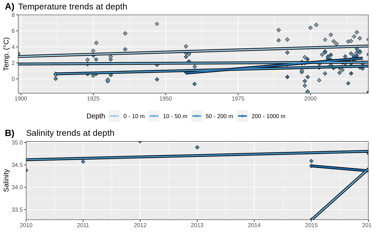
Figure 6: Trends in A) temperature and B) salinity at different depth groups. The average annual values for all data are shown as diamonds, and the annual trends for these values are shown as coloured lines. Note that there are not currently many salinity data points for Isfjorden.
Inglefieldbukta
High level summary of data available for Inglefieldbukta.
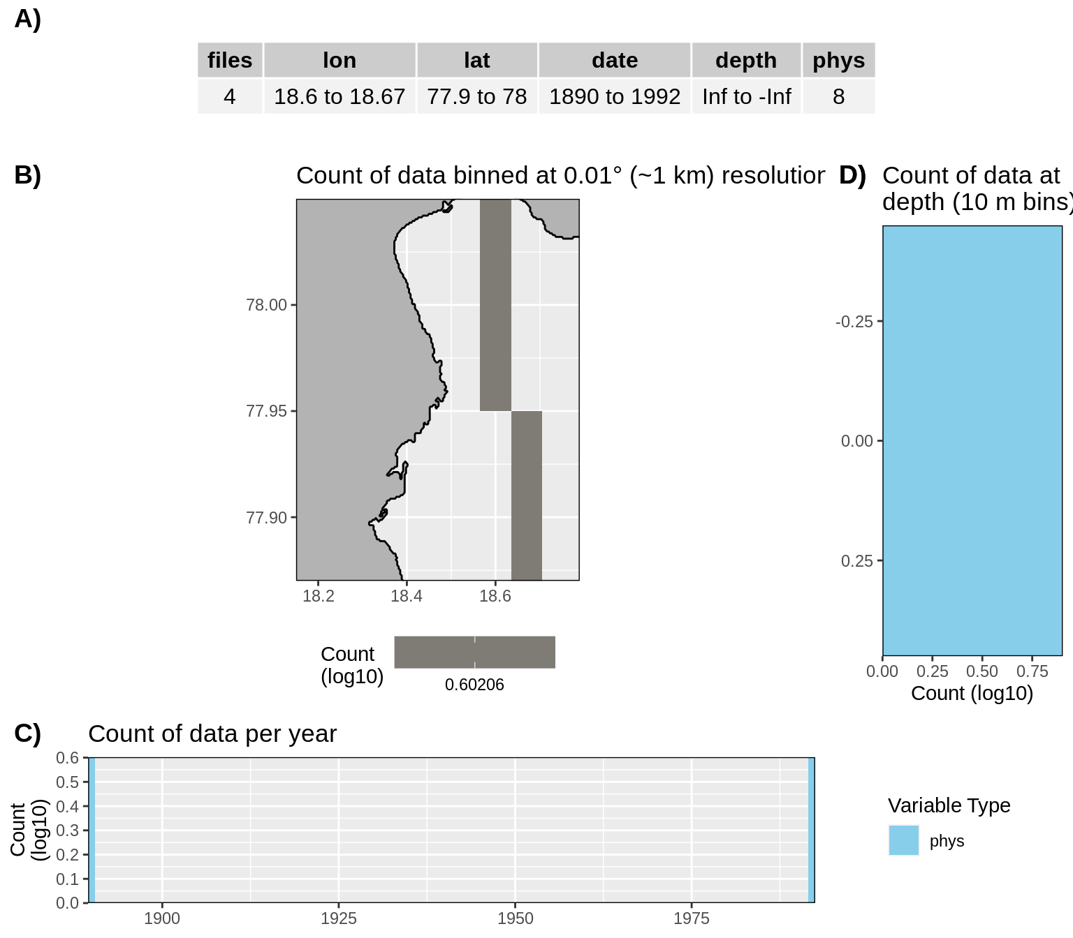
Figure 7: High level overview of the data available for Inglefieldbukta. The acronyms for the variable groups seen throughout the figure are: bio = biology, chem = chemistry, cryo = cryosphere, phys = physical, soc = social (currently there are only physical data for Inglefieldbukta). A) Metadata showing the range of values available within the data. B) Spatial summary of data available per ~1 km grouping. Note that there are only two pixels because there are almost no data. C) Temporal summary of available data. D) Summmary of data available by depth (blank because there are no depth data). Note that all of the data summaries are log10 transformed.
Monthly average values for temperature and salinity data.

Figure 8: Not enough data exist to calculate climatologies.
| Version | Author | Date |
|---|---|---|
| b4d9162 | Robert | 2021-08-25 |
Trends in temperature and salinity data.

Figure 9: Not enough data exist to calculate trends.
| Version | Author | Date |
|---|---|---|
| b4d9162 | Robert | 2021-08-25 |
Greenland
Young Sound
High level summary of data available for Young Sound.
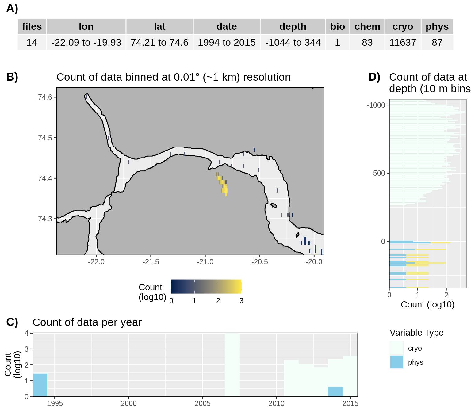
Figure 10: High level overview of the data available for Young Sound. The acronyms for the variable groups seen throughout the figure are: bio = biology, chem = chemistry, cryo = cryosphere, phys = physical, soc = social (currently there are only cryo and phys data for Young Sound). A) Metadata showing the range of values available within the data. B) Spatial summary of data available per ~1 km grouping. C) Temporal summary of available data. D) Summmary of data available by depth. Note that all of the data summaries are log10 transformed. For C) and D) the log10 transformation is applied before the data are stacked by category, which gives the impression that there are much more data are than there are.
Monthly average values for temperature and salinity data.

Figure 11: Not enough data exist to calculate trends.
| Version | Author | Date |
|---|---|---|
| b4d9162 | Robert | 2021-08-25 |
Trends in temperature and salinity data.

Figure 12: Not enough data exist to calculate trends.
| Version | Author | Date |
|---|---|---|
| b4d9162 | Robert | 2021-08-25 |
Disko Bay
High level summary of data available for Disko Bay.
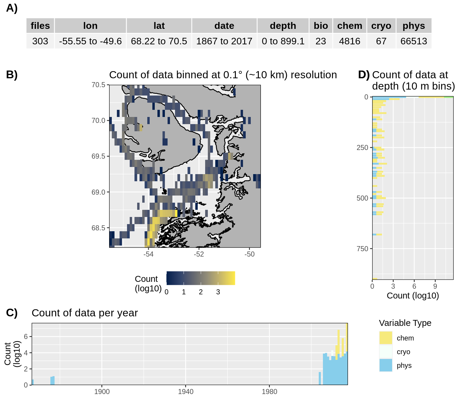
Figure 13: High level overview of the data available for Disko Bay. The acronyms for the variable groups seen throughout the figure are: bio = biology, chem = chemistry, cryo = cryosphere, phys = physical, soc = social (currently there are no bio or soc data for Disko Bay). A) Metadata showing the range of values available within the data. B) Spatial summary of data available per ~10 km grouping. C) Temporal summary of available data. D) Summmary of data available by depth. Note that all of the data summaries are log10 transformed. For C) and D) the log10 transformation is applied before the data are stacked by category, which gives the impression that there are much more data are than there are.
Monthly average values for temperature and salinity data.
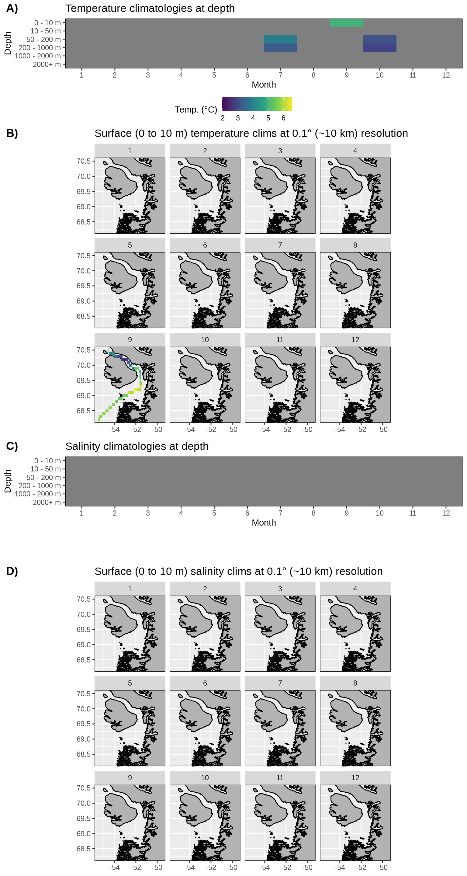
Figure 14: Monthly climatologies for data at Disko Bay. The entire range of data was used for the climatology period. A) Temperature climatolgies at depths for all of Disko Bay. B) Spatial surface (0 to 10 m) temperature climatologies. C) Salinity climatologies at depth for all of Disko Bay. D) Spatial surface (0 to 10 m) salinity climatologies. Note that there are no salinity values for Disko Bay and almost no temperature values.
Trends in temperature and salinity data.

Figure 15: Not enough data exist to calculate trends.
| Version | Author | Date |
|---|---|---|
| b4d9162 | Robert | 2021-08-25 |
Nuup Kangerlua
High level summary of data available for Nuup Kangerlua.
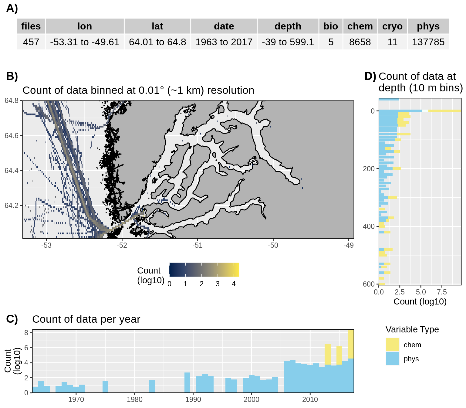
Figure 16: High level overview of the data available for Nuup Kangerlua. The acronyms for the variable groups seen throughout the figure are: bio = biology, chem = chemistry, cryo = cryosphere, phys = physical, soc = social (currently only chem and phys data are available). A) Metadata showing the range of values available within the data. B) Spatial summary of data available per ~1 km grouping. Note how almost all of the data are from outside of the fjord. C) Temporal summary of available data. D) Summmary of data available by depth. Note that all of the data summaries are log10 transformed. For C) and D) the log10 transformation is applied before the data are stacked by category, which gives the impression that there are much more data are than there are.
Monthly average values for temperature and salinity data.
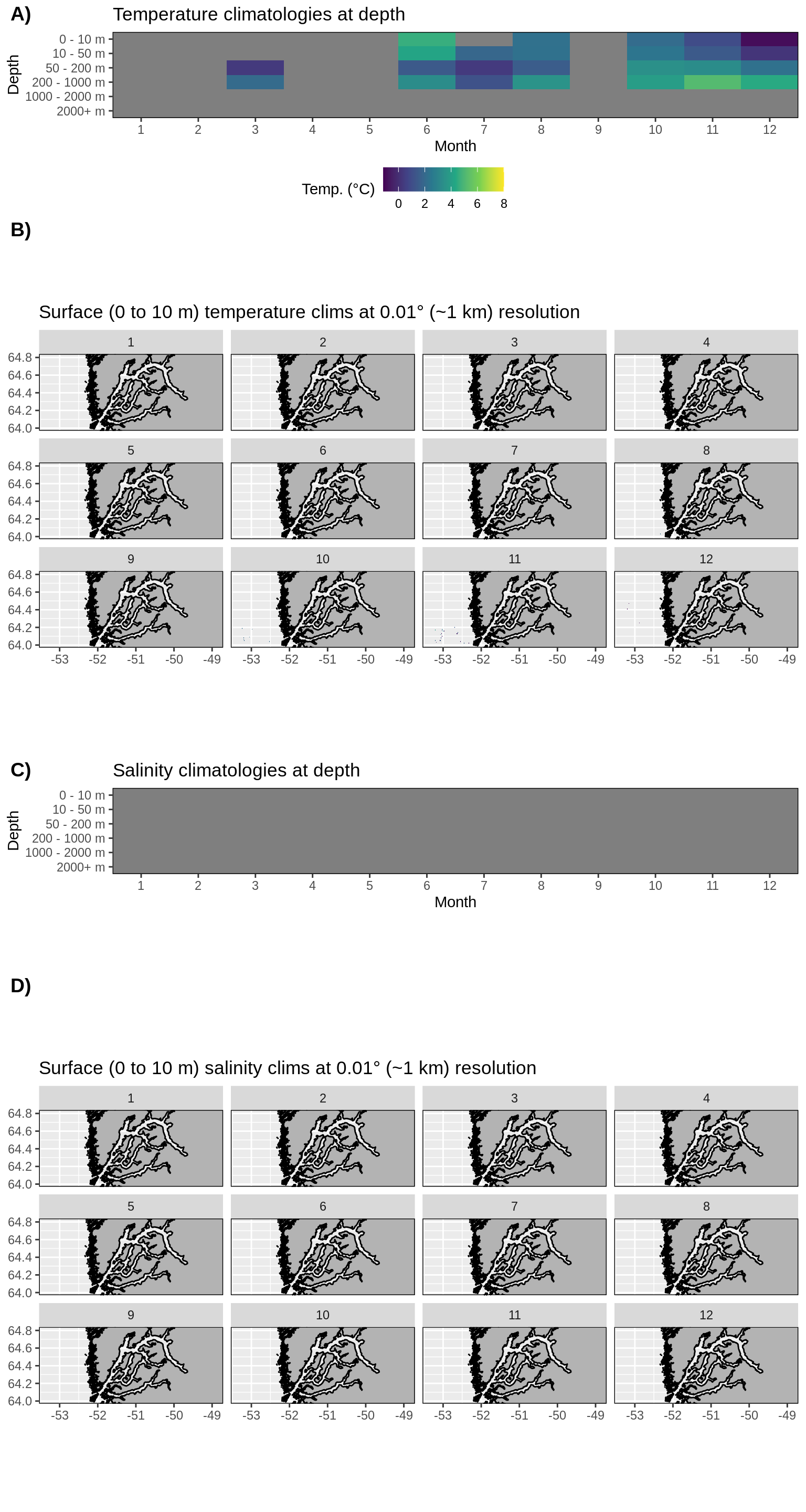
Figure 17: Monthly climatologies for data at Nuup Kangerlua. The entire range of data was used for the climatology period. A) Temperature climatolgies at depths for all of Nuup Kangerlua. B) Spatial surface (0 to 10 m) temperature climatologies. C) Salinity climatologies at depth for all of Nuup Kangerlua. D) Spatial surface (0 to 10 m) salinity climatologies. Note that there are no salinity values for Nuup Kangerlua and sparse temperature values.
Trends in temperature and salinity data.
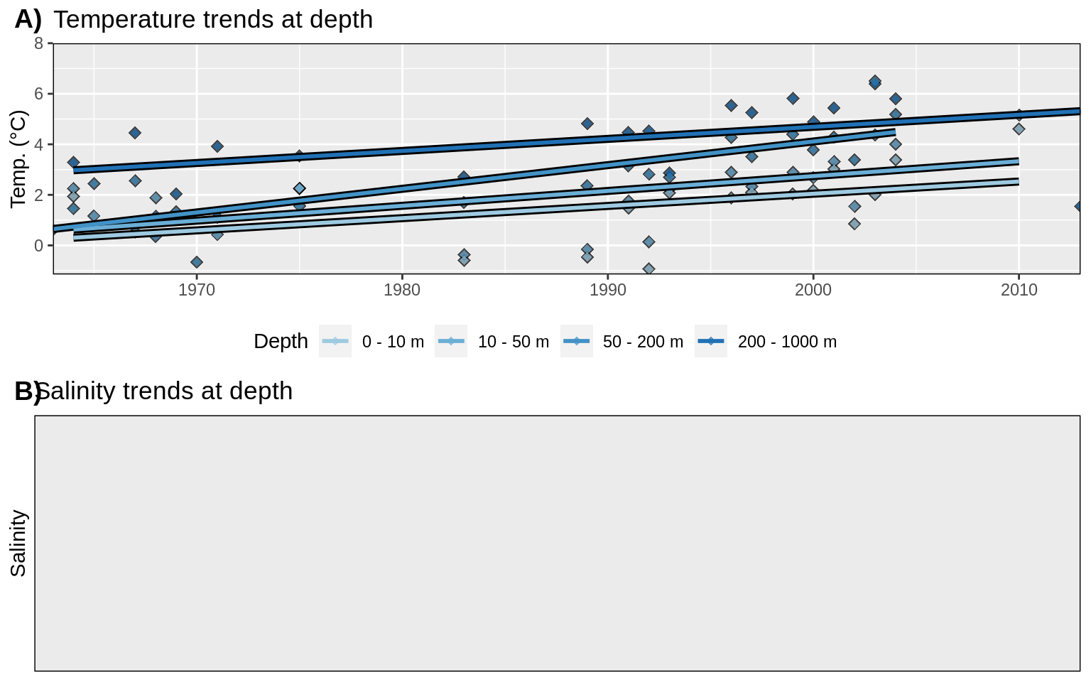
Figure 18: Trends in A) temperature and B) salinity at different depth groups. The average annual values for all data are shown as diamonds, and the annual trends for these values are shown as coloured lines. Note that there are no salinity data.
Norway
Porsangerfjorden
High level summary of data available for Porsangerfjorden.
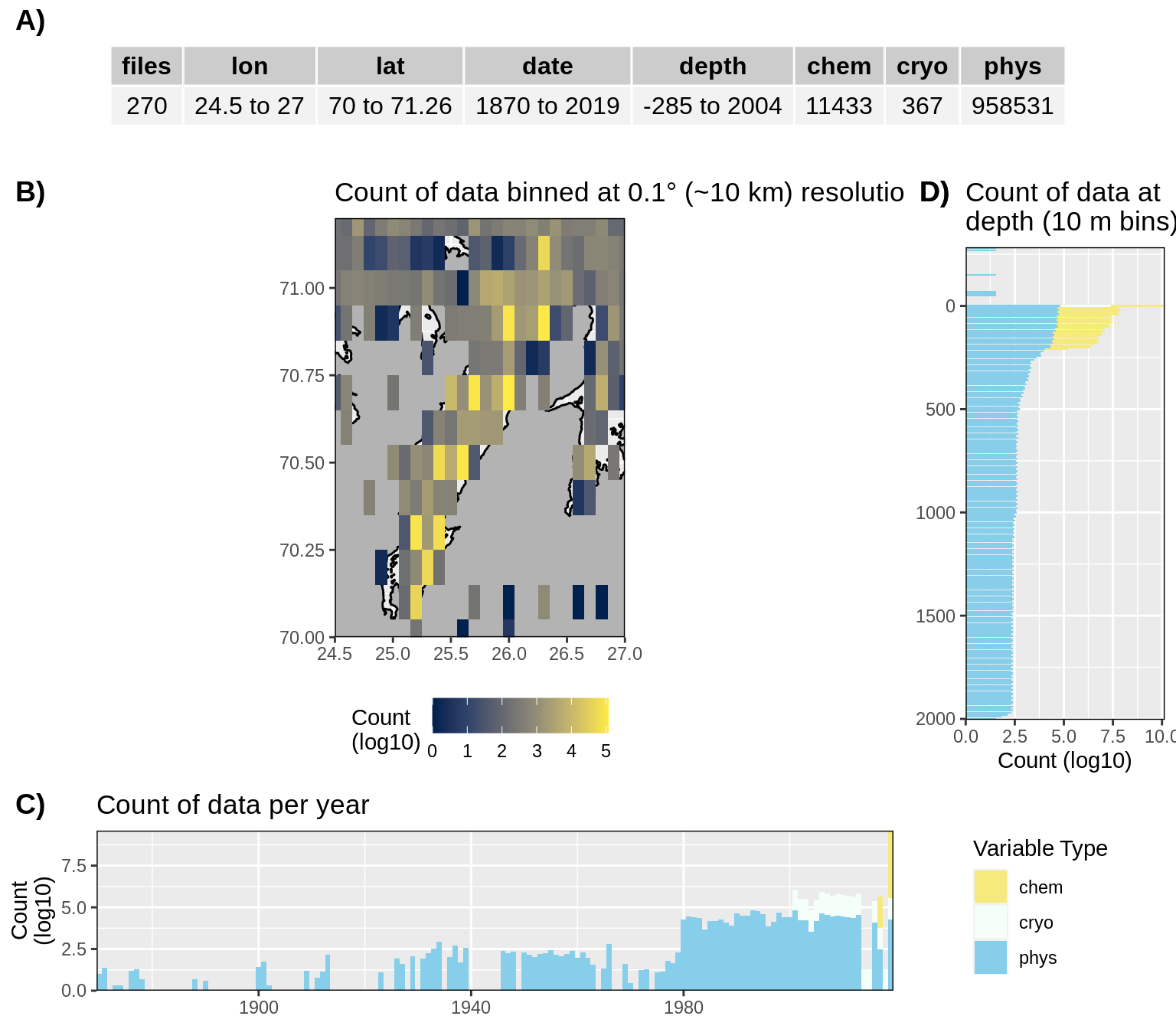
Figure 19: High level overview of the data available for Porsangerfjorden. The acronyms for the variable groups seen throughout the figure are: bio = biology, chem = chemistry, cryo = cryosphere, phys = physical, soc = social (currently only chem and phys data are available). A) Metadata showing the range of values available within the data. B) Spatial summary of data available per ~10 km grouping. Note how a lot of data are from outside of the fjord. C) Temporal summary of available data. D) Summmary of data available by depth. Note that all of the data summaries are log10 transformed. For C) and D) the log10 transformation is applied before the data are stacked by category, which gives the impression that there are much more data are than there are.
Monthly average values for temperature and salinity data.
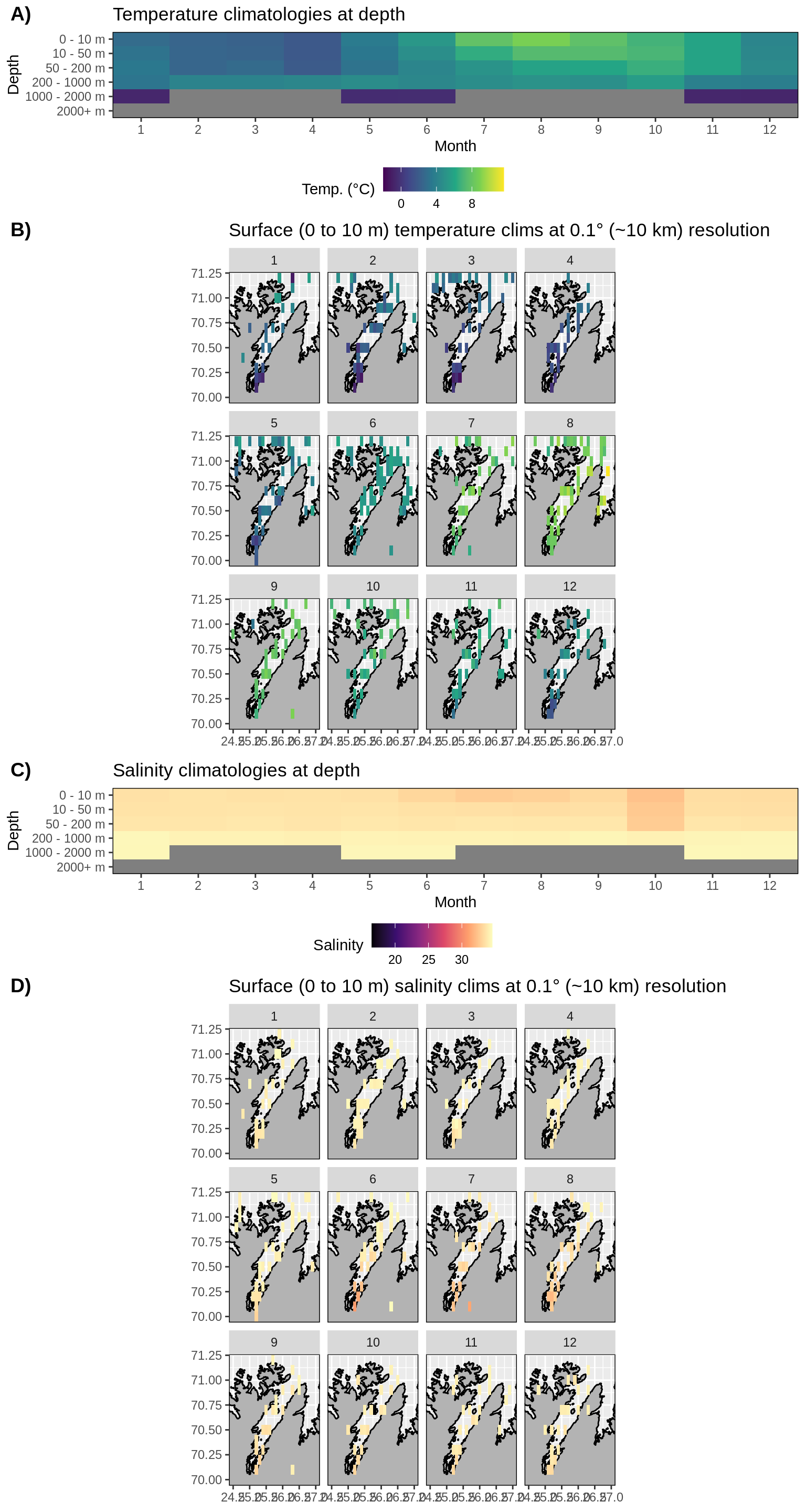
Figure 20: Monthly climatologies for data at Porsangerfjorden. The entire range of data was used for the climatology period. A) Temperature climatolgies at depths for all of Porsangerfjorden. B) Spatial surface (0 to 10 m) temperature climatologies. C) Salinity climatologies at depth for all of Porsangerfjorden. D) Spatial surface (0 to 10 m) salinity climatologies. Note that there are no surface salinity values for Porsangerfjorden and the salinity values are questionable.
Trends in temperature and salinity data.
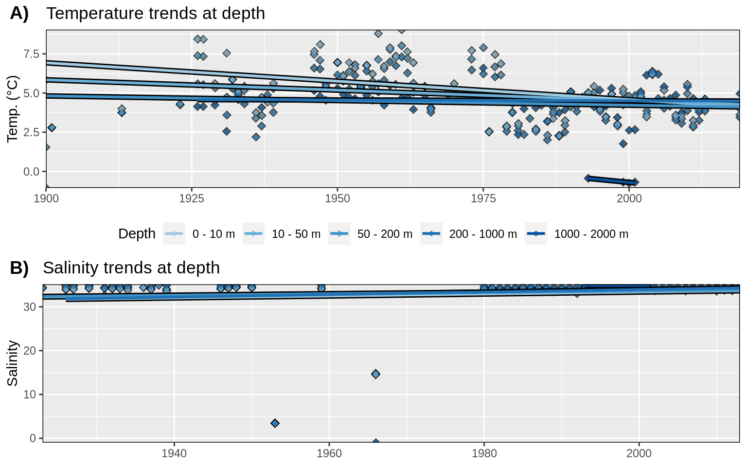
Figure 21: Trends in A) temperature and B) salinity at different depth groups. The average annual values for all data are shown as diamonds, and the annual trends for these values are shown as coloured lines. Note that there are not enough salinity data to calculate trends.
References
R version 4.1.1 (2021-08-10)
Platform: x86_64-pc-linux-gnu (64-bit)
Running under: Ubuntu 18.04.6 LTS

Matrix products: default
BLAS:   /usr/lib/x86_64-linux-gnu/blas/libblas.so.3.7.1
LAPACK: /usr/lib/x86_64-linux-gnu/lapack/liblapack.so.3.7.1

locale:
 [1] LC_CTYPE=en_GB.UTF-8       LC_NUMERIC=C
 [3] LC_TIME=fr_FR.UTF-8        LC_COLLATE=en_GB.UTF-8
 [5] LC_MONETARY=fr_FR.UTF-8    LC_MESSAGES=en_GB.UTF-8
 [7] LC_PAPER=fr_FR.UTF-8       LC_NAME=C
 [9] LC_ADDRESS=C               LC_TELEPHONE=C
[11] LC_MEASUREMENT=fr_FR.UTF-8 LC_IDENTIFICATION=C

attached base packages:
[1] parallel  grid      stats     graphics  grDevices utils     datasets
[8] methods   base

other attached packages:
 [1] doParallel_1.0.16  iterators_1.0.13   foreach_1.5.1      pangaear_1.1.0
 [5] sf_1.0-0           sp_1.4-5           RColorBrewer_1.1-2 ggOceanMaps_1.1.9
 [9] ggspatial_1.1.5    gtable_0.3.0       gridExtra_2.3      PCICt_0.5-4.1
[13] tidync_0.2.4       forcats_0.5.1      stringr_1.4.0      dplyr_1.0.6
[17] purrr_0.3.4        readr_1.4.0        tidyr_1.1.3        tibble_3.1.2
[21] ggplot2_3.3.3      tidyverse_1.3.1    workflowr_1.6.2

loaded via a namespace (and not attached):
  [1] colorspace_2.0-1   ggsignif_0.6.2     ellipsis_0.3.2
  [4] class_7.3-19       rio_0.5.26         rprojroot_2.0.2
  [7] fs_1.5.0           rstudioapi_0.13    httpcode_0.3.0
 [10] proxy_0.4-26       ggpubr_0.4.0       farver_2.1.0
 [13] fansi_0.5.0        lubridate_1.7.10   xml2_1.3.2
 [16] splines_4.1.1      codetools_0.2-18   ncdf4_1.17
 [19] knitr_1.33         jsonlite_1.7.2     broom_0.7.7
 [22] dbplyr_2.1.1       rgeos_0.5-5        oai_0.3.2
 [25] hoardr_0.5.2       compiler_4.1.1     httr_1.4.2
 [28] backports_1.2.1    Matrix_1.3-4       assertthat_0.2.1
 [31] cli_2.5.0          later_1.2.0        htmltools_0.5.1.1
 [34] tools_4.1.1        glue_1.4.2         rappdirs_0.3.3
 [37] Rcpp_1.0.6         carData_3.0-4      cellranger_1.1.0
 [40] jquerylib_0.1.4    RNetCDF_2.4-2      raster_3.4-10
 [43] vctrs_0.3.8        crul_1.1.0         nlme_3.1-152
 [46] xfun_0.23          ps_1.6.0           openxlsx_4.2.3
 [49] rvest_1.0.0        lifecycle_1.0.0    ncmeta_0.3.0
 [52] rstatix_0.7.0      scales_1.1.1       hms_1.1.0
 [55] promises_1.2.0.1   yaml_2.2.1         curl_4.3.1
 [58] sass_0.4.0         stringi_1.6.2      highr_0.9
 [61] e1071_1.7-7        zip_2.2.0          rlang_0.4.11
 [64] pkgconfig_2.0.3    evaluate_0.14      lattice_0.20-44
 [67] labeling_0.4.2     cowplot_1.1.1      tidyselect_1.1.1
 [70] processx_3.5.2     plyr_1.8.6         magrittr_2.0.1
 [73] R6_2.5.0           generics_0.1.0     DBI_1.1.1
 [76] mgcv_1.8-36        foreign_0.8-81     pillar_1.6.1
 [79] haven_2.4.1        whisker_0.4        withr_2.4.2
 [82] units_0.7-2        abind_1.4-5        modelr_0.1.8
 [85] crayon_1.4.1       car_3.0-10         KernSmooth_2.23-20
 [88] utf8_1.2.1         rmarkdown_2.8      sfheaders_0.4.0
 [91] readxl_1.3.1       data.table_1.14.0  callr_3.7.0
 [94] git2r_0.28.0       reprex_2.0.0       digest_0.6.27
 [97] classInt_0.4-3     httpuv_1.6.1       munsell_0.5.0
[100] viridisLite_0.4.0  bslib_0.2.5.1