Population density affects sexual selection in an insect model
Part 1: Analyses on the effect of the treatment on contact rates
Lennart Winkler1, Ronja
Eilhardt1 & Tim Janicke1,2
1Applied Zoology, Technical University Dresden
2Centre d’Écologie Fonctionnelle et Évolutive, UMR 5175,
CNRS, Université de Montpellier
Last updated: 2023-04-02
Checks: 6 1
Knit directory:
Density_and_sexual_selection_2022/
This reproducible R Markdown analysis was created with workflowr (version 1.7.0). The Checks tab describes the reproducibility checks that were applied when the results were created. The Past versions tab lists the development history.
The R Markdown file has unstaged changes. To know which version of
the R Markdown file created these results, you’ll want to first commit
it to the Git repo. If you’re still working on the analysis, you can
ignore this warning. When you’re finished, you can run
wflow_publish to commit the R Markdown file and build the
HTML.
Great job! The global environment was empty. Objects defined in the global environment can affect the analysis in your R Markdown file in unknown ways. For reproduciblity it’s best to always run the code in an empty environment.
The command set.seed(20210613) was run prior to running
the code in the R Markdown file. Setting a seed ensures that any results
that rely on randomness, e.g. subsampling or permutations, are
reproducible.
Great job! Recording the operating system, R version, and package versions is critical for reproducibility.
Nice! There were no cached chunks for this analysis, so you can be confident that you successfully produced the results during this run.
Great job! Using relative paths to the files within your workflowr project makes it easier to run your code on other machines.
Great! You are using Git for version control. Tracking code development and connecting the code version to the results is critical for reproducibility.
The results in this page were generated with repository version 39e340c. See the Past versions tab to see a history of the changes made to the R Markdown and HTML files.
Note that you need to be careful to ensure that all relevant files for
the analysis have been committed to Git prior to generating the results
(you can use wflow_publish or
wflow_git_commit). workflowr only checks the R Markdown
file, but you know if there are other scripts or data files that it
depends on. Below is the status of the Git repository when the results
were generated:
Ignored files:
    Ignored:    .Rhistory
    Ignored:    .Rproj.user/

Untracked files:
    Untracked:  data/Data_Winkler_et_al_2023_Denstiy.csv

Unstaged changes:
    Modified:   analysis/_site.yml
    Modified:   analysis/a_start.Rmd
    Deleted:    analysis/about.Rmd
    Modified:   analysis/index.Rmd
    Modified:   analysis/index2.Rmd
    Modified:   analysis/index3.Rmd
    Modified:   analysis/index4.Rmd
    Modified:   analysis/index5.Rmd
    Modified:   analysis/index6.Rmd
    Deleted:    data/DB_AllData_V04.CSV
    Deleted:    data/DB_mass_focals_female.CSV
    Deleted:    data/DB_mass_focals_males.CSV
Note that any generated files, e.g. HTML, png, CSS, etc., are not included in this status report because it is ok for generated content to have uncommitted changes.
These are the previous versions of the repository in which changes were
made to the R Markdown (analysis/index2.Rmd) and HTML
(docs/index2.html) files. If you’ve configured a remote Git
repository (see ?wflow_git_remote), click on the hyperlinks
in the table below to view the files as they were in that past version.
| File | Version | Author | Date | Message |
|---|---|---|---|---|
| html | 39e340c | LennartWinkler | 2022-08-13 | new |
| Rmd | f54f022 | LennartWinkler | 2022-08-13 | wflow_publish(republish = TRUE, all = T) |
| html | f54f022 | LennartWinkler | 2022-08-13 | wflow_publish(republish = TRUE, all = T) |
| Rmd | f89f7c1 | LennartWinkler | 2022-08-10 | Build site. |
| html | f89f7c1 | LennartWinkler | 2022-08-10 | Build site. |
Supplementary material reporting R code for the manuscript ‘Population density affects sexual selection in an insect model’.
Load and prepare data
Before we started the analyses, we loaded all necessary packages and data.
rm(list = ls()) # Clear work environment

# Load R-packages ####
list_of_packages=cbind('ggeffects','ggplot2','gridExtra','lme4','lmerTest','readr','dplyr','EnvStats','cowplot','gridGraphics','car','RColorBrewer','boot','data.table','base','ICC','knitr')
lapply(list_of_packages, require, character.only = TRUE)

# Load data set ####
D_data=read_delim("./data/Data_Winkler_et_al_2023_Denstiy.csv",";", escape_double = FALSE, trim_ws = TRUE)

# Set factors and levels for factors
D_data$Week=as.factor(D_data$Week)
D_data$Sex=as.factor(D_data$Sex)
D_data$Gr_size=as.factor(D_data$Gr_size)
D_data$Gr_size <- factor(D_data$Gr_size, levels=c("SG","LG"))
D_data$Arena=as.factor(D_data$Arena)

## Subset data set ####
### Data according to denstiy ####
D_data_0.26=D_data[D_data$Treatment=='D = 0.26',]
D_data_0.52=D_data[D_data$Treatment=='D = 0.52',]
D_data_0.67=D_data[D_data$Treatment=='D = 0.67',]
D_data_1.33=D_data[D_data$Treatment=='D = 1.33',]

### Subset data by sex ####
D_data_m=D_data[D_data$Sex=='M',]
D_data_f=D_data[D_data$Sex=='F',]

### Calculate data relativized within treatment and sex ####
# Small group + large Area
D_data_0.26=D_data[D_data$Treatment=='D = 0.26',]

D_data_0.26$rel_m_RS=NA
D_data_0.26$rel_m_prop_RS=NA
D_data_0.26$rel_m_cMS=NA
D_data_0.26$rel_m_InSuc=NA
D_data_0.26$rel_m_feSuc=NA
D_data_0.26$rel_m_pFec=NA
D_data_0.26$rel_m_PS=NA
D_data_0.26$rel_m_pFec_compl=NA

D_data_0.26$rel_f_RS=NA
D_data_0.26$rel_f_prop_RS=NA
D_data_0.26$rel_f_cMS=NA
D_data_0.26$rel_f_fec_pMate=NA

D_data_0.26$rel_m_RS=D_data_0.26$m_RS/mean(D_data_0.26$m_RS,na.rm=T)
D_data_0.26$rel_m_prop_RS=D_data_0.26$m_prop_RS/mean(D_data_0.26$m_prop_RS,na.rm=T)
D_data_0.26$rel_m_cMS=D_data_0.26$m_cMS/mean(D_data_0.26$m_cMS,na.rm=T)
D_data_0.26$rel_m_InSuc=D_data_0.26$m_InSuc/mean(D_data_0.26$m_InSuc,na.rm=T)
D_data_0.26$rel_m_feSuc=D_data_0.26$m_feSuc/mean(D_data_0.26$m_feSuc,na.rm=T)
D_data_0.26$rel_m_pFec=D_data_0.26$m_pFec/mean(D_data_0.26$m_pFec,na.rm=T)
D_data_0.26$rel_m_PS=D_data_0.26$m_PS/mean(D_data_0.26$m_PS,na.rm=T)
D_data_0.26$rel_m_pFec_compl=D_data_0.26$m_pFec_compl/mean(D_data_0.26$m_pFec_compl,na.rm=T)

D_data_0.26$rel_f_RS=D_data_0.26$f_RS/mean(D_data_0.26$f_RS,na.rm=T)
D_data_0.26$rel_f_prop_RS=D_data_0.26$f_prop_RS/mean(D_data_0.26$f_prop_RS,na.rm=T)
D_data_0.26$rel_f_cMS=D_data_0.26$f_cMS/mean(D_data_0.26$f_cMS,na.rm=T)
D_data_0.26$rel_f_fec_pMate=D_data_0.26$f_fec_pMate/mean(D_data_0.26$f_fec_pMate,na.rm=T)

# Large group + large Area
D_data_0.52=D_data[D_data$Treatment=='D = 0.52',]
#Relativize data

D_data_0.52$rel_m_RS=NA
D_data_0.52$rel_m_prop_RS=NA
D_data_0.52$rel_m_cMS=NA
D_data_0.52$rel_m_InSuc=NA
D_data_0.52$rel_m_feSuc=NA
D_data_0.52$rel_m_pFec=NA
D_data_0.52$rel_m_PS=NA
D_data_0.52$rel_m_pFec_compl=NA

D_data_0.52$rel_f_RS=NA
D_data_0.52$rel_f_prop_RS=NA
D_data_0.52$rel_f_cMS=NA
D_data_0.52$rel_f_fec_pMate=NA

D_data_0.52$rel_m_RS=D_data_0.52$m_RS/mean(D_data_0.52$m_RS,na.rm=T)
D_data_0.52$rel_m_prop_RS=D_data_0.52$m_prop_RS/mean(D_data_0.52$m_prop_RS,na.rm=T)
D_data_0.52$rel_m_cMS=D_data_0.52$m_cMS/mean(D_data_0.52$m_cMS,na.rm=T)
D_data_0.52$rel_m_InSuc=D_data_0.52$m_InSuc/mean(D_data_0.52$m_InSuc,na.rm=T)
D_data_0.52$rel_m_feSuc=D_data_0.52$m_feSuc/mean(D_data_0.52$m_feSuc,na.rm=T)
D_data_0.52$rel_m_pFec=D_data_0.52$m_pFec/mean(D_data_0.52$m_pFec,na.rm=T)
D_data_0.52$rel_m_PS=D_data_0.52$m_PS/mean(D_data_0.52$m_PS,na.rm=T)
D_data_0.52$rel_m_pFec_compl=D_data_0.52$m_pFec_compl/mean(D_data_0.52$m_pFec_compl,na.rm=T)

D_data_0.52$rel_f_RS=D_data_0.52$f_RS/mean(D_data_0.52$f_RS,na.rm=T)
D_data_0.52$rel_f_prop_RS=D_data_0.52$f_prop_RS/mean(D_data_0.52$f_prop_RS,na.rm=T)
D_data_0.52$rel_f_cMS=D_data_0.52$f_cMS/mean(D_data_0.52$f_cMS,na.rm=T)
D_data_0.52$rel_f_fec_pMate=D_data_0.52$f_fec_pMate/mean(D_data_0.52$f_fec_pMate,na.rm=T)

# Small group + small Area
D_data_0.67=D_data[D_data$Treatment=='D = 0.67',]
#Relativize data
D_data_0.67$rel_m_RS=NA
D_data_0.67$rel_m_prop_RS=NA
D_data_0.67$rel_m_cMS=NA
D_data_0.67$rel_m_InSuc=NA
D_data_0.67$rel_m_feSuc=NA
D_data_0.67$rel_m_pFec=NA
D_data_0.67$rel_m_PS=NA
D_data_0.67$rel_m_pFec_compl=NA

D_data_0.67$rel_f_RS=NA
D_data_0.67$rel_f_prop_RS=NA
D_data_0.67$rel_f_cMS=NA
D_data_0.67$rel_f_fec_pMate=NA

D_data_0.67$rel_m_RS=D_data_0.67$m_RS/mean(D_data_0.67$m_RS,na.rm=T)
D_data_0.67$rel_m_prop_RS=D_data_0.67$m_prop_RS/mean(D_data_0.67$m_prop_RS,na.rm=T)
D_data_0.67$rel_m_cMS=D_data_0.67$m_cMS/mean(D_data_0.67$m_cMS,na.rm=T)
D_data_0.67$rel_m_InSuc=D_data_0.67$m_InSuc/mean(D_data_0.67$m_InSuc,na.rm=T)
D_data_0.67$rel_m_feSuc=D_data_0.67$m_feSuc/mean(D_data_0.67$m_feSuc,na.rm=T)
D_data_0.67$rel_m_pFec=D_data_0.67$m_pFec/mean(D_data_0.67$m_pFec,na.rm=T)
D_data_0.67$rel_m_PS=D_data_0.67$m_PS/mean(D_data_0.67$m_PS,na.rm=T)
D_data_0.67$rel_m_pFec_compl=D_data_0.67$m_pFec_compl/mean(D_data_0.67$m_pFec_compl,na.rm=T)

D_data_0.67$rel_f_RS=D_data_0.67$f_RS/mean(D_data_0.67$f_RS,na.rm=T)
D_data_0.67$rel_f_prop_RS=D_data_0.67$f_prop_RS/mean(D_data_0.67$f_prop_RS,na.rm=T)
D_data_0.67$rel_f_cMS=D_data_0.67$f_cMS/mean(D_data_0.67$f_cMS,na.rm=T)
D_data_0.67$rel_f_fec_pMate=D_data_0.67$f_fec_pMate/mean(D_data_0.67$f_fec_pMate,na.rm=T)

# Large group + small Area
D_data_1.33=D_data[D_data$Treatment=='D = 1.33',]
#Relativize data

D_data_1.33$rel_m_RS=NA
D_data_1.33$rel_m_prop_RS=NA
D_data_1.33$rel_m_cMS=NA
D_data_1.33$rel_m_InSuc=NA
D_data_1.33$rel_m_feSuc=NA
D_data_1.33$rel_m_pFec=NA
D_data_1.33$rel_m_PS=NA
D_data_1.33$rel_m_pFec_compl=NA

D_data_1.33$rel_f_RS=NA
D_data_1.33$rel_f_prop_RS=NA
D_data_1.33$rel_f_cMS=NA
D_data_1.33$rel_f_fec_pMate=NA

D_data_1.33$rel_m_RS=D_data_1.33$m_RS/mean(D_data_1.33$m_RS,na.rm=T)
D_data_1.33$rel_m_prop_RS=D_data_1.33$m_prop_RS/mean(D_data_1.33$m_prop_RS,na.rm=T)
D_data_1.33$rel_m_cMS=D_data_1.33$m_cMS/mean(D_data_1.33$m_cMS,na.rm=T)
D_data_1.33$rel_m_InSuc=D_data_1.33$m_InSuc/mean(D_data_1.33$m_InSuc,na.rm=T)
D_data_1.33$rel_m_feSuc=D_data_1.33$m_feSuc/mean(D_data_1.33$m_feSuc,na.rm=T)
D_data_1.33$rel_m_pFec=D_data_1.33$m_pFec/mean(D_data_1.33$m_pFec,na.rm=T)
D_data_1.33$rel_m_PS=D_data_1.33$m_PS/mean(D_data_1.33$m_PS,na.rm=T)
D_data_1.33$rel_m_pFec_compl=D_data_1.33$m_pFec_compl/mean(D_data_1.33$m_pFec_compl,na.rm=T)

D_data_1.33$rel_f_RS=D_data_1.33$f_RS/mean(D_data_1.33$f_RS,na.rm=T)
D_data_1.33$rel_f_prop_RS=D_data_1.33$f_prop_RS/mean(D_data_1.33$f_prop_RS,na.rm=T)
D_data_1.33$rel_f_cMS=D_data_1.33$f_cMS/mean(D_data_1.33$f_cMS,na.rm=T)
D_data_1.33$rel_f_fec_pMate=D_data_1.33$f_fec_pMate/mean(D_data_1.33$f_fec_pMate,na.rm=T)

### Reduce treatments to arena and population size ####
# Arena size
D_data_Large_arena=rbind(D_data_0.26,D_data_0.52)
D_data_Small_arena=rbind(D_data_0.67,D_data_1.33)

# Population size
D_data_Small_pop=rbind(D_data_0.26,D_data_0.67)
D_data_Large_pop=rbind(D_data_0.52,D_data_1.33)

## Set figure schemes ####
# Set color-sets for figures
colpal=brewer.pal(4, 'Dark2')
colpal2=c("#b2182b","#2166AC")
colpal3=brewer.pal(4, 'Paired')

# Set theme for ggplot2 figures
fig_theme=theme(panel.border = element_blank(),
                plot.margin = margin(0,2.2,0,0.2,"cm"),
                plot.title = element_text(hjust = 0.5),
                panel.background = element_blank(),
                legend.key=element_blank(),
                panel.grid.major = element_blank(),
                panel.grid.minor = element_blank(),
                legend.position = c(1.25, 0.8),
                plot.tag.position=c(0.01,0.98),
                legend.title = element_blank(),
                legend.text = element_text(colour="black", size=10),
                axis.line.x = element_line(colour = "black", size = 1),
                axis.line.y = element_line(colour = "black", size = 1),
                axis.text.x = element_text(face="plain", color="black", size=16, angle=0),
                axis.text.y = element_text(face="plain", color="black", size=16, angle=0),
                axis.title.x = element_text(size=16,face="plain", margin = margin(r=0,10,0,0)),
                axis.title.y = element_text(size=16,face="plain", margin = margin(r=10,0,0,0)),
                axis.ticks = element_line(size = 1),
                axis.ticks.length = unit(.3, "cm"))

## Create customized functions for analysis ####
# Create function to calculate standard error and upper/lower standard deviation
standard_error <- function(x) sd(x,na.rm=T) / sqrt(length(!is.na(x)))
upper_SD <- function(x) mean(x,na.rm=T)+(sd(x)/2)
lower_SD <- function(x) mean(x,na.rm=T)-(sd(x)/2)
Part 1: Analyses on the effect of the treatment on contact rates
First, we tested for an effect of group and arena size on the number of contacts with potential mating partners.
Effect of density on contact rates of males
Calculate means and SE of treatments: Mean number of contacts in small groups (SE) = 116.04 (7.56)
mean(D_data_m$N_contact_WT[D_data_m$Gr_size=='SG'],na.rm=T)
standard_error(D_data_m$N_contact_WT[D_data_m$Gr_size=='SG'])
Mean number of contacts in large groups (SE) = 140.83 (7.23)
mean(D_data_m$N_contact_WT[D_data_m$Gr_size=='LG'],na.rm=T)
standard_error(D_data_m$N_contact_WT[D_data_m$Gr_size=='LG'])
Mean number of contacts in large arena size (SE) = 115.8 (6.06)
mean(D_data_m$N_contact_WT[D_data_m$Arena=='Large'],na.rm=T)
standard_error(D_data_m$N_contact_WT[D_data_m$Arena=='Large'])
Mean number of contacts in small arena size (SE) = 145.65 (8.62)
mean(D_data_m$N_contact_WT[D_data_m$Arena=='Small'],na.rm=T)
standard_error(D_data_m$N_contact_WT[D_data_m$Arena=='Small'])
GLM for the effect of treatment on the number of contacts with potential partners
mod1=glm((as.numeric(N_contact_WT))~Gr_size*Arena,data=D_data_m,family = quasipoisson) # GLM for treatment effect on contact rates of males
summary(mod1)
Call:
glm(formula = (as.numeric(N_contact_WT)) ~ Gr_size * Arena, family = quasipoisson,
    data = D_data_m)

Deviance Residuals:
    Min       1Q   Median       3Q      Max
-9.0513  -3.8054  -0.1636   3.2374   9.2217

Coefficients:
                     Estimate Std. Error t value Pr(>|t|)
(Intercept)            4.5207     0.1025  44.121  < 2e-16 ***
Gr_sizeLG              0.3426     0.1215   2.821  0.00578 **
ArenaSmall             0.3817     0.1265   3.017  0.00324 **
Gr_sizeLG:ArenaSmall  -0.1817     0.1599  -1.136  0.25873
---
Signif. codes:  0 '***' 0.001 '**' 0.01 '*' 0.05 '.' 0.1 ' ' 1

(Dispersion parameter for quasipoisson family taken to be 19.29616)

    Null deviance: 2401.2  on 103  degrees of freedom
Residual deviance: 2017.0  on 100  degrees of freedom
AIC: NA

Number of Fisher Scoring iterations: 4Anova(mod1,type=2) # Compute p-values via type 2 ANOVAAnalysis of Deviance Table (Type II tests)
Response: (as.numeric(N_contact_WT))
LR Chisq Df Pr(>Chisq)
Gr_size 9.4143 1 0.0021530 **
Arena 12.2650 1 0.0004615 ***
Gr_size:Arena 1.3004 1 0.2541364
---
Signif. codes: 0 '***' 0.001 '**' 0.01 '*' 0.05 '.' 0.1 ' ' 1FDR corrected p-values = 0.003, 0.001, 0.254
p.adjust(c(0.0021530,0.0004615,0.2541364), method = 'fdr') Effect of density on contact rates of females
Calculate means and SE of treatments: Mean number of contacts in small groups (SE) = 87.52 (4.7)
mean(D_data_f$N_contact_WT[D_data_f$Gr_size=='SG'],na.rm=T)
standard_error(D_data_f$N_contact_WT[D_data_f$Gr_size=='SG'])
Mean number of contacts in large groups (SE) = 147.27 (9.79)
mean(D_data_f$N_contact_WT[D_data_f$Gr_size=='LG'],na.rm=T)
standard_error(D_data_f$N_contact_WT[D_data_f$Gr_size=='LG'])
Mean number of contacts in large arena size (SE) = 89.76 (4.85)
mean(D_data_f$N_contact_WT[D_data_f$Arena=='Large'],na.rm=T)
standard_error(D_data_f$N_contact_WT[D_data_f$Arena=='Large'])
Mean number of contacts in small arena size (SE) = 141.15 (9.77)
mean(D_data_f$N_contact_WT[D_data_f$Arena=='Small'],na.rm=T)
standard_error(D_data_f$N_contact_WT[D_data_f$Arena=='Small'])
GLM for the effect of treatment on the number of contacts with potential partners
mod2=glm((as.numeric(N_contact_WT))~Gr_size*Arena,data=D_data_f,family = quasipoisson) # GLM for treatment effect on contact rates of females
summary(mod2)
Call:
glm(formula = (as.numeric(N_contact_WT)) ~ Gr_size * Arena, family = quasipoisson,
    data = D_data_f)

Deviance Residuals:
    Min       1Q   Median       3Q      Max
-11.168   -2.868   -0.245    2.183   10.666

Coefficients:
                     Estimate Std. Error t value Pr(>|t|)
(Intercept)           4.35871    0.07999  54.489  < 2e-16 ***
Gr_sizeLG             0.33553    0.11876   2.825  0.00576 **
ArenaSmall            0.25776    0.11658   2.211  0.02944 *
Gr_sizeLG:ArenaSmall  0.21279    0.15752   1.351  0.17996
---
Signif. codes:  0 '***' 0.001 '**' 0.01 '*' 0.05 '.' 0.1 ' ' 1

(Dispersion parameter for quasipoisson family taken to be 16.00349)

    Null deviance: 2705.7  on 98  degrees of freedom
Residual deviance: 1535.2  on 95  degrees of freedom
AIC: NA

Number of Fisher Scoring iterations: 4Anova(mod2,type=2) # Compute p-values via type 2 ANOVAAnalysis of Deviance Table (Type II tests)
Response: (as.numeric(N_contact_WT))
LR Chisq Df Pr(>Chisq)
Gr_size 35.593 1 2.432e-09 ***
Arena 23.774 1 1.084e-06 ***
Gr_size:Arena 1.836 1 0.1754
---
Signif. codes: 0 '***' 0.001 '**' 0.01 '*' 0.05 '.' 0.1 ' ' 1FDR corrected p-values = 0, 0, 0.175
p.adjust(c(2.432e-09, 1.084e-06,0.1754), method = 'fdr') # Compute FDR corrected p-valuesPlot contact rates (Figure S1)
## Plot contact rates (Figure S1) ####
# Create factor for treatment categories
D_data$TreatCgroup <- factor(paste(D_data$Sex,D_data$Gr_size,  sep=" "), levels = c("F SG", "F LG", "M SG",'M LG'))

p1=ggplot(D_data, aes(x=Sex, y=as.numeric(N_contact_WT),fill=TreatCgroup, col=TreatCgroup,alpha=TreatCgroup)) +
  geom_point(position=position_jitterdodge(jitter.width=0.6,jitter.height = 0,dodge.width=0.9),shape=19, size = 2)+
  stat_summary(fun.min =lower_SD ,
               fun.max = upper_SD ,
               fun = mean,position=position_dodge(.9), size = 0.6,col='grey30',alpha=1,show.legend = F)+
  scale_color_manual(values=c(colpal2[1],colpal2[1],colpal2[2],colpal2[2]),name = "Treatment", labels = c('Females: Small group','Females: Large group','Males: Small group','Males: Large group'))+
  scale_fill_manual(values=c(colpal2[1],colpal2[1],colpal2[2],colpal2[2]),name = "Treatment", labels = c('Females: Small group','Females: Large group','Males: Small group','Males: Large group'))+
  scale_alpha_manual(values=c(0.5,0.75,0.5,0.75),name = "Treatment", labels = c('Females: Small group','Females: Large group','Males: Small group','Males: Large group'))+
  xlab('Sex')+ylab("Contacts with mating partners")+ggtitle('')+ theme(plot.title = element_text(hjust = 0.5))+
  scale_x_discrete(labels = c('Female','Male'),drop=FALSE)+ylim(0,400)+labs(tag = "A")+
  annotate("text",label='n =',x=0.55,y=400,size=4)+
  annotate("text",label='54',x=0.78,y=400,size=4)+
  annotate("text",label='45',x=1.23,y=400,size=4)+
  annotate("text",label='46',x=1.78,y=400,size=4)+
  annotate("text",label='58',x=2.23,y=400,size=4)+
  guides(colour = guide_legend(override.aes = list(size=4)))+
  fig_theme

# Create factor for treatment categories
D_data$TreatCarena <- factor(paste(D_data$Sex,D_data$Arena,  sep=" "), levels = c("F Large", "F Small", "M Large",'M Small'))

p2=ggplot(D_data, aes(x=Sex, y=as.numeric(N_contact_WT),fill=TreatCarena, col=TreatCarena,alpha=TreatCarena)) +
  geom_point(position=position_jitterdodge(jitter.width=0.6,jitter.height = 0,dodge.width=0.9),shape=19, size = 2)+
  stat_summary(fun.min =lower_SD ,
               fun.max = upper_SD ,
               fun = mean,position=position_dodge(.9), size = 0.6,col='grey30',alpha=1,show.legend = F)+
  scale_color_manual(values=c(colpal2[1],colpal2[1],colpal2[2],colpal2[2]),name = "Treatment", labels = c('Females: Large arena','Females: Small arena','Males: Large arena','Males: Small arena'))+
  scale_fill_manual(values=c(colpal2[1],colpal2[1],colpal2[2],colpal2[2]),name = "Treatment", labels = c('Females: Large arena','Females: Small arena','Males: Large arena','Males: Small arena'))+
  scale_alpha_manual(values=c(0.5,0.75,0.5,0.75),name = "Treatment", labels = c('Females: Large arena','Females: Small arena','Males: Large arena','Males: Small arena'))+
  xlab('Sex')+ylab("Contacts with mating partners")+ggtitle('')+ theme(plot.title = element_text(hjust = 0.5))+
  scale_x_discrete(labels = c('Female','Male'),drop=FALSE)+ylim(0,400)+labs(tag = "B")+
  annotate("text",label='n =',x=0.55,y=400,size=4)+
  annotate("text",label='51',x=0.78,y=400,size=4)+
  annotate("text",label='48',x=1.23,y=400,size=4)+
  annotate("text",label='55',x=1.78,y=400,size=4)+
  annotate("text",label='49',x=2.23,y=400,size=4)+
  guides(colour = guide_legend(override.aes = list(size=4)))+
  fig_theme

# Arrange figures
Figure_S1<-grid.arrange(grobs = list(p1+theme(plot.margin = unit(c(0.2,4,0,0.3), "cm")),p2+theme(plot.margin = unit(c(0.2,4,0,0.3), "cm"))), nrow = 1,ncol=2, widths=c(2.3, 2.3))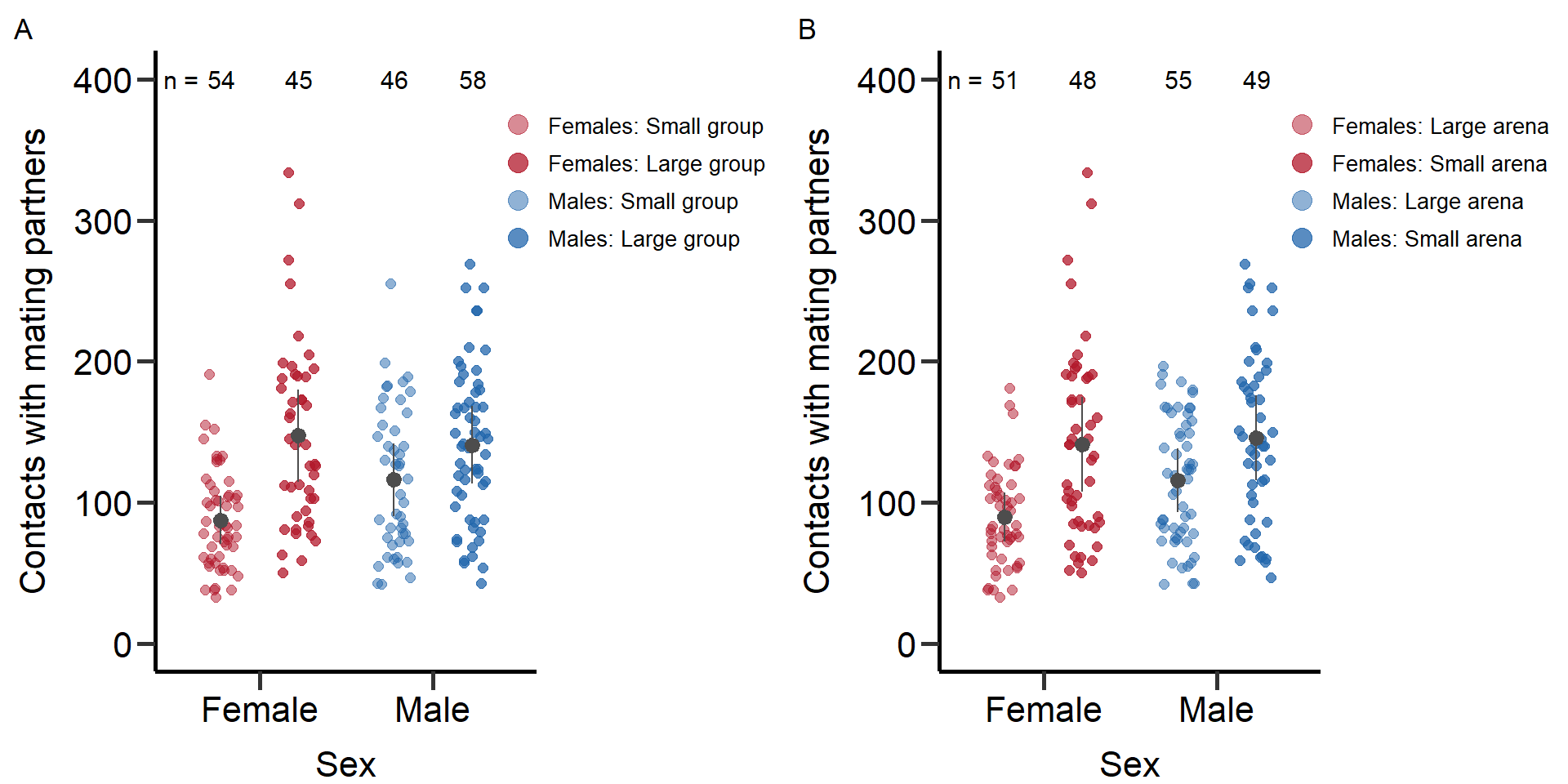
Figure S1: Total number of contacts with potential mating partners for males and females under low and high density manipulation via group (left) and arena size (right). Grey bars indicate means and standard deviations.
Figure_S1<-plot_grid(Figure_S1, ncol=1, rel_heights=c(0.1, 1))Bootstrapping the variance in contact rates
## Bootstrapping the variance in contact rates ####
# Male
# Large group size

D_data_Large_pop_M_Contact_n <-as.vector(D_data_Large_pop$N_contact_WT[D_data_Large_pop$Sex=='M'])
c <- function(d, i){
  d2 <- d[i]
  return(sd(d2, na.rm=TRUE)/mean(d2, na.rm=TRUE))
}
Large_pop_M_Contact_bootvar <- boot(D_data_Large_pop_M_Contact_n, c, R=10000)

# Small group size
D_data_Small_pop_M_Contact_n <-as.vector(D_data_Small_pop$N_contact_WT[D_data_Large_pop$Sex=='M'])

Small_pop_M_Contact_bootvar <- boot(D_data_Small_pop_M_Contact_n, c, R=10000)

# Large arena
D_data_Large_arena_M_Contact_n <-as.vector(D_data_Large_arena$N_contact_WT[D_data_Large_pop$Sex=='M'])

Large_arena_M_Contact_bootvar <- boot(D_data_Large_arena_M_Contact_n, c, R=10000)

# Small arena
D_data_Small_arena_M_Contact_n <-as.vector(D_data_Small_arena$N_contact_WT[D_data_Large_pop$Sex=='M'])

Small_arena_M_Contact_bootvar <- boot(D_data_Small_arena_M_Contact_n, c, R=10000)

# Female
# Large group size
D_data_Large_pop_F_Contact_n <-as.vector(D_data_Large_pop$N_contact_WT[D_data_Large_pop$Sex=='F'])

Large_pop_F_Contact_bootvar <- boot(D_data_Large_pop_F_Contact_n, c, R=10000)

# Small group size
D_data_Small_pop_F_Contact_n <-as.vector(D_data_Small_pop$N_contact_WT[D_data_Large_pop$Sex=='F'])

Small_pop_F_Contact_bootvar <- boot(D_data_Small_pop_F_Contact_n, c, R=10000)

# Large arena
D_data_Large_arena_F_Contact_n <-as.vector(D_data_Large_arena$N_contact_WT[D_data_Large_pop$Sex=='F'])

Large_arena_F_Contact_bootvar <- boot(D_data_Large_arena_F_Contact_n, c, R=10000)

# Small arena
D_data_Small_arena_F_Contact_n <-as.vector(D_data_Small_arena$N_contact_WT[D_data_Large_pop$Sex=='F'])

Small_arena_F_Contact_bootvar <- boot(D_data_Small_arena_F_Contact_n, c, R=10000)

# Extract data and write results table
PhenVarBoot_Table_Male_Small_pop_Contact <- as.data.frame(cbind("Male", "Small population size", "Contacts with pot. partners", as.numeric(mean(Small_pop_M_Contact_bootvar$t)), quantile(Small_pop_M_Contact_bootvar$t,.025, names = FALSE), quantile(Small_pop_M_Contact_bootvar$t,.975, names = FALSE)))
PhenVarBoot_Table_Male_Large_pop_Contact <- as.data.frame(cbind("Male", "Large population size", "Contacts with pot. partners", as.numeric(mean(Large_pop_M_Contact_bootvar$t)), quantile(Large_pop_M_Contact_bootvar$t,.025, names = FALSE), quantile(Large_pop_M_Contact_bootvar$t,.975, names = FALSE)))
PhenVarBoot_Table_Female_Small_pop_Contact <- as.data.frame(cbind("Female", "Small population size", "Contacts with pot. partners", as.numeric(mean(Small_pop_F_Contact_bootvar$t)), quantile(Small_pop_F_Contact_bootvar$t,.025, names = FALSE), quantile(Small_pop_F_Contact_bootvar$t,.975, names = FALSE)))
PhenVarBoot_Table_Female_Large_pop_Contact <- as.data.frame(cbind("Female", "Large population size", "Contacts with pot. partners", as.numeric(mean(Large_pop_F_Contact_bootvar$t)), quantile(Large_pop_F_Contact_bootvar$t,.025, names = FALSE), quantile(Large_pop_F_Contact_bootvar$t,.975, names = FALSE)))
PhenVarBoot_Table_Male_Small_arena_Contact <- as.data.frame(cbind("Male", "Small arena size", "Contacts with pot. partners", as.numeric(mean(Small_arena_M_Contact_bootvar$t)), quantile(Small_arena_M_Contact_bootvar$t,.025, names = FALSE), quantile(Small_arena_M_Contact_bootvar$t,.975, names = FALSE)))
PhenVarBoot_Table_Male_Large_arena_Contact <- as.data.frame(cbind("Male", "Large arena size", "Contacts with pot. partners", as.numeric(mean(Large_arena_M_Contact_bootvar$t)), quantile(Large_arena_M_Contact_bootvar$t,.025, names = FALSE), quantile(Large_arena_M_Contact_bootvar$t,.975, names = FALSE)))
PhenVarBoot_Table_Female_Small_arena_Contact <- as.data.frame(cbind("Female", "Small arena size", "Contacts with pot. partners", as.numeric(mean(Small_arena_F_Contact_bootvar$t)), quantile(Small_arena_F_Contact_bootvar$t,.025, names = FALSE), quantile(Small_arena_F_Contact_bootvar$t,.975, names = FALSE)))
PhenVarBoot_Table_Female_Large_arena_Contact <- as.data.frame(cbind("Female", "Large arena size", "Contacts with pot. partners", as.numeric(mean(Large_arena_F_Contact_bootvar$t)), quantile(Large_arena_F_Contact_bootvar$t,.025, names = FALSE), quantile(Large_arena_F_Contact_bootvar$t,.975, names = FALSE)))

Table_VarCont <- as.data.frame(as.matrix(rbind(PhenVarBoot_Table_Male_Small_pop_Contact,PhenVarBoot_Table_Male_Large_pop_Contact,
                                               PhenVarBoot_Table_Female_Small_pop_Contact,PhenVarBoot_Table_Female_Large_pop_Contact,
                                               PhenVarBoot_Table_Male_Small_arena_Contact,PhenVarBoot_Table_Male_Large_arena_Contact,
                                               PhenVarBoot_Table_Female_Small_arena_Contact,PhenVarBoot_Table_Female_Large_arena_Contact)),digits=3)

is.table(Table_VarCont)
colnames(Table_VarCont)[1] <- "Sex"
colnames(Table_VarCont)[2] <- "Treatment"
colnames(Table_VarCont)[3] <- "Trait"
colnames(Table_VarCont)[4] <- "Variance"
colnames(Table_VarCont)[5] <- "l95_CI"
colnames(Table_VarCont)[6] <- "u95_CI"
Table_VarCont[,4]=as.numeric(Table_VarCont[,4])
Table_VarCont[,5]=as.numeric(Table_VarCont[,5])
Table_VarCont[,6]=as.numeric(Table_VarCont[,6])

rm(c) # Remove bootstrapping functionkable(head(Table_VarCont))| Sex | Treatment | Trait | Variance | l95_CI | u95_CI |
|---|---|---|---|---|---|
| Male | Small population size | Contacts with pot. partners | 0.4354201 | 0.3745551 | 0.4960761 |
| Male | Large population size | Contacts with pot. partners | 0.3872321 | 0.3227348 | 0.4534341 |
| Female | Small population size | Contacts with pot. partners | 0.4437505 | 0.3577724 | 0.5337895 |
| Female | Large population size | Contacts with pot. partners | 0.4377419 | 0.3519710 | 0.5237236 |
| Male | Small arena size | Contacts with pot. partners | 0.5089506 | 0.4279041 | 0.5888735 |
| Male | Large arena size | Contacts with pot. partners | 0.4100654 | 0.3532523 | 0.4681418 |
Permutation test for treatment comparison of contact rates
## Permutation test for treatment comparison of contact rates ####
# Male
# Group size
Treat_diff_Male_pop_Contact=c(Large_pop_M_Contact_bootvar$t)-c(Small_pop_M_Contact_bootvar$t)

t_Treat_diff_Male_pop_Contact=mean(Treat_diff_Male_pop_Contact,na.rm=TRUE)
t_Treat_diff_Male_pop_Contact_lower=quantile(Treat_diff_Male_pop_Contact,.025,na.rm=TRUE)
t_Treat_diff_Male_pop_Contact_upper=quantile(Treat_diff_Male_pop_Contact,.975,na.rm=TRUE)

#Permutation test to calculate p value
comb_data=c(D_data_Large_pop$N_contact_WT[D_data_Large_pop$Sex=='M'],D_data_Small_pop$N_contact_WT[D_data_Small_pop$Sex=='M'])

diff.observed = sd(na.omit((D_data_Large_pop$N_contact_WT[D_data_Large_pop$Sex=='M'])))/mean(na.omit((D_data_Large_pop$N_contact_WT[D_data_Large_pop$Sex=='M'])))-sd(na.omit((D_data_Small_pop$N_contact_WT[D_data_Small_pop$Sex=='M'])))/mean(na.omit((D_data_Small_pop$N_contact_WT[D_data_Small_pop$Sex=='M'])))

number_of_permutations = 100000
diff.random = NULL
for (i in 1 : number_of_permutations) {

  # Sample from the combined data set
  a.random = sample (na.omit(comb_data), length(c(D_data_Large_pop$N_contact_WT[D_data_Large_pop$Sex=='M'])), TRUE)
  b.random = sample (na.omit(comb_data), length(c(D_data_Small_pop$N_contact_WT[D_data_Small_pop$Sex=='M'])), TRUE)

  # Null (permuated) difference
  diff.random[i] =  sd(na.omit(a.random))/mean(na.omit(a.random))-sd(na.omit(b.random))/mean(na.omit(b.random))
}

# P-value is the fraction of how many times the permuted difference is equal or more extreme than the observed difference

t_Treat_diff_Male_pop_Contact_p = sum(abs(diff.random) >= as.numeric(abs(diff.observed)))/   number_of_permutations

# Arena
Treat_diff_Male_arena_Contact=c(Small_arena_M_Contact_bootvar$t)-c(Large_arena_M_Contact_bootvar$t)

t_Treat_diff_Male_arena_Contact=mean(Treat_diff_Male_arena_Contact,na.rm=TRUE)
t_Treat_diff_Male_arena_Contact_lower=quantile(Treat_diff_Male_arena_Contact,.025,na.rm=TRUE)
t_Treat_diff_Male_arena_Contact_upper=quantile(Treat_diff_Male_arena_Contact,.975,na.rm=TRUE)

#Permutation test to calculate p value
comb_data=c(D_data_Large_arena$N_contact_WT[D_data_Large_arena$Sex=='M'],D_data_Small_arena$N_contact_WT[D_data_Small_arena$Sex=='M'])

diff.observed = sd(na.omit((D_data_Small_arena$N_contact_WT[D_data_Small_arena$Sex=='M'])))/mean(na.omit((D_data_Small_arena$N_contact_WT[D_data_Small_arena$Sex=='M'])))-sd(na.omit((D_data_Large_arena$N_contact_WT[D_data_Large_arena$Sex=='M'])))/mean(na.omit((D_data_Large_arena$N_contact_WT[D_data_Large_arena$Sex=='M'])))

number_of_permutations = 100000
diff.random = NULL
for (i in 1 : number_of_permutations) {

  # Sample from the combined data set
  b.random = sample (na.omit(comb_data), length(c(D_data_Large_arena$N_contact_WT[D_data_Large_arena$Sex=='M'])), TRUE)
  a.random = sample (na.omit(comb_data), length(c(D_data_Small_arena$N_contact_WT[D_data_Small_arena$Sex=='M'])), TRUE)

  # Null (permuated) difference
  diff.random[i] =  sd(na.omit(a.random))/mean(na.omit(a.random))-sd(na.omit(b.random))/mean(na.omit(b.random))
}

t_Treat_diff_Male_arena_Contact_p = sum(abs(diff.random) >= as.numeric(abs(diff.observed)))/   number_of_permutations

# Female
# Group size
Treat_diff_Female_pop_Contact=c(Large_pop_F_Contact_bootvar$t)-c(Small_pop_F_Contact_bootvar$t)

t_Treat_diff_Female_pop_Contact=mean(Treat_diff_Female_pop_Contact,na.rm=TRUE)
t_Treat_diff_Female_pop_Contact_lower=quantile(Treat_diff_Female_pop_Contact,.025,na.rm=TRUE)
t_Treat_diff_Female_pop_Contact_upper=quantile(Treat_diff_Female_pop_Contact,.975,na.rm=TRUE)

#Permutation test to calculate p value
comb_data=c(D_data_Large_pop$N_contact_WT[D_data_Large_pop$Sex=='F'],D_data_Small_pop$N_contact_WT[D_data_Small_pop$Sex=='F'])

diff.observed = sd(na.omit((D_data_Large_pop$N_contact_WT[D_data_Large_pop$Sex=='F'])))/mean(na.omit((D_data_Large_pop$N_contact_WT[D_data_Large_pop$Sex=='F'])))- sd(na.omit((D_data_Small_pop$N_contact_WT[D_data_Small_pop$Sex=='F'])))/mean(na.omit((D_data_Small_pop$N_contact_WT[D_data_Small_pop$Sex=='F'])))

number_of_permutations = 100000
diff.random = NULL
for (i in 1 : number_of_permutations) {

  # Sample from the combined data set
  a.random = sample (na.omit(comb_data), length(c(D_data_Large_pop$N_contact_WT[D_data_Large_pop$Sex=='F'])), TRUE)
  b.random = sample (na.omit(comb_data), length(c(D_data_Small_pop$N_contact_WT[D_data_Small_pop$Sex=='F'])), TRUE)

  # Null (permuated) difference
  diff.random[i] =  sd(na.omit(a.random))/mean(na.omit(a.random))-sd(na.omit(b.random))/mean(na.omit(b.random))
}

t_Treat_diff_Female_pop_Contact_p = sum(abs(diff.random) >= as.numeric(abs(diff.observed)))/   number_of_permutations

# Arena
Treat_diff_Female_arena_Contact=c(Small_arena_F_Contact_bootvar$t)-c(Large_arena_F_Contact_bootvar$t)

t_Treat_diff_Female_arena_Contact=mean(Treat_diff_Female_arena_Contact,na.rm=TRUE)
t_Treat_diff_Female_arena_Contact_lower=quantile(Treat_diff_Female_arena_Contact,.025,na.rm=TRUE)
t_Treat_diff_Female_arena_Contact_upper=quantile(Treat_diff_Female_arena_Contact,.975,na.rm=TRUE)

#Permutation test to calculate p value
comb_data=c(D_data_Large_arena$N_contact_WT[D_data_Large_arena$Sex=='F'],D_data_Small_arena$N_contact_WT[D_data_Small_arena$Sex=='F'])

diff.observed = sd(na.omit((D_data_Small_arena$N_contact_WT[D_data_Small_arena$Sex=='F'])))/mean(na.omit((D_data_Small_arena$N_contact_WT[D_data_Small_arena$Sex=='F'])))-sd(na.omit((D_data_Large_arena$N_contact_WT[D_data_Large_arena$Sex=='F'])))/mean(na.omit((D_data_Large_arena$N_contact_WT[D_data_Large_arena$Sex=='F'])))

number_of_permutations = 100000
diff.random = NULL
for (i in 1 : number_of_permutations) {

  # Sample from the combined data set
  b.random = sample (na.omit(comb_data), length(c(D_data_Large_arena$N_contact_WT[D_data_Large_arena$Sex=='F'])), TRUE)
  a.random = sample (na.omit(comb_data), length(c(D_data_Small_arena$N_contact_WT[D_data_Small_arena$Sex=='F'])), TRUE)

  # Null (permuated) difference
  diff.random[i] =  sd(na.omit(a.random))/mean(na.omit(a.random))-sd(na.omit(b.random))/mean(na.omit(b.random))
}

t_Treat_diff_Female_arena_Contact_p = sum(abs(diff.random) >= as.numeric(abs(diff.observed)))/   number_of_permutations

# Extract data and write data table
CompTreat_Table_Male_pop_Contact <- as.data.frame(cbind("Male", "Group size", "Contacts with pot. partners", t_Treat_diff_Male_pop_Contact, t_Treat_diff_Male_pop_Contact_lower, t_Treat_diff_Male_pop_Contact_upper, t_Treat_diff_Male_pop_Contact_p))
names(CompTreat_Table_Male_pop_Contact)=c('V1','V2','V3','V4','V5','V6','V7')
CompTreat_Table_Female_pop_Contact <- as.data.frame(cbind("Female", "Group size", "Contacts with pot. partners", t_Treat_diff_Female_pop_Contact, t_Treat_diff_Female_pop_Contact_lower, t_Treat_diff_Female_pop_Contact_upper, t_Treat_diff_Female_pop_Contact_p))
names(CompTreat_Table_Female_pop_Contact)=c('V1','V2','V3','V4','V5','V6','V7')
CompTreat_Table_Male_arena_Contact <- as.data.frame(cbind("Male", "Arena size", "Contacts with pot. partners", t_Treat_diff_Male_arena_Contact, t_Treat_diff_Male_arena_Contact_lower, t_Treat_diff_Male_arena_Contact_upper, t_Treat_diff_Male_arena_Contact_p))
names(CompTreat_Table_Male_arena_Contact)=c('V1','V2','V3','V4','V5','V6','V7')
CompTreat_Table_Female_arena_Contact <- as.data.frame(cbind("Female", "Arena size", "Contacts with pot. partners", t_Treat_diff_Female_arena_Contact, t_Treat_diff_Female_arena_Contact_lower, t_Treat_diff_Female_arena_Contact_upper, t_Treat_diff_Female_arena_Contact_p))
names(CompTreat_Table_Female_arena_Contact)=c('V1','V2','V3','V4','V5','V6','V7')

Table_varCont_TreatComp <- as.data.frame(as.matrix(rbind(CompTreat_Table_Male_pop_Contact,CompTreat_Table_Female_pop_Contact,
                                                         CompTreat_Table_Male_arena_Contact,CompTreat_Table_Female_arena_Contact)))

Table_varCont_TreatComp[,4]=as.numeric(Table_varCont_TreatComp[,4])
Table_varCont_TreatComp[,5]=as.numeric(Table_varCont_TreatComp[,5])
Table_varCont_TreatComp[,6]=as.numeric(Table_varCont_TreatComp[,6])
Table_varCont_TreatComp[,7]=as.numeric(Table_varCont_TreatComp[,7])

colnames(Table_varCont_TreatComp)[1] <- "Sex"
colnames(Table_varCont_TreatComp)[2] <- "Treatment"
colnames(Table_varCont_TreatComp)[3] <- "Trait"
colnames(Table_varCont_TreatComp)[4] <- "Variance"
colnames(Table_varCont_TreatComp)[5] <- "l95_CI"
colnames(Table_varCont_TreatComp)[6] <- "u95_CI"
colnames(Table_varCont_TreatComp)[7] <- "Adj. p-value"
Table_varCont_TreatComp[,7]=c(round(p.adjust(c(0.32852 ,0.61279   ), method = 'fdr'),digit=3),round(p.adjust(c(0.52590 ,0.24217    ), method = 'fdr'),digit=3))

Table_varCont_TreatComp[,4]=round(as.numeric(Table_varCont_TreatComp[,4]),digits=2)
Table_varCont_TreatComp[,5]=round(as.numeric(Table_varCont_TreatComp[,5]),digits=2)
Table_varCont_TreatComp[,6]=round(as.numeric(Table_varCont_TreatComp[,6]),digits=2)
Table_varCont_TreatComp[,7]=as.numeric(Table_varCont_TreatComp[,7])
rownames(Table_varCont_TreatComp) <- c()

round(p.adjust(c(0.32852 ,0.61279   ), method = 'fdr'),digit=3) # Calculate FDR adjusted p-values for males
round(p.adjust(c(0.52590 ,0.24217    ), method = 'fdr'),digit=3) # Calculate FDR adjusted p-values for females
#Table_varCont_TreatComp=as.table(Table_varCont_TreatComp,row.names=FALSE)
kable(head(Table_varCont_TreatComp))| Sex | Treatment | Trait | Variance | l95_CI | u95_CI | Adj. p-value |
|---|---|---|---|---|---|---|
| Male | Group size | Contacts with pot. partners | -0.05 | -0.14 | 0.04 | 0.613 |
| Female | Group size | Contacts with pot. partners | -0.01 | -0.13 | 0.12 | 0.613 |
| Male | Arena size | Contacts with pot. partners | 0.10 | 0.00 | 0.20 | 0.526 |
| Female | Arena size | Contacts with pot. partners | -0.06 | -0.16 | 0.04 | 0.484 |
sessionInfo()R version 4.2.0 (2022-04-22 ucrt)
Platform: x86_64-w64-mingw32/x64 (64-bit)
Running under: Windows 10 x64 (build 19045)
Matrix products: default
locale:
[1] LC_COLLATE=German_Germany.utf8 LC_CTYPE=German_Germany.utf8
[3] LC_MONETARY=German_Germany.utf8 LC_NUMERIC=C
[5] LC_TIME=German_Germany.utf8
attached base packages:
[1] grid stats graphics grDevices utils datasets methods
[8] base
other attached packages:
[1] knitr_1.42 ICC_2.4.0 data.table_1.14.8 boot_1.3-28
[5] RColorBrewer_1.1-3 car_3.1-1 carData_3.0-5 gridGraphics_0.5-1
[9] cowplot_1.1.1 EnvStats_2.7.0 dplyr_1.1.0 readr_2.1.4
[13] lmerTest_3.1-3 lme4_1.1-31 Matrix_1.5-3 gridExtra_2.3
[17] ggplot2_3.4.1 ggeffects_1.2.0
loaded via a namespace (and not attached):
[1] Rcpp_1.0.10 lattice_0.20-45 rprojroot_2.0.3
[4] digest_0.6.31 utf8_1.2.3 R6_2.5.1
[7] evaluate_0.20 highr_0.10 pillar_1.8.1
[10] rlang_1.0.6 rstudioapi_0.14 minqa_1.2.5
[13] whisker_0.4.1 jquerylib_0.1.4 nloptr_2.0.3
[16] rmarkdown_2.20 labeling_0.4.2 splines_4.2.0
[19] stringr_1.5.0 bit_4.0.5 munsell_0.5.0
[22] compiler_4.2.0 numDeriv_2016.8-1.1 httpuv_1.6.9
[25] xfun_0.37 pkgconfig_2.0.3 htmltools_0.5.4
[28] tidyselect_1.2.0 tibble_3.2.0 workflowr_1.7.0
[31] fansi_1.0.4 crayon_1.5.2 tzdb_0.3.0
[34] withr_2.5.0 later_1.3.0 MASS_7.3-56
[37] nlme_3.1-157 jsonlite_1.8.4 gtable_0.3.1
[40] lifecycle_1.0.3 git2r_0.31.0 magrittr_2.0.3
[43] scales_1.2.1 vroom_1.6.1 cli_3.6.1
[46] stringi_1.7.12 cachem_1.0.7 farver_2.1.1
[49] fs_1.6.1 promises_1.2.0.1 bslib_0.4.2
[52] ellipsis_0.3.2 generics_0.1.3 vctrs_0.5.2
[55] tools_4.2.0 bit64_4.0.5 glue_1.6.2
[58] hms_1.1.2 parallel_4.2.0 abind_1.4-5
[61] fastmap_1.1.1 yaml_2.3.7 colorspace_2.1-0
[64] sass_0.4.5