Stronger net selection on males across animals
Supplementary material reporting R code
Lennart Winkler1, Maria Moiron2, Edward H. Morrow3 and Tim Janicke1,2
1Applied Zoology, Technical University Dresden
2Centre d’Écologie Fonctionnelle et Évolutive, UMR 5175, CNRS, Université de Montpellier 3Department for Environmental and Life Sciences, Karlstad University
Last updated: 2021-06-23
Checks: 7 0
Knit directory: Net_Selection_eLife_code/
This reproducible R Markdown analysis was created with workflowr (version 1.6.2). The Checks tab describes the reproducibility checks that were applied when the results were created. The Past versions tab lists the development history.
Great! Since the R Markdown file has been committed to the Git repository, you know the exact version of the code that produced these results.
Great job! The global environment was empty. Objects defined in the global environment can affect the analysis in your R Markdown file in unknown ways. For reproduciblity it’s best to always run the code in an empty environment.
The command set.seed(20210613) was run prior to running the code in the R Markdown file. Setting a seed ensures that any results that rely on randomness, e.g. subsampling or permutations, are reproducible.
Great job! Recording the operating system, R version, and package versions is critical for reproducibility.
Nice! There were no cached chunks for this analysis, so you can be confident that you successfully produced the results during this run.
Great job! Using relative paths to the files within your workflowr project makes it easier to run your code on other machines.
Great! You are using Git for version control. Tracking code development and connecting the code version to the results is critical for reproducibility.
The results in this page were generated with repository version f7593bd. See the Past versions tab to see a history of the changes made to the R Markdown and HTML files.
Note that you need to be careful to ensure that all relevant files for the analysis have been committed to Git prior to generating the results (you can use wflow_publish or wflow_git_commit). workflowr only checks the R Markdown file, but you know if there are other scripts or data files that it depends on. Below is the status of the Git repository when the results were generated:
Ignored files:
    Ignored:    .Rhistory
    Ignored:    data/.Rhistory

Untracked files:
    Untracked:  analysis/docs/.nojekyll
    Untracked:  analysis/docs/about.html
    Untracked:  analysis/docs/license.html
    Untracked:  analysis/docs/site_libs/
    Untracked:  data/META_SexSpecGenVar_Data_v23.csv
    Untracked:  data/META_SexSpecGenVar_Pylogeny_v05_NEWICK.txt
Note that any generated files, e.g. HTML, png, CSS, etc., are not included in this status report because it is ok for generated content to have uncommitted changes.
These are the previous versions of the repository in which changes were made to the R Markdown (analysis/index.Rmd) and HTML (docs/index.html) files. If you’ve configured a remote Git repository (see ?wflow_git_remote), click on the hyperlinks in the table below to view the files as they were in that past version.
| File | Version | Author | Date | Message |
|---|---|---|---|---|
| Rmd | f7593bd | LennartWinkler | 2021-06-23 | wflow_publish(all = T) |
| html | f7593bd | LennartWinkler | 2021-06-23 | wflow_publish(all = T) |
| html | 98c553d | LennartWinkler | 2021-06-23 | Build site. |
| Rmd | 926ceb8 | LennartWinkler | 2021-06-23 | wflow_publish(all = T) |
| html | 926ceb8 | LennartWinkler | 2021-06-23 | wflow_publish(all = T) |
| html | 3bccaab | LennartWinkler | 2021-06-23 | Build site. |
| Rmd | 7ffcf00 | LennartWinkler | 2021-06-23 | wflow_publish(all = T) |
| html | 7ffcf00 | LennartWinkler | 2021-06-23 | wflow_publish(all = T) |
| html | 63df934 | LennartWinkler | 2021-06-23 | Build site. |
| Rmd | 36c6fdc | LennartWinkler | 2021-06-23 | wflow_publish(all = T) |
| html | 36c6fdc | LennartWinkler | 2021-06-23 | wflow_publish(all = T) |
| html | b3577de | LennartWinkler | 2021-06-23 | Build site. |
| Rmd | 85c0b6e | LennartWinkler | 2021-06-23 | wflow_publish(all = T) |
| html | 85c0b6e | LennartWinkler | 2021-06-23 | wflow_publish(all = T) |
| html | 4ed93cf | LennartWinkler | 2021-06-23 | Build site. |
| Rmd | 058af7b | LennartWinkler | 2021-06-23 | wflow_publish(all = T) |
| html | 058af7b | LennartWinkler | 2021-06-23 | wflow_publish(all = T) |
| html | 223df21 | LennartWinkler | 2021-06-23 | Build site. |
| Rmd | f63b665 | LennartWinkler | 2021-06-23 | wflow_publish(all = T) |
| html | f63b665 | LennartWinkler | 2021-06-23 | wflow_publish(all = T) |
| html | 3139eb4 | LennartWinkler | 2021-06-14 | Build site. |
| Rmd | 9290105 | LennartWinkler | 2021-06-14 | wflow_publish(all = TRUE) |
| html | 9290105 | LennartWinkler | 2021-06-14 | wflow_publish(all = TRUE) |
| html | 01525f8 | LennartWinkler | 2021-06-13 | Build site. |
| Rmd | 161eee9 | LennartWinkler | 2021-06-13 | wflow_publish(“C:/Users/lenna/Desktop/Documents/PhD/2020_META SexSpecGenVar/eLife/Net_Selection_eLife_code/analysis/index.Rmd”) |
| html | 6f60c27 | LennartWinkler | 2021-06-13 | Build site. |
| Rmd | 555a290 | LennartWinkler | 2021-06-13 | wflow_publish(“C:/Users/lenna/Documents/Net_Selection_eLife_code/analysis/index.Rmd”) |
| html | 9220292 | LennartWinkler | 2021-06-13 | Build site. |
| Rmd | 15f14fe | LennartWinkler | 2021-06-13 | wflow_publish(“C:/Users/lenna/Documents/Net_Selection_eLife_code/analysis/index.Rmd”) |
| html | db2f16f | LennartWinkler | 2021-06-13 | Build site. |
| Rmd | 00738af | LennartWinkler | 2021-06-13 | wflow_publish(“C:/Users/lenna/Documents/Net_Selection_eLife_code/analysis/index.Rmd”) |
| html | 7d5ef2c | LennartWinkler | 2021-06-13 | Build site. |
| Rmd | 320011b | LennartWinkler | 2021-06-13 | Start workflowr project. |
Supplementary material reporting R code for the manuscript ‘Stronger net selection on males across animals’.
Phenotypic gambit
Statistical analyses were carried out in two steps. First, we examined the key assumption of the ‘phenotypic gambit’ by testing whether estimates of phenotypic variance predict the estimated genetic variance. For this we computed the Pearson correlation coefficient r, testing the relationship between CVP and CVG for both sexes and the two fitness components separately. In addition, we tested whether the sex bias in CVP translates into a sex bias in CVG by correlating the coefficient of variation ratio lnCVR (Nakagawa et al. 2015), which refers to the ln-transformed ratio of male CV to female CV, with positive values indicating a male bias. The analyses on the phenotypic gambit were motivated from a methodological perspective and we did not expect that inter-specific variation in the difference between CVP and CVG can be explained by a shared phylogenetic history. However, for completeness, we also ran correlations on phylogenetic independent contrasts (PICs; computed using the ape R-package (version 5.4.1) in R (Paradis & Schliep 2019)) to test whether our findings were robust when accounting for potential phylogenetic non-independence. We report Pearson’s correlation coefficients r for normally distributed data and Spearman’s rho if assumptions of normality were violated.
Load and prepare data
Stronger net selection on males (PGLMMs)
In this second part of the anlysis, we tested the hypothesis that net selection is stronger on males by testing for a male bias in CVP and CVG. Specifically, we ran Phylogenetic General Linear Mixed-Effects Models (PGLMMs) with CVP or CVG as the response variable, and sex as a fixed effect. To account for the paired data structure, we added an observation identifier as a random effect. Moreover, all models included a study identifier and the phylogeny (transformed into a correlation matrix) as random effects to account for statistical non-independence arising from shared study design or phylogenetic history, respectively. Note that the latter also accounts for the non-independence of estimates obtained from the same species as some studies estimated genetic variances from distinct field populations (Fox et al. 2004) or different experimental treatments under laboratory conditions such as food stress (Holman & Jacomb 2017) and temperature stress (Berger et al. 2014). In an additional series of PGLMMs we tested whether our proxy of sexual selection explained inter-specific variation in the sex-differences of CVP or CVG by adding mating system and its interaction with sex as fixed effects to the models. Finally, given that primary studies varied in the empirical approach used to quantify CVP and CVG, we also used PGLMMs to test whether study type (23 field studies versus 32 laboratory studies) represented a methodological determinant of the observed sex-differences in CVP and CVG. All PGLMMs were ran with the MCMCglmm R-package (version 2.2.9) (Hadfield 2010), using uninformative priors (V = 1, nu = 0.002) and an effective sample size of 20000 (number of iterations = 11000000, burn-in = 1000000, thinning interval = 500). We computed the proportion of variance explained by fixed factors (‘marginal R2’) (Nakagawa & Schielzeth 2013). In addition, we quantified the phylogenetic signal as the phylogenetic heritability H2 (i.e., proportional variance in CVP or CVG explained by species identity), which is equivalent to Pagel’s 𝜆 (de Villemereuil & Nakagawa 2014). In a previous study testing for sex-specific phenotypic variances in reproductive success (Janicke et al. 2016), we ran formal meta-analyses using lnCVR as the tested effect size (Nakagawa et al. 2015). This is potentially a more powerful approach for comparing phenotypic variances but rendered unsuitable when comparing genetic variances. This is because the computation of the sampling variance of lnCVR is a function of the sample size of the sampled population and the point estimate of lnCVR (Nakagawa et al. 2015). However, genetic variances are estimates from statistical models and notorious for being estimated with low precision (i.e. have large confidence intervals). Therefore, using a meta-analytic approach for genetic variances using lnCVR as an effect size leads to overconfident estimation of the global effect size and is therefore likely to result in type-II-errors. However, to allow comparison with the previous meta-analysis, we report the outcome of phylogenetic meta-analyses on phenotypic variances using lnCVR in the Supplementary Material (Table S2), which largely reflects the results on the point estimates of CVP from PGLMMs.
Load and prepare data
We first load all neccessary packages.
# load packages
rm(list = ls())
library(ape);library(metafor); library(Matrix); library(MASS); library(pwr);library(multcomp);library(psych);library(outliers)
library(matrixcalc)
library(PerformanceAnalytics)
library(tidyr)
library(MCMCglmm)
library(matrixcalc)
library(dplyr)
library(stargazer)
library(data.table)
library(ggplot2)
library(readr)
We then load the data set (‘Data’) and the phylogenetic tree (‘theTree’).
# load data
Data <- read.csv("./data/META_SexSpecGenVar_Data_v23.csv", sep=",", header=TRUE,fileEncoding="UTF-8-BOM")
theTree <- read.tree("./data/META_SexSpecGenVar_Pylogeny_v05_NEWICK.txt")
Finally, we subset our data set for the analyses into the fitness categories (‘FitnessCat’) lifespan (‘LS’) and reproductive success (‘RS’).
## Reorganising and subsetting dataset ####

stacked_gen_Data <- gather(Data, key = "Sex",value = "genCV", genCV_male, genCV_female)
stacked_phen_Data <- gather(Data, key = "Sex",value = "phenCV", phenCV_male, phenCV_female)

RS_gen_metaData<-subset(stacked_gen_Data, FitnessCat == "RS")
LS_gen_metaData<-subset(stacked_gen_Data, FitnessCat == "LS")

RS_phen_metaData<-subset(stacked_phen_Data, FitnessCat == "RS")
LS_phen_metaData<-subset(stacked_phen_Data, FitnessCat == "LS")
Run MCMC models
We then ran MCMC models to test for differences in the phenotypic and genetic variances in males and females for the fitness categories reproductive success and lifespan.
First we prune the phylogenetic tree to the data subset.
## PRUNE PHYLOGENETIC TREE TO DATA SUBSET
RS_gen_metaData$animal <- factor(RS_gen_metaData$animal)
is.factor(RS_gen_metaData$animal)
RS_Species_Data <- unique(RS_gen_metaData$animal)
summary(RS_Species_Data)
RS_theTree<-drop.tip(theTree, theTree$tip.label[-na.omit(match(RS_Species_Data, theTree$tip.label))])
plot(RS_theTree)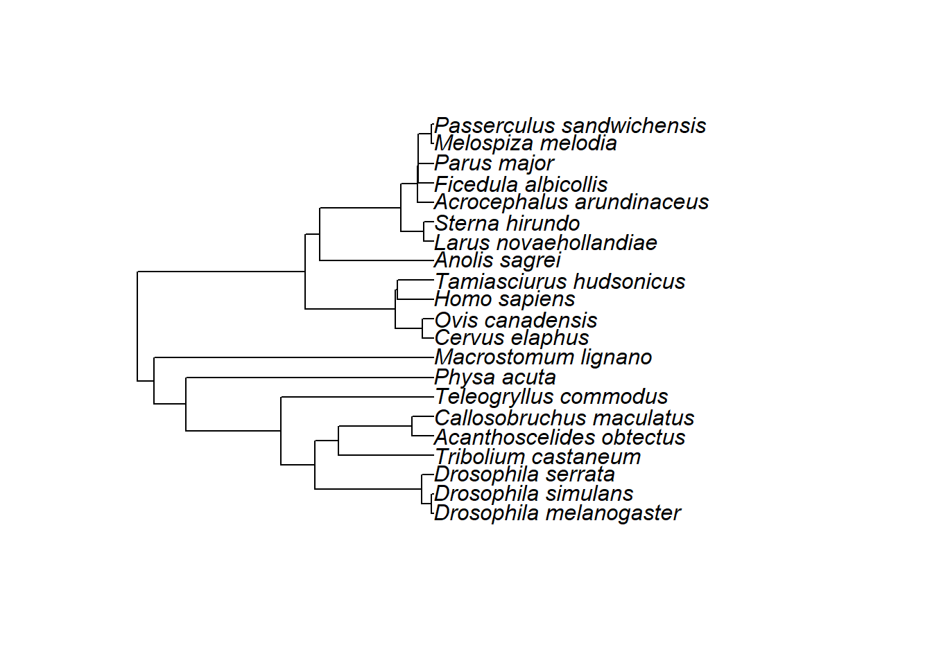
We then check if the phylogenetic tree was correctly build.
## CHECK PHYLOGENETIC TREE
sort(RS_theTree$tip.label) == sort(unique(RS_gen_metaData$animal)) # check if tip names correspond to data names
is.ultrametric(RS_theTree) # check if BL are aligned contemporaneously
isSymmetric(vcv(RS_theTree, corr=TRUE)) # check symmetry of phylogenetic correlation matrix
rawC <- vcv(RS_theTree, corr=TRUE)
is.positive.definite(rawC) # if FALSE will have to force symmetry
forcedC <- as.matrix(forceSymmetric(vcv(RS_theTree, corr=TRUE)))
is.positive.definite(forcedC)
comparedC <- rawC == forcedC
rawC[cbind(which(comparedC!=TRUE, arr.ind = T))] - forcedC[cbind(which(comparedC!=TRUE, arr.ind = T))] < 1e-5
Next, we set the priors for the MCMC models using uninformative priors (V = 1, nu = 0.002) and an effective sample size of 20000 (number of iterations = 11000000, burn-in = 1000000, thinning interval = 500). We also set the index and study ID as factors.
## Prior settings, iterations
pr<-list(R=list(V=1,nu=0.002), G=list(G1=list(V=1,nu=0.002),
                                      G2=list(V=1,nu=0.002),
                                      G3=list(V=1,nu=0.002)))

BURNIN = 100000
NITT   = 1100000
THIN   = 500

BURNIN = 10000
NITT   = 110000
THIN   = 500

RS_phen_metaData$Index <- as.factor(RS_phen_metaData$Index)
RS_phen_metaData$Study_ID <- as.factor(RS_phen_metaData$Study_ID)
RS_gen_metaData$Index <- as.factor(RS_gen_metaData$Index)
RS_gen_metaData$Study_ID <- as.factor(RS_gen_metaData$Study_ID)
MCMC models for reproductive success
First, we ran the MCMC testing for overall differences in phenotypic variance in reproductive success (‘phenCV’) between males and females (‘Sex’). The model includes the species (‘animal’), estimate ID (‘Index’) and study ID (‘Study_ID’) as random factors.
RS_phen_MCMC_model <- MCMCglmm(phenCV~factor(Sex),random=~animal + Index + Study_ID,
                          pedigree=RS_theTree,
                          prior=pr,
                          data=RS_phen_metaData,
                          pr = TRUE,
                          burnin = BURNIN,
                          nitt=NITT,
                          thin=THIN)

summary(RS_phen_MCMC_model)
 Iterations = 10001:109501
 Thinning interval  = 500
 Sample size  = 200

 DIC: 50.08103

 G-structure:  ~animal

       post.mean  l-95% CI u-95% CI eff.samp
animal    0.0215 0.0004836  0.08548      200

               ~Index

      post.mean l-95% CI u-95% CI eff.samp
Index   0.05882 0.001148   0.1242    267.8

               ~Study_ID

         post.mean l-95% CI u-95% CI eff.samp
Study_ID   0.06306 0.000233   0.1526    200.3

 R-structure:  ~units

      post.mean l-95% CI u-95% CI eff.samp
units   0.06034  0.03996  0.08267    117.8

 Location effects: phenCV ~ factor(Sex)

                       post.mean l-95% CI u-95% CI eff.samp  pMCMC
(Intercept)               0.6897   0.5147   0.9442      200 <0.005 **
factor(Sex)phenCV_male    0.2316   0.1426   0.2996      200 <0.005 **
---
Signif. codes:  0 '***' 0.001 '**' 0.01 '*' 0.05 '.' 0.1 ' ' 1
We then expanded the model to include the matingsytem as a covariate (‘Mating_system’).
RS_phen_MatSyst_MCMC_model <- MCMCglmm(phenCV~factor(Sex) * factor(Mating_system),random=~animal + Index + Study_ID,
                                  pedigree=RS_theTree,
                                  prior=pr,
                                  data=RS_phen_metaData,
                                  burnin = BURNIN,
                                  nitt=NITT,
                                  thin=THIN)

summary(RS_phen_MatSyst_MCMC_model)
 Iterations = 10001:109501
 Thinning interval  = 500
 Sample size  = 200

 DIC: 31.00689

 G-structure:  ~animal

       post.mean  l-95% CI u-95% CI eff.samp
animal    0.0415 0.0009463   0.1245      200

               ~Index

      post.mean  l-95% CI u-95% CI eff.samp
Index   0.06553 0.0006622   0.1327    345.3

               ~Study_ID

         post.mean  l-95% CI u-95% CI eff.samp
Study_ID   0.05893 0.0002484   0.1553      139

 R-structure:  ~units

      post.mean l-95% CI u-95% CI eff.samp
units   0.05102   0.0327   0.0685      200

 Location effects: phenCV ~ factor(Sex) * factor(Mating_system)

                                                     post.mean  l-95% CI
(Intercept)                                           0.705011  0.331216
factor(Sex)phenCV_male                               -0.008772 -0.203472
factor(Mating_system)polygamy                         0.008150 -0.297388
factor(Sex)phenCV_male:factor(Mating_system)polygamy  0.319035  0.120912
                                                      u-95% CI eff.samp  pMCMC
(Intercept)                                           1.091192      200   0.01
factor(Sex)phenCV_male                                0.136592      200   0.94
factor(Mating_system)polygamy                         0.489325      200   0.98
factor(Sex)phenCV_male:factor(Mating_system)polygamy  0.483260      200 <0.005

(Intercept)                                          *
factor(Sex)phenCV_male
factor(Mating_system)polygamy
factor(Sex)phenCV_male:factor(Mating_system)polygamy **
---
Signif. codes:  0 '***' 0.001 '**' 0.01 '*' 0.05 '.' 0.1 ' ' 1
In an additional model, we included the study type (‘StudyType’), i.e. if the data were obtained in laboratory or field experiments.
RS_phen_StudyType_MCMC_model <- MCMCglmm(phenCV~factor(Sex) * factor(StudyType),random=~animal + Index + Study_ID,
                                        pedigree=RS_theTree,
                                        prior=pr,
                                        data=RS_phen_metaData,
                                        burnin = BURNIN,
                                        nitt=NITT,
                                        thin=THIN)
summary(RS_phen_StudyType_MCMC_model)
 Iterations = 10001:109501
 Thinning interval  = 500
 Sample size  = 200

 DIC: 51.0445

 G-structure:  ~animal

       post.mean  l-95% CI u-95% CI eff.samp
animal   0.01296 0.0002984  0.04841      200

               ~Index

      post.mean l-95% CI u-95% CI eff.samp
Index   0.06457 0.005559   0.1166    228.2

               ~Study_ID

         post.mean  l-95% CI u-95% CI eff.samp
Study_ID   0.04607 0.0004687   0.1219      200

 R-structure:  ~units

      post.mean l-95% CI u-95% CI eff.samp
units   0.05913  0.03754  0.08295      200

 Location effects: phenCV ~ factor(Sex) * factor(StudyType)

                                                   post.mean l-95% CI u-95% CI
(Intercept)                                          0.88229  0.69786  1.13647
factor(Sex)phenCV_male                               0.19596  0.07779  0.32654
factor(StudyType)Laboratory                         -0.32085 -0.60583 -0.04419
factor(Sex)phenCV_male:factor(StudyType)Laboratory   0.06189 -0.11074  0.21244
                                                   eff.samp  pMCMC
(Intercept)                                           215.5 <0.005 **
factor(Sex)phenCV_male                                200.0   0.01 *
factor(StudyType)Laboratory                           200.0   0.03 *
factor(Sex)phenCV_male:factor(StudyType)Laboratory    200.0   0.45
---
Signif. codes:  0 '***' 0.001 '**' 0.01 '*' 0.05 '.' 0.1 ' ' 1
Next, we ran the MCMC models examining the genetic variance in reproductive success (‘genCV’). First, the overall model for a sex difference.
RS_gen_MCMC_model <- MCMCglmm(genCV~factor(Sex),random=~animal + Index + Study_ID,
                       pedigree=RS_theTree,
                       prior=pr,
                       data=RS_gen_metaData,
                       pr = TRUE,
                       burnin = BURNIN,
                       nitt=NITT,
                       thin=THIN)
summary(RS_gen_MCMC_model)
 Iterations = 10001:109501
 Thinning interval  = 500
 Sample size  = 200

 DIC: -130.0802

 G-structure:  ~animal

       post.mean  l-95% CI u-95% CI eff.samp
animal   0.01198 0.0004535  0.04331      200

               ~Index

      post.mean  l-95% CI u-95% CI eff.samp
Index  0.003847 0.0003005 0.009868      200

               ~Study_ID

         post.mean l-95% CI u-95% CI eff.samp
Study_ID   0.01471 0.004494  0.02548    248.7

 R-structure:  ~units

      post.mean l-95% CI u-95% CI eff.samp
units   0.01497 0.009596  0.02006      200

 Location effects: genCV ~ factor(Sex)

                      post.mean l-95% CI u-95% CI eff.samp  pMCMC
(Intercept)             0.24615  0.13462  0.37596    200.0 <0.005 **
factor(Sex)genCV_male   0.08424  0.04133  0.12205    149.8 <0.005 **
---
Signif. codes:  0 '***' 0.001 '**' 0.01 '*' 0.05 '.' 0.1 ' ' 1
Secondly, including the matingsytem as a covariate (‘Mating_system’).
RS_gen_MatSyst_MCMC_model <- MCMCglmm(genCV~factor(Sex) * factor(Mating_system),random=~animal + Index + Study_ID,
                  pedigree=RS_theTree,
                  prior=pr,
                  data=RS_gen_metaData,
                  burnin = BURNIN,
                  nitt=NITT,
                  thin=THIN)
summary(RS_gen_MatSyst_MCMC_model)
 Iterations = 10001:109501
 Thinning interval  = 500
 Sample size  = 200

 DIC: -138.7594

 G-structure:  ~animal

       post.mean  l-95% CI u-95% CI eff.samp
animal   0.01056 0.0002717  0.03152      200

               ~Index

      post.mean  l-95% CI u-95% CI eff.samp
Index  0.004712 0.0004249  0.01062      200

               ~Study_ID

         post.mean l-95% CI u-95% CI eff.samp
Study_ID   0.01545 0.005762  0.03144    156.5

 R-structure:  ~units

      post.mean l-95% CI u-95% CI eff.samp
units   0.01356 0.009133  0.01777      200

 Location effects: genCV ~ factor(Sex) * factor(Mating_system)

                                                    post.mean  l-95% CI
(Intercept)                                          0.254980  0.103623
factor(Sex)genCV_male                               -0.015821 -0.088028
factor(Mating_system)polygamy                       -0.007049 -0.146419
factor(Sex)genCV_male:factor(Mating_system)polygamy  0.135581  0.032283
                                                     u-95% CI eff.samp  pMCMC
(Intercept)                                          0.455024    200.0 <0.005
factor(Sex)genCV_male                                0.071933    200.0   0.74
factor(Mating_system)polygamy                        0.143565    272.4   0.98
factor(Sex)genCV_male:factor(Mating_system)polygamy  0.232928    246.3 <0.005

(Intercept)                                         **
factor(Sex)genCV_male
factor(Mating_system)polygamy
factor(Sex)genCV_male:factor(Mating_system)polygamy **
---
Signif. codes:  0 '***' 0.001 '**' 0.01 '*' 0.05 '.' 0.1 ' ' 1
And finally, we included the study type (‘StudyType’), i.e. if the data were obtained in laboratory or field experiments.
RS_gen_StudyType_MCMC_model <- MCMCglmm(genCV~factor(Sex) * factor(StudyType),random=~animal + Index + Study_ID,
                                      pedigree=RS_theTree,
                                      prior=pr,
                                      data=RS_gen_metaData,
                                      burnin = BURNIN,
                                      nitt=NITT,
                                      thin=THIN)
summary(RS_gen_StudyType_MCMC_model)
 Iterations = 10001:109501
 Thinning interval  = 500
 Sample size  = 200

 DIC: -127.4064

 G-structure:  ~animal

       post.mean  l-95% CI u-95% CI eff.samp
animal   0.01346 0.0004328  0.03499      200

               ~Index

      post.mean  l-95% CI u-95% CI eff.samp
Index  0.003754 0.0003163  0.00981    142.8

               ~Study_ID

         post.mean l-95% CI u-95% CI eff.samp
Study_ID    0.0143 0.003386   0.0273      200

 R-structure:  ~units

      post.mean l-95% CI u-95% CI eff.samp
units   0.01555  0.01059  0.02143      200

 Location effects: genCV ~ factor(Sex) * factor(StudyType)

                                                  post.mean  l-95% CI  u-95% CI
(Intercept)                                        0.171715 -0.088682  0.386666
factor(Sex)genCV_male                              0.080874  0.023493  0.161411
factor(StudyType)Laboratory                        0.127308 -0.071792  0.395470
factor(Sex)genCV_male:factor(StudyType)Laboratory  0.002628 -0.074388  0.084146
                                                  eff.samp pMCMC
(Intercept)                                          142.8  0.11
factor(Sex)genCV_male                                258.0  0.04 *
factor(StudyType)Laboratory                          129.2  0.27
factor(Sex)genCV_male:factor(StudyType)Laboratory    246.0  0.95
---
Signif. codes:  0 '***' 0.001 '**' 0.01 '*' 0.05 '.' 0.1 ' ' 1
R version 4.0.0 (2020-04-24)
Platform: x86_64-w64-mingw32/x64 (64-bit)
Running under: Windows 10 x64 (build 19041)

Matrix products: default

locale:
[1] LC_COLLATE=German_Germany.1252  LC_CTYPE=German_Germany.1252
[3] LC_MONETARY=German_Germany.1252 LC_NUMERIC=C
[5] LC_TIME=German_Germany.1252

attached base packages:
[1] stats     graphics  grDevices utils     datasets  methods   base

other attached packages:
 [1] readr_1.4.0                ggplot2_3.3.3
 [3] data.table_1.14.0          stargazer_5.2.2
 [5] dplyr_1.0.5                MCMCglmm_2.32
 [7] coda_0.19-4                tidyr_1.1.3
 [9] PerformanceAnalytics_2.0.4 xts_0.12.1
[11] zoo_1.8-9                  matrixcalc_1.0-3
[13] outliers_0.14              psych_2.1.3
[15] multcomp_1.4-16            TH.data_1.0-10
[17] survival_3.1-12            mvtnorm_1.1-1
[19] pwr_1.3-0                  MASS_7.3-51.5
[21] metafor_2.4-0              Matrix_1.2-18
[23] ape_5.4-1                  workflowr_1.6.2

loaded via a namespace (and not attached):
 [1] Rcpp_1.0.6        lattice_0.20-41   corpcor_1.6.9     assertthat_0.2.1
 [5] rprojroot_2.0.2   digest_0.6.27     utf8_1.2.1        R6_2.5.0
 [9] evaluate_0.14     highr_0.8         pillar_1.5.1      rlang_0.4.10
[13] cubature_2.0.4.1  whisker_0.4       rmarkdown_2.7     splines_4.0.0
[17] stringr_1.4.0     munsell_0.5.0     compiler_4.0.0    httpuv_1.6.1
[21] xfun_0.22         pkgconfig_2.0.3   mnormt_2.0.2      tmvnsim_1.0-2
[25] htmltools_0.5.1.1 tidyselect_1.1.0  tibble_3.1.0      tensorA_0.36.2
[29] quadprog_1.5-8    codetools_0.2-16  fansi_0.4.2       withr_2.4.1
[33] crayon_1.4.1      later_1.2.0       grid_4.0.0        gtable_0.3.0
[37] nlme_3.1-147      lifecycle_1.0.0   DBI_1.1.1         git2r_0.28.0
[41] magrittr_2.0.1    scales_1.1.1      stringi_1.5.3     fs_1.5.0
[45] promises_1.2.0.1  ellipsis_0.3.1    vctrs_0.3.6       generics_0.1.0
[49] sandwich_3.0-0    tools_4.0.0       glue_1.4.2        purrr_0.3.4
[53] hms_1.0.0         parallel_4.0.0    yaml_2.2.1        colorspace_2.0-0
[57] knitr_1.31