Global model Version 1

Global models Version 2

Moderator tests for phylogenetic models

Sexual selection mode
Plot sexual selection mode (Figure 2)
Sexual selection category
Plot sexual selection category (Figure S1)
Type of SSD measure
Plot Type of SSD measure (Figure S2A)
SSD measure controlled for body size?
Plot: SSD measure controlled for body size? (Figure S2B)
Phylogentic vs non-phylogenetic studies
Plot Phylogentic vs non-phylogenetic studies (Figure S2C)
Test for publication bias
Figure S2D
Publication year
Plot publication year (Figure S2E)

Moderator tests for non-phylogenetic models

Sexual selection mode
Sexual selection category
Phylogenetic classes
Plot phylogenetic classes (Figure 3)
Type of SSD measure
SSD measure controlled for body size?
Phylogentic vs non-phylogenetic studies
Test for publication bias
Publication year

Forest plot

Figure 1

Sexual selection and sexual size dimorphism: a meta-analysis of comparative studies

Main analyses

Lennart Winkler¹, Robert P Freckleton², Tamas Szekely³, ⁴ & Tim Janicke^1,5

¹Applied Zoology, Technical University Dresden

²Department of Zoology, University of Oxford, South Parks Road, Oxford OX1 3PS, UK

³Milner Centre for Evolution, University of Bath, Bath, UK8

⁴Department of Evolutionary Zoology and Human Behaviour, University of Debrecen, Debrecen, Hungary

⁵Centre d’Écologie Fonctionnelle et Évolutive, UMR 5175, CNRS, Université de Montpellier

Last updated: 2023-05-24

Checks: 7 0

Knit directory: SSD_and_sexual_selection_2023/

This reproducible R Markdown analysis was created with workflowr (version 1.7.0). The Checks tab describes the reproducibility checks that were applied when the results were created. The Past versions tab lists the development history.

R Markdown file: up-to-date

Great! Since the R Markdown file has been committed to the Git repository, you know the exact version of the code that produced these results.

Environment: empty

Great job! The global environment was empty. Objects defined in the global environment can affect the analysis in your R Markdown file in unknown ways. For reproduciblity it’s best to always run the code in an empty environment.

Seed: set.seed(20230430)

The command set.seed(20230430) was run prior to running the code in the R Markdown file. Setting a seed ensures that any results that rely on randomness, e.g. subsampling or permutations, are reproducible.

Session information: recorded

Great job! Recording the operating system, R version, and package versions is critical for reproducibility.

Cache: none

Nice! There were no cached chunks for this analysis, so you can be confident that you successfully produced the results during this run.

File paths: relative

Great job! Using relative paths to the files within your workflowr project makes it easier to run your code on other machines.

Repository version: c1d3311

Great! You are using Git for version control. Tracking code development and connecting the code version to the results is critical for reproducibility.

The results in this page were generated with repository version c1d3311. See the Past versions tab to see a history of the changes made to the R Markdown and HTML files.

Note that you need to be careful to ensure that all relevant files for the analysis have been committed to Git prior to generating the results (you can use wflow_publish or wflow_git_commit). workflowr only checks the R Markdown file, but you know if there are other scripts or data files that it depends on. Below is the status of the Git repository when the results were generated:


Ignored files:
    Ignored:    .Rhistory
    Ignored:    analysis/figure/

Note that any generated files, e.g. HTML, png, CSS, etc., are not included in this status report because it is ok for generated content to have uncommitted changes.

These are the previous versions of the repository in which changes were made to the R Markdown (analysis/index.Rmd) and HTML (docs/index.html) files. If you’ve configured a remote Git repository (see ?wflow_git_remote), click on the hyperlinks in the table below to view the files as they were in that past version.

File	Version	Author	Date	Message
Rmd	c1d3311	LennartWinkler	2023-05-24	wflow_publish(all = T)
html	71d667c	LennartWinkler	2023-05-03	Build site.
Rmd	378a58c	LennartWinkler	2023-05-03	wflow_publish(republish = TRUE, all = T)
html	085f45f	LennartWinkler	2023-05-03	Build site.
Rmd	85c143e	LennartWinkler	2023-05-03	update
html	8edd942	LennartWinkler	2023-05-01	Build site.
Rmd	d131cd9	LennartWinkler	2023-05-01	wflow_publish(republish = TRUE, all = T)
Rmd	57ca562	LennartWinkler	2023-04-30	update
html	054a12b	LennartWinkler	2023-04-30	Build site.
Rmd	1a5561c	LennartWinkler	2023-04-30	wflow_publish(all = T)
Rmd	4482c88	LennartWinkler	2023-04-30	Start workflowr project.

Supplementary material reporting R code for the manuscript ‘Sexual selection and sexual size dimorphism: a meta-analysis of comparative studies’.

Additional analyses excluding studies that did not control for phylogenetic non-independence (Supplement 2) can be found at:
https://https://lennartwinkler.github.io/SSD_and_sexual_selection_2023/index2.html
# Load and prepare data Before we started the analyses, we loaded all necessary packages and data.

rm(list = ls()) # Clear work environment

# Load R-packages ####
list_of_packages=cbind('ape','matrixcalc','metafor','Matrix','MASS','pwr','psych','multcomp','data.table','ggplot2','RColorBrewer','MCMCglmm','ggdist','cowplot','PupillometryR','dplyr','wesanderson')
lapply(list_of_packages, require, character.only = TRUE)

# Load data set ####
MetaData <- read.csv("./data/Supplement4_SexSelSSD_V01.csv", sep=";", header=TRUE) # Load data set

N_Studies <- length(summary(as.factor(MetaData$Study_ID))) # Number of included primary studies

Tree<- read.tree("./data/Supplement6_SexSelSSD_V01.txt") # Load phylogenetic tree

# Prune phylogenetic tree
MetaData_Class_Data <- unique(MetaData$Class)
Tree_Class<-drop.tip(Tree, Tree$tip.label[-na.omit(match(MetaData_Class_Data, Tree$tip.label))])
forcedC_Moderators <- as.matrix(forceSymmetric(vcv(Tree_Class, corr=TRUE)))

# Order moderator levels
MetaData$SexSel_Mode=as.factor(MetaData$SexSel_Mode)
MetaData$SexSel_Mode=relevel(MetaData$SexSel_Mode,c("post-copulatory"))
MetaData$SexSel_Mode=relevel(MetaData$SexSel_Mode,c("pre-copulatory"))
MetaData$SexSel_Sex=as.factor(MetaData$SexSel_Sex)
MetaData$SexSel_Sex=relevel(MetaData$SexSel_Sex,c("Male"))

# Set figure theme and colors
theme=theme(panel.border = element_blank(), 
            panel.background = element_blank(),
            panel.grid.major = element_blank(),
            panel.grid.minor = element_blank(), 
            legend.position = c(0.2,0.5),
            legend.title = element_blank(),
            legend.text = element_text(colour="black", size=12),
            axis.line.x = element_line(colour = "black", size = 1),
            axis.line.y = element_line(colour = "black", size = 1),
            axis.text.x = element_text(face="plain", color="black", size=16, angle=0),
            axis.text.y = element_text(face="plain", color="black", size=16, angle=0),
            axis.title.x = element_text(size=16,face="plain", margin = margin(r=0,10,0,0)),
            axis.title.y = element_text(size=16,face="plain", margin = margin(r=10,0,0,0)),
            axis.ticks = element_line(size = 1),
            axis.ticks.length = unit(.3, "cm"))

colpal=c("#4DAF4A","#377EB8","#E41A1C")
colpal2=brewer.pal(7, 'Dark2')
colpal3=wes_palette('FantasticFox1', 9, type = c("continuous"))
colpal4=c("grey50","grey65")
Meta_col=c('grey85','grey50','grey20','black')

# Global models ####

# Phylogenetic Model
Model_REML_Null         = rma.mv(r ~ 1, V=Var_r, data = MetaData, random = c(~ 1 | Study_ID,~ 1 | Index, ~ 1 | Class), R = list(Class = forcedC_Moderators), method = "REML")
summary(Model_REML_Null)

# Non-phylogenetic Model
Model_cREML_Null         = rma.mv(r ~ 1, V=Var_r, data = MetaData, random = c(~ 1 | Study_ID,~ 1 | Index), method = "REML")
summary(Model_cREML_Null)

Global model Version 1

First, we tested if increasing sexual selection (estimated via diverse proxies; see Table S1) correlated with the degree of SSD. To this end we ran a global model on the absolute correlation coefficients extracted from primary studies (i.e. increasing sexual selection could correlate with a female- or male-bias in SSD, with all resulting correlation coefficients being positive).

First, we ran a global model including the phylogeny:

# Set all correlation coeficients as positive
MetaData$absSSDcor=NA
MetaData$absSSDcor=abs(MetaData$r)
# Phylogenetic Model
Model_REML_Null         = rma.mv(absSSDcor ~ 1, V=Var_r, data = MetaData, random = c(~ 1 | Study_ID,~ 1 | Index, ~ 1 | Class), R = list(Class = forcedC_Moderators), method = "REML")
summary(Model_REML_Null)


Multivariate Meta-Analysis Model (k = 85; method: REML)

  logLik  Deviance       AIC       BIC      AICc   
  8.8296  -17.6591   -9.6591    0.0642   -9.1528   

Variance Components:

            estim    sqrt  nlvls  fixed    factor    R 
sigma^2.1  0.0193  0.1388     51     no  Study_ID   no 
sigma^2.2  0.0146  0.1207     85     no     Index   no 
sigma^2.3  0.0100  0.1002      9     no     Class  yes 

Test for Heterogeneity:
Q(df = 84) = 722.9083, p-val < .0001

Model Results:

estimate      se    zval    pval   ci.lb   ci.ub      
  0.3529  0.0674  5.2396  <.0001  0.2209  0.4849  *** 

---
Signif. codes:  0 '***' 0.001 '**' 0.01 '*' 0.05 '.' 0.1 ' ' 1

Second, we ran a global model without the phylogeny:

# Non-phylogenetic Model
Model_cREML_Null         = rma.mv(absSSDcor ~ 1, V=Var_r, data = MetaData, random = c(~ 1 | Study_ID,~ 1 | Index), method = "REML")
summary(Model_cREML_Null)


Multivariate Meta-Analysis Model (k = 85; method: REML)

  logLik  Deviance       AIC       BIC      AICc   
  7.8506  -15.7013   -9.7013   -2.4088   -9.4013   

Variance Components:

            estim    sqrt  nlvls  fixed    factor 
sigma^2.1  0.0225  0.1501     51     no  Study_ID 
sigma^2.2  0.0159  0.1261     85     no     Index 

Test for Heterogeneity:
Q(df = 84) = 722.9083, p-val < .0001

Model Results:

estimate      se     zval    pval   ci.lb   ci.ub      
  0.3833  0.0293  13.1019  <.0001  0.3260  0.4406  *** 

---
Signif. codes:  0 '***' 0.001 '**' 0.01 '*' 0.05 '.' 0.1 ' ' 1

Global models Version 2

Next, we addressed the question if increasing sexual selection correlated with an increasingly male-biased SSD. For this we ran a global model including an observation-level index and the study identifier as random termson correlation coefficients that were positive if increasing sexual selection correlated with an increasingly male-biased SSD, but negative if increasing sexual selection correlated with an increasingly female-biased SSD.

First, we ran a global model including the phylogeny:

Model_REML_Null         = rma.mv(r ~ 1, V=Var_r, data = MetaData, random = c(~ 1 | Study_ID,~ 1 | Index, ~ 1 | Class), R = list(Class = forcedC_Moderators), method = "REML")
summary(Model_REML_Null)


Multivariate Meta-Analysis Model (k = 85; method: REML)

  logLik  Deviance       AIC       BIC      AICc   
-23.9950   47.9900   55.9900   65.7133   56.4964   

Variance Components:

            estim    sqrt  nlvls  fixed    factor    R 
sigma^2.1  0.0252  0.1586     51     no  Study_ID   no 
sigma^2.2  0.0617  0.2485     85     no     Index   no 
sigma^2.3  0.0161  0.1269      9     no     Class  yes 

Test for Heterogeneity:
Q(df = 84) = 1447.8890, p-val < .0001

Model Results:

estimate      se    zval    pval   ci.lb   ci.ub      
  0.2898  0.0875  3.3109  0.0009  0.1182  0.4613  *** 

---
Signif. codes:  0 '***' 0.001 '**' 0.01 '*' 0.05 '.' 0.1 ' ' 1

Second, we ran a global model without the phylogeny:

Model_cREML_Null         = rma.mv(r ~ 1, V=Var_r, data = MetaData, random = c(~ 1 | Study_ID,~ 1 | Index), method = "REML")
summary(Model_cREML_Null)


Multivariate Meta-Analysis Model (k = 85; method: REML)

  logLik  Deviance       AIC       BIC      AICc   
-24.9810   49.9619   55.9619   63.2544   56.2619   

Variance Components:

            estim    sqrt  nlvls  fixed    factor 
sigma^2.1  0.0336  0.1834     51     no  Study_ID 
sigma^2.2  0.0622  0.2494     85     no     Index 

Test for Heterogeneity:
Q(df = 84) = 1447.8890, p-val < .0001

Model Results:

estimate      se    zval    pval   ci.lb   ci.ub      
  0.2823  0.0410  6.8804  <.0001  0.2019  0.3627  *** 

---
Signif. codes:  0 '***' 0.001 '**' 0.01 '*' 0.05 '.' 0.1 ' ' 1

Moderator tests for phylogenetic models

Next, we ran a series of models that test the effect of different moderators.
Again we started with models including the phylogeny.

Sexual selection mode

The first model explores the effect of the sexual selection mode (i.e. pre-copulatory, post-copulatory or both):

MetaData$SexSel_Mode=relevel(MetaData$SexSel_Mode,c("pre-copulatory"))
Model_REML_by_SexSelMode = rma.mv(r ~ factor(SexSel_Mode), V=Var_r, data = MetaData, random = c(~ 1 | Study_ID,~ 1 | Index, ~ 1 | Class), R = list(Class = forcedC_Moderators), method = "REML")
summary(Model_REML_by_SexSelMode)


Multivariate Meta-Analysis Model (k = 85; method: REML)

  logLik  Deviance       AIC       BIC      AICc   
-11.4578   22.9157   34.9157   49.3560   36.0357   

Variance Components:

            estim    sqrt  nlvls  fixed    factor    R 
sigma^2.1  0.0169  0.1300     51     no  Study_ID   no 
sigma^2.2  0.0438  0.2093     85     no     Index   no 
sigma^2.3  0.0164  0.1281      9     no     Class  yes 

Test for Residual Heterogeneity:
QE(df = 82) = 1230.9203, p-val < .0001

Test of Moderators (coefficients 2:3):
QM(df = 2) = 30.1226, p-val < .0001

Model Results:

                                    estimate      se     zval    pval    ci.lb 
intrcpt                               0.2671  0.0897   2.9790  0.0029   0.0914 
factor(SexSel_Mode)post-copulatory   -0.4664  0.1109  -4.2062  <.0001  -0.6837 
factor(SexSel_Mode)both               0.1505  0.0654   2.3026  0.0213   0.0224 
                                      ci.ub      
intrcpt                              0.4429   ** 
factor(SexSel_Mode)post-copulatory  -0.2491  *** 
factor(SexSel_Mode)both              0.2786    * 

---
Signif. codes:  0 '***' 0.001 '**' 0.01 '*' 0.05 '.' 0.1 ' ' 1

We then re-leveled the model for post-hoc comparisons:

MetaData$SexSel_Mode=relevel(MetaData$SexSel_Mode,c("post-copulatory"))
Model_REML_by_SexSelMode2 = rma.mv(r ~ factor(SexSel_Mode), V=Var_r, data = MetaData, random = c(~ 1 | Study_ID,~ 1 | Index, ~ 1 | Class), R = list(Class = forcedC_Moderators), method = "REML")
summary(Model_REML_by_SexSelMode2)

MetaData$SexSel_Mode=relevel(MetaData$SexSel_Mode,c("both"))
Model_REML_by_SexSelMode3 = rma.mv(r ~ factor(SexSel_Mode), V=Var_r, data = MetaData, random = c(~ 1 | Study_ID,~ 1 | Index, ~ 1 | Class), R = list(Class = forcedC_Moderators), method = "REML")
summary(Model_REML_by_SexSelMode3)

Finally, we computed FDR corrected p-values:

tab1=as.data.frame(round(p.adjust(c(0.0029, 0.1203, .0001), method = 'fdr'),digit=3),row.names=cbind("Pre-copulatory","Post-copulatory","Both"))
colnames(tab1)<-cbind('P-value')
tab1

                P-value
Pre-copulatory    0.004
Post-copulatory   0.120
Both              0.000

Plot sexual selection mode (Figure 2)

Here we plot the sexual selection mode moderator:

MetaData$SexSel_Mode=factor(MetaData$SexSel_Mode, levels = c("both","post-copulatory" ,"pre-copulatory"))

ggplot(MetaData, aes(x=SexSel_Mode, y=r, fill = SexSel_Mode, colour = SexSel_Mode)) +
  geom_hline(yintercept=0, linetype="longdash", color = "black", linewidth=1)+
  geom_flat_violin(position = position_nudge(x = 0.25, y = 0),adjust =1, trim = F,alpha=0.6)+
  geom_point(position = position_jitter(width = .1), size = 2.5,alpha=0.6,stroke=0,shape=19)+
  geom_point(inherit.aes = F,mapping = aes(y=Model_REML_by_SexSelMode$b[1,1], x=3.25), size = 3.5,alpha=1,stroke=0,shape=19,color='grey30')+
  geom_point(inherit.aes = F,mapping = aes(y=Model_REML_by_SexSelMode2$b[1,1], x=2.25), size = 3.5,alpha=1,stroke=0,shape=19,color='grey30')+
  geom_point(inherit.aes = F,mapping = aes(y=Model_REML_by_SexSelMode3$b[1,1], x=1.25), size = 3.5,alpha=1,stroke=0,shape=19,color='grey30')+
  geom_segment(inherit.aes = F,mapping = aes(y=Model_REML_by_SexSelMode$ci.lb[1], x=3.25, xend= 3.25, yend= Model_REML_by_SexSelMode$ci.ub[1]), alpha=1,linewidth=1,color='grey30')+
  geom_segment(inherit.aes = F,mapping = aes(y=Model_REML_by_SexSelMode2$ci.lb[1], x=2.25, xend= 2.25, yend= Model_REML_by_SexSelMode2$ci.ub[1]), alpha=1,linewidth=1,color='grey30')+
  geom_segment(inherit.aes = F,mapping = aes(y=Model_REML_by_SexSelMode3$ci.lb[1], x=1.25, xend= 1.25, yend= Model_REML_by_SexSelMode3$ci.ub[1]), alpha=1,linewidth=1,color='grey30')+
  ylab(expression(paste("Effect size (", italic("r"),')')))+xlab('Sexual selection mode')+coord_flip()+guides(fill = FALSE, colour = FALSE) +
  scale_color_manual(values =colpal)+
  scale_fill_manual(values =colpal)+
  scale_x_discrete(labels=c("Both","Post-copulatory" ,"Pre-copulatory"),expand=c(.1,0))+
  annotate("text", x=1, y=1.2, label= "n = 37",size=4.5) +
  annotate("text", x=2, y=1.2, label= "n = 9",size=4.5) +
  annotate("text", x=3, y=1.2, label= "n = 39",size=4.5) + theme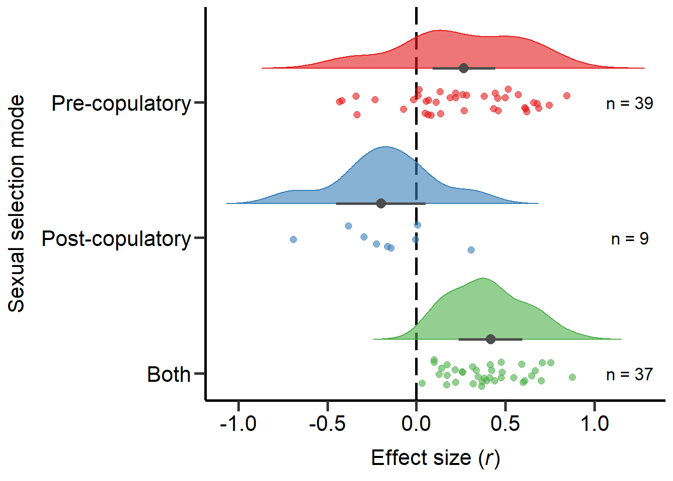

Figure 2: Raincloud plot of correlation coefficients between SSD and the modes of sexual selection proxies (i.e. pre-copulatory, post-copulatory or both) including sample sizes and estimates with 95%CI from phylogenetic model.

Sexual selection category

Next we explored the effect of the sexual selection category (i.e. density, mating system, operational sex ratio (OSR), post-mating competition, pre-mating competition, trait-based, other):

MetaData$SexSel_Category=as.factor(MetaData$SexSel_Category)
MetaData$SexSel_Category=relevel(MetaData$SexSel_Category,c("Postmating competition"))
Model_REML_by_SexSelCat = rma.mv(r ~ factor(SexSel_Category), V=Var_r, data = MetaData, random = c(~ 1 | Study_ID,~ 1 | Index, ~ 1 | Class), R = list(Class = forcedC_Moderators), method = "REML")
summary(Model_REML_by_SexSelCat)


Multivariate Meta-Analysis Model (k = 85; method: REML)

  logLik  Deviance       AIC       BIC      AICc   
  1.0179   -2.0359   17.9641   41.5312   21.2477   

Variance Components:

            estim    sqrt  nlvls  fixed    factor    R 
sigma^2.1  0.0198  0.1408     51     no  Study_ID   no 
sigma^2.2  0.0236  0.1537     85     no     Index   no 
sigma^2.3  0.0153  0.1237      9     no     Class  yes 

Test for Residual Heterogeneity:
QE(df = 78) = 765.4567, p-val < .0001

Test of Moderators (coefficients 2:7):
QM(df = 6) = 73.6003, p-val < .0001

Model Results:

                                              estimate      se     zval    pval 
intrcpt                                        -0.2144  0.1185  -1.8089  0.0705 
factor(SexSel_Category)Density                  0.4286  0.1396   3.0693  0.0021 
factor(SexSel_Category)Mating system            0.5918  0.1040   5.6922  <.0001 
factor(SexSel_Category)OSR                      0.8227  0.1472   5.5885  <.0001 
factor(SexSel_Category)Other                    0.5517  0.1194   4.6193  <.0001 
factor(SexSel_Category)Premating competition    0.5686  0.1042   5.4557  <.0001 
factor(SexSel_Category)Trait-based              0.1550  0.1167   1.3280  0.1842 
                                                ci.lb   ci.ub      
intrcpt                                       -0.4466  0.0179    . 
factor(SexSel_Category)Density                 0.1549  0.7023   ** 
factor(SexSel_Category)Mating system           0.3881  0.7956  *** 
factor(SexSel_Category)OSR                     0.5342  1.1113  *** 
factor(SexSel_Category)Other                   0.3176  0.7858  *** 
factor(SexSel_Category)Premating competition   0.3643  0.7728  *** 
factor(SexSel_Category)Trait-based            -0.0737  0.3837      

---
Signif. codes:  0 '***' 0.001 '**' 0.01 '*' 0.05 '.' 0.1 ' ' 1

We then re-leveled the model for post-hoc comparisons:

MetaData$SexSel_Category=relevel(MetaData$SexSel_Category,c("Trait-based"))
Model_REML_by_SexSelCat2 = rma.mv(r ~ factor(SexSel_Category), V=Var_r, data = MetaData, random = c(~ 1 | Study_ID,~ 1 | Index, ~ 1 | Class), R = list(Class = forcedC_Moderators), method = "REML")
summary(Model_REML_by_SexSelCat2)

MetaData$SexSel_Category=relevel(MetaData$SexSel_Category,c("Density"))
Model_REML_by_SexSelCat3 = rma.mv(r ~ factor(SexSel_Category), V=Var_r, data = MetaData, random = c(~ 1 | Study_ID,~ 1 | Index, ~ 1 | Class), R = list(Class = forcedC_Moderators), method = "REML")
summary(Model_REML_by_SexSelCat3)

MetaData$SexSel_Category=relevel(MetaData$SexSel_Category,c("Premating competition"))
Model_REML_by_SexSelCat4 = rma.mv(r ~ factor(SexSel_Category), V=Var_r, data = MetaData, random = c(~ 1 | Study_ID,~ 1 | Index, ~ 1 | Class), R = list(Class = forcedC_Moderators), method = "REML")
summary(Model_REML_by_SexSelCat4)

MetaData$SexSel_Category=relevel(MetaData$SexSel_Category,c("Mating system"))
Model_REML_by_SexSelCat5 = rma.mv(r ~ factor(SexSel_Category), V=Var_r, data = MetaData, random = c(~ 1 | Study_ID,~ 1 | Index, ~ 1 | Class), R = list(Class = forcedC_Moderators), method = "REML")
summary(Model_REML_by_SexSelCat5)

MetaData$SexSel_Category=relevel(MetaData$SexSel_Category,c("OSR"))
Model_REML_by_SexSelCat6 = rma.mv(r ~ factor(SexSel_Category), V=Var_r, data = MetaData, random = c(~ 1 | Study_ID,~ 1 | Index, ~ 1 | Class), R = list(Class = forcedC_Moderators), method = "REML")
summary(Model_REML_by_SexSelCat6)

MetaData$SexSel_Category=relevel(MetaData$SexSel_Category,c("Other"))
Model_REML_by_SexSelCat7 = rma.mv(r ~ factor(SexSel_Category), V=Var_r, data = MetaData, random = c(~ 1 | Study_ID,~ 1 | Index, ~ 1 | Class), R = list(Class = forcedC_Moderators), method = "REML")
summary(Model_REML_by_SexSelCat7)

Finally, we computed FDR corrected p-values:

tab2=as.data.frame(round(p.adjust(c(0.0705, 0.5745, 0.1057, 0.0002, .0001, .0001, 0.0011), method = 'fdr'),digit=3),row.names=cbind("Postmating competition","Trait-based","Density",'Premating competition',"Mating system","OSR","Other"))
colnames(tab2)<-cbind('P-value')
tab2

                       P-value
Postmating competition   0.099
Trait-based              0.575
Density                  0.123
Premating competition    0.000
Mating system            0.000
OSR                      0.000
Other                    0.002

Plot sexual selection category (Figure S1)

Here we plot the sexual selection category moderator:

MetaData$SexSel_Category=factor(MetaData$SexSel_Category, levels = rev(c( "Postmating competition","Trait-based" ,"Density","Premating competition" ,"Mating system" , "OSR", "Other")))

ggplot(MetaData, aes(x=SexSel_Category, y=r, fill = SexSel_Category, colour = SexSel_Category)) +
  geom_hline(yintercept=0, linetype="longdash", color = "black", linewidth=1)+
  geom_flat_violin(position = position_nudge(x = 0.25, y = 0),adjust =1, trim = F,alpha=0.6)+
  geom_point(position = position_jitter(width = .1), size = 2.5,alpha=0.6,stroke=0,shape=19)+
  geom_point(inherit.aes = F,mapping = aes(y=Model_REML_by_SexSelCat$b[1,1], x=7.25), size = 3.5,alpha=1,stroke=0,shape=19,color='grey30')+
  geom_point(inherit.aes = F,mapping = aes(y=Model_REML_by_SexSelCat2$b[1,1], x=6.25), size = 3.5,alpha=1,stroke=0,shape=19,color='grey30')+
  geom_point(inherit.aes = F,mapping = aes(y=Model_REML_by_SexSelCat3$b[1,1], x=5.25), size = 3.5,alpha=1,stroke=0,shape=19,color='grey30')+
  geom_point(inherit.aes = F,mapping = aes(y=Model_REML_by_SexSelCat4$b[1,1], x=4.25), size = 3.5,alpha=1,stroke=0,shape=19,color='grey30')+
  geom_point(inherit.aes = F,mapping = aes(y=Model_REML_by_SexSelCat5$b[1,1], x=3.25), size = 3.5,alpha=1,stroke=0,shape=19,color='grey30')+
  geom_point(inherit.aes = F,mapping = aes(y=Model_REML_by_SexSelCat6$b[1,1], x=2.25), size = 3.5,alpha=1,stroke=0,shape=19,color='grey30')+
  geom_point(inherit.aes = F,mapping = aes(y=Model_REML_by_SexSelCat7$b[1,1], x=1.25), size = 3.5,alpha=1,stroke=0,shape=19,color='grey30')+
  geom_segment(inherit.aes = F,mapping = aes(y=Model_REML_by_SexSelCat$ci.lb[1], x=7.25, xend= 7.25, yend= Model_REML_by_SexSelCat$ci.ub[1]), alpha=1,linewidth=1,color='grey30')+
  geom_segment(inherit.aes = F,mapping = aes(y=Model_REML_by_SexSelCat2$ci.lb[1], x=6.25, xend= 6.25, yend= Model_REML_by_SexSelCat2$ci.ub[1]), alpha=1,linewidth=1,color='grey30')+
  geom_segment(inherit.aes = F,mapping = aes(y=Model_REML_by_SexSelCat3$ci.lb[1], x=5.25, xend= 5.25, yend= Model_REML_by_SexSelCat3$ci.ub[1]), alpha=1,linewidth=1,color='grey30')+
  geom_segment(inherit.aes = F,mapping = aes(y=Model_REML_by_SexSelCat4$ci.lb[1], x=4.25, xend= 4.25, yend= Model_REML_by_SexSelCat4$ci.ub[1]), alpha=1,linewidth=1,color='grey30')+
  geom_segment(inherit.aes = F,mapping = aes(y=Model_REML_by_SexSelCat5$ci.lb[1], x=3.25, xend= 3.25, yend= Model_REML_by_SexSelCat5$ci.ub[1]), alpha=1,linewidth=1,color='grey30')+
  geom_segment(inherit.aes = F,mapping = aes(y=Model_REML_by_SexSelCat6$ci.lb[1], x=2.25, xend= 2.25, yend= Model_REML_by_SexSelCat6$ci.ub[1]), alpha=1,linewidth=1,color='grey30')+
  geom_segment(inherit.aes = F,mapping = aes(y=Model_REML_by_SexSelCat7$ci.lb[1], x=1.25, xend= 1.25, yend= Model_REML_by_SexSelCat7$ci.ub[1]), alpha=1,linewidth=1,color='grey30')+
  ylab(expression(paste("Effect size (", italic("r"),')')))+xlab('Sexual selection category')+coord_flip()+guides(fill = FALSE, colour = FALSE) +
  scale_color_manual(values =colpal2)+
  scale_fill_manual(values =colpal2)+
  scale_x_discrete(labels=rev(c( "Post-mating\ncompetition","Trait-based" ,"Density","Pre-mating\ncompetition" ,"Mating\nsystem" , "OSR", "Other")),expand=c(.1,0))+
  annotate("text", x=7, y=1.2, label= "n = 9",size=4.5) +
  annotate("text", x=6, y=1.2, label= "n = 12",size=4.5) +
  annotate("text", x=5, y=1.2, label= "n = 5",size=4.5) +
  annotate("text", x=4, y=1.2, label= "n = 18",size=4.5) +
  annotate("text", x=3, y=1.2, label= "n = 23",size=4.5) +
  annotate("text", x=2, y=1.2, label= "n = 6",size=4.5) +
  annotate("text", x=1, y=1.2, label= "n = 12",size=4.5) + theme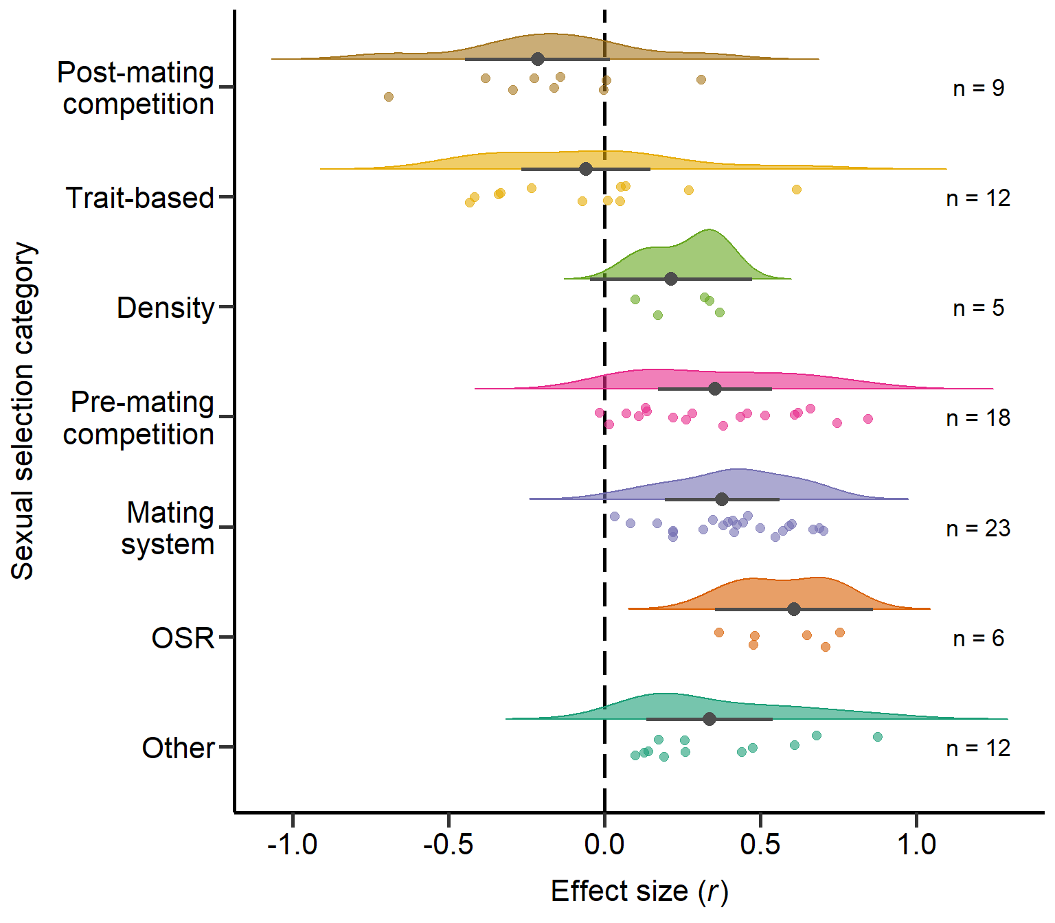

Figure S1: Raincloud plot of correlation coefficients between SSD and different sexual selection categories including sample sizes and estimates with 95%CI from phylogenetic model.

Type of SSD measure

Next we explored the effect of the type of SSD measure (i.e. body mass or size):

MetaData$SSD_Proxy=as.factor(MetaData$SSD_Proxy)
MetaData$SSD_Proxy=relevel(MetaData$SSD_Proxy,c("Body mass"))
Model_REML_by_SSDMeasure = rma.mv(r ~ SSD_Proxy, V=Var_r, data = MetaData, random = c(~ 1 | Study_ID,~ 1 | Index, ~ 1 | Class), R = list(Class = forcedC_Moderators), method = "REML")
summary(Model_REML_by_SSDMeasure)


Multivariate Meta-Analysis Model (k = 83; method: REML)

  logLik  Deviance       AIC       BIC      AICc   
-23.9277   47.8554   57.8554   69.8276   58.6554   

Variance Components:

            estim    sqrt  nlvls  fixed    factor    R 
sigma^2.1  0.0277  0.1664     50     no  Study_ID   no 
sigma^2.2  0.0633  0.2516     83     no     Index   no 
sigma^2.3  0.0097  0.0985      9     no     Class  yes 

Test for Residual Heterogeneity:
QE(df = 81) = 1404.5159, p-val < .0001

Test of Moderators (coefficient 2):
QM(df = 1) = 1.0294, p-val = 0.3103

Model Results:

                    estimate      se     zval    pval    ci.lb   ci.ub      
intrcpt               0.3582  0.1008   3.5543  0.0004   0.1607  0.5557  *** 
SSD_ProxyBody size   -0.0934  0.0920  -1.0146  0.3103  -0.2737  0.0870      

---
Signif. codes:  0 '***' 0.001 '**' 0.01 '*' 0.05 '.' 0.1 ' ' 1

We then re-leveled the model for post-hoc comparisons:

MetaData$SSD_Proxy=relevel(MetaData$SSD_Proxy,c("Body size"))
Model_REML_by_SSDMeasure2 = rma.mv(r ~ SSD_Proxy, V=Var_r, data = MetaData, random = c(~ 1 | Study_ID,~ 1 | Index, ~ 1 | Class), R = list(Class = forcedC_Moderators), method = "REML")
summary(Model_REML_by_SSDMeasure2)

Finally, we computed FDR corrected p-values:

tab3=as.data.frame(round(p.adjust(c(0.0004, 0.0008), method = 'fdr'),digit=3),row.names=cbind("Body mass","Body size"))
colnames(tab3)<-cbind('P-value')
tab3

          P-value
Body mass   0.001
Body size   0.001

Plot Type of SSD measure (Figure S2A)

Here we plot the type of SSD measure moderator:

MetaData_NAProxy=MetaData[!is.na(MetaData$SSD_Proxy),]
MetaData_NAProxy$SSD_Proxy=as.factor(MetaData_NAProxy$SSD_Proxy)
MetaData_NAProxy$SSD_Proxy=relevel(MetaData_NAProxy$SSD_Proxy,c("Body size"))

ggplot(MetaData_NAProxy, aes(x=SSD_Proxy, y=r, fill = SSD_Proxy, colour = SSD_Proxy)) +
  geom_hline(yintercept=0, linetype="longdash", color = "black", linewidth=1)+
  geom_flat_violin(position = position_nudge(x = 0.25, y = 0),adjust =1, trim = F,alpha=0.6)+
  geom_point(position = position_jitter(width = .1), size = 2.5,alpha=0.6,stroke=0,shape=19)+
  geom_point(inherit.aes = F,mapping = aes(y=Model_REML_by_SSDMeasure$b[1,1], x=2.25), size = 3.5,alpha=1,stroke=0,shape=19,color='grey30')+
  geom_point(inherit.aes = F,mapping = aes(y=Model_REML_by_SSDMeasure2$b[1,1], x=1.25), size = 3.5,alpha=1,stroke=0,shape=19,color='grey30')+
  geom_segment(inherit.aes = F,mapping = aes(y=Model_REML_by_SSDMeasure$ci.lb[1], x=2.25, xend= 2.25, yend= Model_REML_by_SSDMeasure$ci.ub[1]), alpha=1,linewidth=1,color='grey30')+
  geom_segment(inherit.aes = F,mapping = aes(y=Model_REML_by_SSDMeasure2$ci.lb[1], x=1.25, xend= 1.25, yend= Model_REML_by_SSDMeasure2$ci.ub[1]), alpha=1,linewidth=1,color='grey30')+
  ylab(expression(paste("Effect size (", italic("r"),')')))+xlab('Type of SSD measure')+coord_flip()+guides(fill = FALSE, colour = FALSE) +
  scale_color_manual(values =colpal4)+
  scale_fill_manual(values =colpal4)+
  scale_x_discrete(labels=rev(c("Body mass","Body size")),expand=c(.15,0))+
  annotate("text", x=2, y=1.2, label= "n = 37",size=4.5) +
  annotate("text", x=1, y=1.2, label= "n = 46",size=4.5)  + theme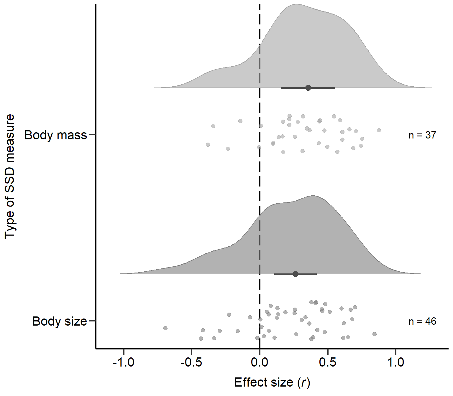

Figure S2A: Raincloud plot of correlation coefficients for different types of SSD measures (i.e. body mass or size) including sample sizes and estimates with 95% CI from phylogenetic model.

SSD measure controlled for body size?

Next we explored the effect if the primary study controlled the SSD for body size (i.e. uncontrolled or controlled):

MetaData$BodySizeControlled=as.factor(MetaData$BodySizeControlled)
MetaData$BodySizeControlled=relevel(MetaData$BodySizeControlled,c("No"))
Model_REML_by_BodySizeCont = rma.mv(r ~ BodySizeControlled, V=Var_r, data = MetaData, random = c(~ 1 | Study_ID,~ 1 | Index, ~ 1 | Class), R = list(Class = forcedC_Moderators), method = "REML")
summary(Model_REML_by_BodySizeCont)


Multivariate Meta-Analysis Model (k = 85; method: REML)

  logLik  Deviance       AIC       BIC      AICc   
-23.9319   47.8637   57.8637   69.9579   58.6430   

Variance Components:

            estim    sqrt  nlvls  fixed    factor    R 
sigma^2.1  0.0263  0.1622     51     no  Study_ID   no 
sigma^2.2  0.0619  0.2488     85     no     Index   no 
sigma^2.3  0.0147  0.1214      9     no     Class  yes 

Test for Residual Heterogeneity:
QE(df = 83) = 1445.3959, p-val < .0001

Test of Moderators (coefficient 2):
QM(df = 1) = 0.2803, p-val = 0.5965

Model Results:

                       estimate      se     zval    pval    ci.lb   ci.ub      
intrcpt                  0.3023  0.0885   3.4172  0.0006   0.1289  0.4757  *** 
BodySizeControlledYes   -0.0546  0.1031  -0.5294  0.5965  -0.2566  0.1474      

---
Signif. codes:  0 '***' 0.001 '**' 0.01 '*' 0.05 '.' 0.1 ' ' 1

We then re-leveled the model for post-hoc comparisons:

MetaData$BodySizeControlled=relevel(MetaData$BodySizeControlled,c("Yes"))
Model_REML_by_BodySizeCont2 = rma.mv(r ~ BodySizeControlled, V=Var_r, data = MetaData, random = c(~ 1 | Study_ID,~ 1 | Index, ~ 1 | Class), R = list(Class = forcedC_Moderators), method = "REML")
summary(Model_REML_by_BodySizeCont2)

Finally, we computed FDR corrected p-values:

tab4=as.data.frame(round(p.adjust(c(0.0006, 0.0337), method = 'fdr'),digit=3),row.names=cbind("uncontrolled","controlled"))
colnames(tab4)<-cbind('P-value')
tab4

             P-value
uncontrolled   0.001
controlled     0.034

Plot: SSD measure controlled for body size? (Figure S2B)

Here we plot effect sizes if type of SSD measure controlled for body size:

MetaData$BodySizeControlled=as.factor(MetaData$BodySizeControlled)
MetaData$BodySizeControlled=relevel(MetaData$BodySizeControlled,c("Yes"))

ggplot(MetaData, aes(x=BodySizeControlled, y=r, fill = BodySizeControlled, colour = BodySizeControlled)) +
  geom_hline(yintercept=0, linetype="longdash", color = "black", linewidth=1)+
  geom_flat_violin(position = position_nudge(x = 0.25, y = 0),adjust =1, trim = F,alpha=0.6)+
  geom_point(position = position_jitter(width = .1), size = 2.5,alpha=0.6,stroke=0,shape=19)+
  geom_point(inherit.aes = F,mapping = aes(y=Model_REML_by_BodySizeCont$b[1,1], x=2.25), size = 3.5,alpha=1,stroke=0,shape=19,color='grey30')+
  geom_point(inherit.aes = F,mapping = aes(y=Model_REML_by_BodySizeCont2$b[1,1], x=1.25), size = 3.5,alpha=1,stroke=0,shape=19,color='grey30')+
  geom_segment(inherit.aes = F,mapping = aes(y=Model_REML_by_BodySizeCont$ci.lb[1], x=2.25, xend= 2.25, yend= Model_REML_by_BodySizeCont$ci.ub[1]), alpha=1,linewidth=1,color='grey30')+
  geom_segment(inherit.aes = F,mapping = aes(y=Model_REML_by_BodySizeCont2$ci.lb[1], x=1.25, xend= 1.25, yend= Model_REML_by_BodySizeCont2$ci.ub[1]), alpha=1,linewidth=1,color='grey30')+
  ylab(expression(paste("Effect size (", italic("r"),')')))+xlab('SSD controlled for body size?')+coord_flip()+guides(fill = FALSE, colour = FALSE) +
  scale_color_manual(values =colpal4)+
  scale_fill_manual(values =colpal4)+
  scale_x_discrete(labels=(c("Controlled","Uncontrolled")),expand=c(.15,0))+
  annotate("text", x=2, y=1.2, label= "n = 69",size=4.5) +
  annotate("text", x=1, y=1.2, label= "n = 16",size=4.5)  + theme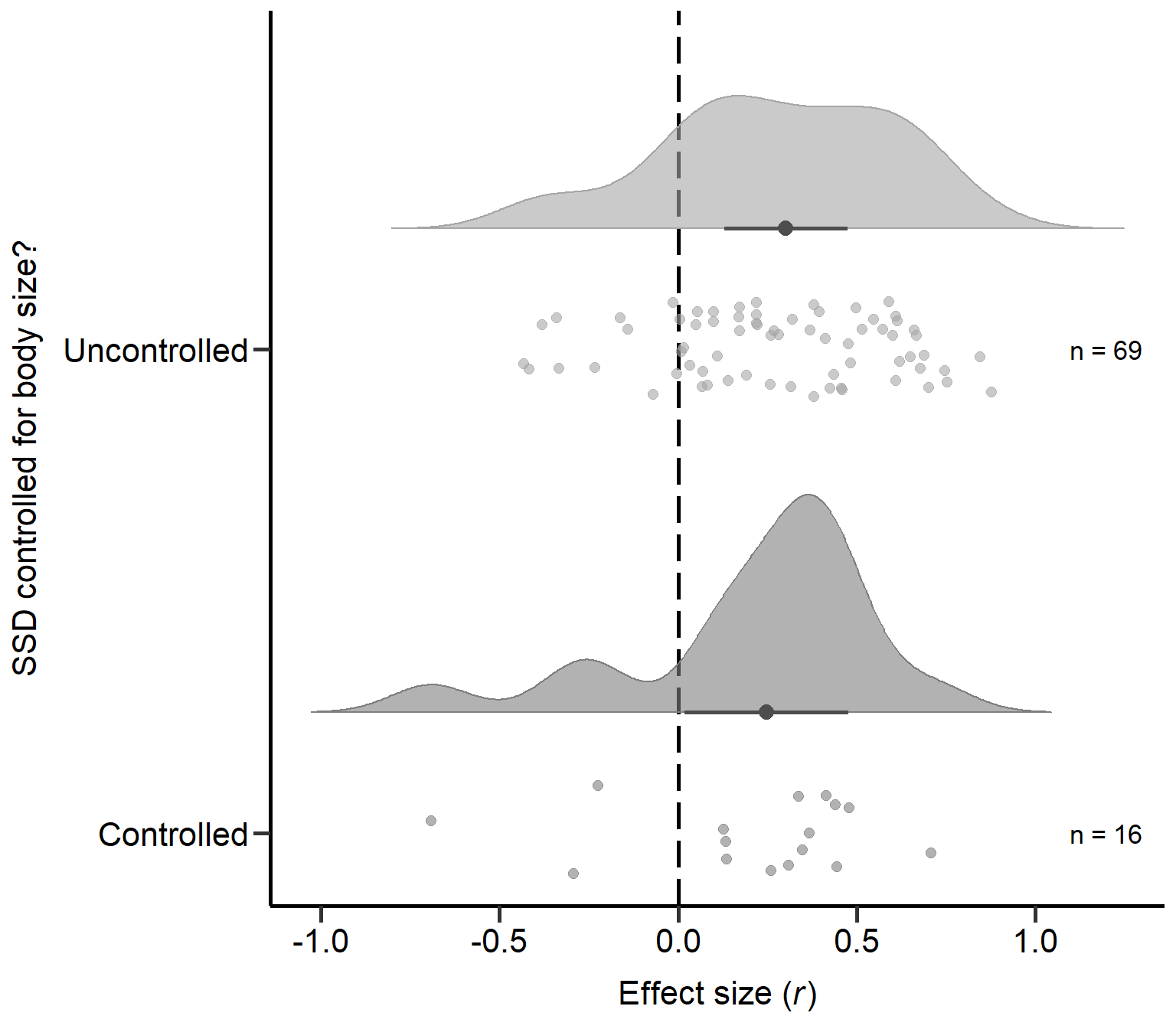

Figure S2B: Raincloud plot of correlation coefficients for primary studies controlling SSD for body size or mass (uncontrolled or controlled) including sample sizes and estimates with 95% CI from phylogenetic model.

Phylogentic vs non-phylogenetic studies

Next we explored the effect of studies controlling for phylogeny vs non-phylogenetic studies:

MetaData$PhyloControlled=as.factor(MetaData$PhyloControlled)
MetaData$PhyloControlled=relevel(MetaData$PhyloControlled,c("No"))
Model_cREML_by_Phylo = rma.mv(r ~ PhyloControlled, V=Var_r, data = MetaData, random = c(~ 1 | Study_ID,~ 1 | Index, ~ 1 | Class), R = list(Class = forcedC_Moderators), method = "REML")
summary(Model_cREML_by_Phylo)


Multivariate Meta-Analysis Model (k = 85; method: REML)

  logLik  Deviance       AIC       BIC      AICc   
-19.4587   38.9175   48.9175   61.0117   49.6967   

Variance Components:

            estim    sqrt  nlvls  fixed    factor    R 
sigma^2.1  0.0000  0.0000     51     no  Study_ID   no 
sigma^2.2  0.0724  0.2690     85     no     Index   no 
sigma^2.3  0.0203  0.1425      9     no     Class  yes 

Test for Residual Heterogeneity:
QE(df = 83) = 1214.8661, p-val < .0001

Test of Moderators (coefficient 2):
QM(df = 1) = 11.9815, p-val = 0.0005

Model Results:

                    estimate      se     zval    pval    ci.lb    ci.ub      
intrcpt               0.6301  0.1363   4.6222  <.0001   0.3629   0.8972  *** 
PhyloControlledYes   -0.3967  0.1146  -3.4614  0.0005  -0.6214  -0.1721  *** 

---
Signif. codes:  0 '***' 0.001 '**' 0.01 '*' 0.05 '.' 0.1 ' ' 1

We then re-leveled the model for post-hoc comparisons:

MetaData$PhyloControlled=relevel(MetaData$PhyloControlled,c("Yes"))
Model_cREML_by_Phylo2 = rma.mv(r ~ PhyloControlled, V=Var_r, data = MetaData, random = c(~ 1 | Study_ID,~ 1 | Index, ~ 1 | Class), R = list(Class = forcedC_Moderators), method = "REML")
summary(Model_cREML_by_Phylo2)

Finally, we computed FDR corrected p-values:

tab5=as.data.frame(round(p.adjust(c(0.0001, 0.0096), method = 'fdr'),digit=3),row.names=cbind("Non-phylogenetic","With phylogeny"))
colnames(tab5)<-cbind('P-value')
tab5

                 P-value
Non-phylogenetic    0.00
With phylogeny      0.01

Plot Phylogentic vs non-phylogenetic studies (Figure S2C)

Here we plot the type of SSD measure moderator:

MetaData$PhyloControlled=as.factor(MetaData$PhyloControlled)
MetaData$PhyloControlled=relevel(MetaData$PhyloControlled,c("No"))

ggplot(MetaData, aes(x=PhyloControlled, y=r, fill = PhyloControlled, colour = PhyloControlled)) +
  geom_hline(yintercept=0, linetype="longdash", color = "black", linewidth=1)+
  geom_flat_violin(position = position_nudge(x = 0.25, y = 0),adjust =1, trim = F,alpha=0.6)+
  geom_point(position = position_jitter(width = .1), size = 2.5,alpha=0.6,stroke=0,shape=19)+
  geom_point(inherit.aes = F,mapping = aes(y=Model_cREML_by_Phylo2$b[1,1], x=2.25), size = 3.5,alpha=1,stroke=0,shape=19,color='grey30')+
  geom_point(inherit.aes = F,mapping = aes(y=Model_cREML_by_Phylo$b[1,1], x=1.25), size = 3.5,alpha=1,stroke=0,shape=19,color='grey30')+
  geom_segment(inherit.aes = F,mapping = aes(y=Model_cREML_by_Phylo2$ci.lb[1], x=2.25, xend= 2.25, yend= Model_cREML_by_Phylo2$ci.ub[1]), alpha=1,linewidth=1,color='grey30')+
  geom_segment(inherit.aes = F,mapping = aes(y=Model_cREML_by_Phylo$ci.lb[1], x=1.25, xend= 1.25, yend= Model_cREML_by_Phylo$ci.ub[1]), alpha=1,linewidth=1,color='grey30')+
  ylab(expression(paste("Effect size (", italic("r"),')')))+xlab('Type of analysis')+coord_flip()+guides(fill = FALSE, colour = FALSE) +
  scale_color_manual(values =colpal4)+
  scale_fill_manual(values =colpal4)+
  scale_x_discrete(labels=(c("Phylogenetically \n uncorrected ","Phylogenetically \n corrected ")),expand=c(.15,0))+
  annotate("text", x=1, y=1.2, label= "n = 8",size=4.5) +
  annotate("text", x=2, y=1.2, label= "n = 77",size=4.5)  + theme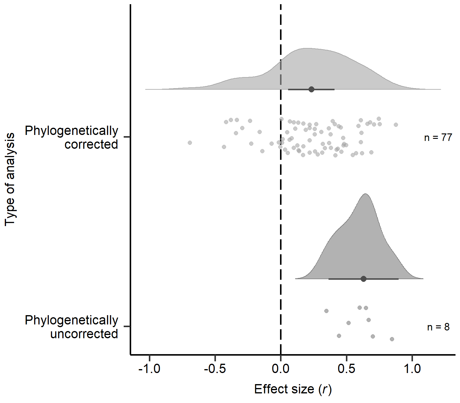

Figure S2C: Raincloud plot of correlation coefficients for non-phylogenetic and phylogenetic analyses in primary studies including sample sizes and estimates with 95% CI from phylogenetic model (Table 4).

Test for publication bias

To test for publication bias, we transformed r into z scores and ran multilevel mixed-effects models (restricted maximum likelihood) with z as the predictor and its standard error as the response with study ID and an observation level random effect. Models were weight by the mean standard error of z across all studies. While the variance in r depends on the effect size and the sample size, the variance in z is only dependent on the sample size. Hence, if z values correlate with the variance in z, this indicates that small studies were only published, if the effect was large, suggesting publication bias.

Model_REML_PublBias         = rma.mv(z ~ SE_z, V=rep((mean(SE_z)*mean(SE_z))*N,length(SE_z)), data = MetaData, random = c(~ 1 | Study_ID,~ 1 | Index, ~ 1 | Class), R = list(Class = forcedC_Moderators), method = "REML",control=list(rel.tol=1e-8))
summary(Model_REML_PublBias)


Multivariate Meta-Analysis Model (k = 85; method: REML)

   logLik   Deviance        AIC        BIC       AICc   
-101.0851   202.1703   212.1703   224.2645   212.9495   

Variance Components:

            estim    sqrt  nlvls  fixed    factor    R 
sigma^2.1  0.0000  0.0000     51     no  Study_ID   no 
sigma^2.2  0.0000  0.0000     85     no     Index   no 
sigma^2.3  0.0000  0.0003      9     no     Class  yes 

Test for Residual Heterogeneity:
QE(df = 83) = 14.4691, p-val = 1.0000

Test of Moderators (coefficient 2):
QM(df = 1) = 2.8672, p-val = 0.0904

Model Results:

         estimate      se    zval    pval    ci.lb   ci.ub    
intrcpt    0.0674  0.2533  0.2663  0.7900  -0.4290  0.5639    
SE_z       1.5228  0.8993  1.6933  0.0904  -0.2398  3.2854  . 

---
Signif. codes:  0 '***' 0.001 '**' 0.01 '*' 0.05 '.' 0.1 ' ' 1

Figure S2D

# Extract model predictions
model_p2 <- predict(Model_REML_PublBias)

ggplot(MetaData, aes(x=SE_z, y=z)) +
  theme(panel.grid.major = element_blank(), panel.grid.minor = element_blank(),panel.background = element_blank(), axis.line = element_line(colour = "black"))+
  theme(axis.text=element_text(size=13),
        axis.title=element_text(size=14))+ theme(legend.position="none")+ylab(expression(paste("Effect size (", italic("z"),')')))+
  geom_point(shape=16, size = 3,alpha=0.5)+xlab('Standard error')+
  geom_hline(yintercept=0, linetype="dashed", color = "black", linewidth=1)+
  geom_line( aes(y = model_p2$pred), size = 1)+ 
  geom_ribbon( aes(ymin = model_p2$ci.lb, ymax = model_p2$ci.ub, color = 'black',linetype=NA), alpha = .15,show.legend = F, outline.type = "both") +
  theme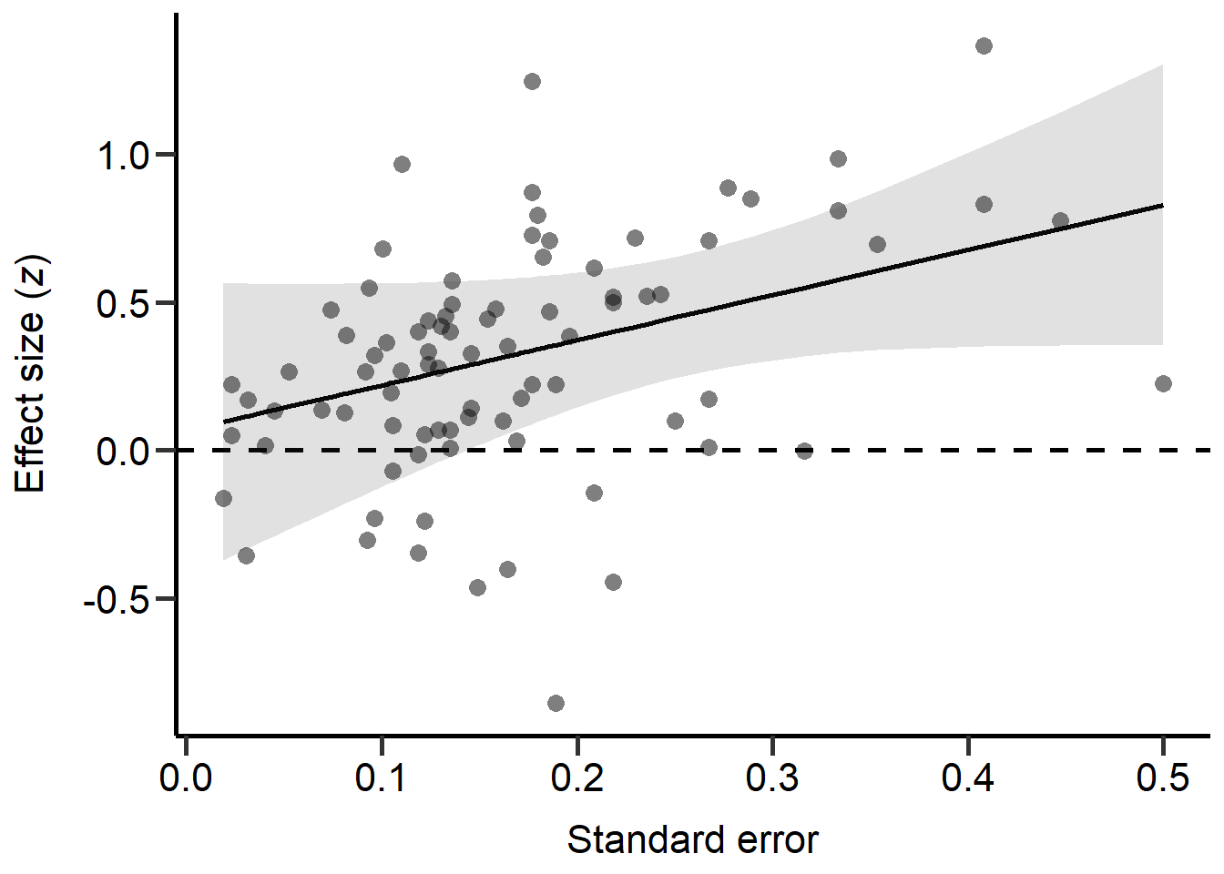

Figure S2D: Scatter plot of the standard error in z scores of each study against the z score of each primary study (transformed correlation coefficients). Dashed line marks a correlation coefficient of zero, black line represents predictions from REML model (controlling for phylogeny) and grey area represents 95% CI on model predictions.

Publication year

Next we explored the effect of the publication year of each study:

Model_REML_by_Year = rma.mv(r ~ Year, V=Var_r, data = MetaData, random = c(~ 1 | Study_ID,~ 1 | Index, ~ 1 | Class), R = list(Class = forcedC_Moderators), method = "REML")
summary(Model_REML_by_Year)


Multivariate Meta-Analysis Model (k = 85; method: REML)

  logLik  Deviance       AIC       BIC      AICc   
-21.5905   43.1810   53.1810   65.2752   53.9602   

Variance Components:

            estim    sqrt  nlvls  fixed    factor    R 
sigma^2.1  0.0160  0.1266     51     no  Study_ID   no 
sigma^2.2  0.0624  0.2498     85     no     Index   no 
sigma^2.3  0.0206  0.1435      9     no     Class  yes 

Test for Residual Heterogeneity:
QE(df = 83) = 1136.4440, p-val < .0001

Test of Moderators (coefficient 2):
QM(df = 1) = 5.5451, p-val = 0.0185

Model Results:

         estimate      se     zval    pval    ci.lb    ci.ub    
intrcpt   17.0962  7.1392   2.3947  0.0166   3.1037  31.0888  * 
Year      -0.0084  0.0036  -2.3548  0.0185  -0.0153  -0.0014  * 

---
Signif. codes:  0 '***' 0.001 '**' 0.01 '*' 0.05 '.' 0.1 ' ' 1

Plot publication year (Figure S2E)

Here we plot the publication year:

# Extract model predictions
Model_REML_by_Year = rma.mv(r ~ Year, V=Var_r, data = MetaData, random = c(~ 1 | Study_ID,~ 1 | Index, ~ 1 | Class), R = list(Class = forcedC_Moderators), method = "REML")
model_p4 <- predict(Model_REML_by_Year)

ggplot(MetaData, aes(x=as.numeric(Year), y=r)) +
  theme(panel.grid.major = element_blank(), panel.grid.minor = element_blank(),panel.background = element_blank(), axis.line = element_line(colour = "black"))+
  theme(axis.text=element_text(size=13),
        axis.title=element_text(size=14))+ theme(legend.position="none")+
  geom_point(shape=16, size = 3,alpha=0.5)+xlab('Publication year')+ylab(expression(paste("Effect size (", italic("r"),')')))+
  geom_hline(yintercept=0, linetype="dashed", color = "black", linewidth=1)+
  geom_line( aes(y = model_p4$pred), size = 1)+ 
  geom_ribbon( aes(ymin = model_p4$ci.lb, ymax = model_p4$ci.ub, color = 'black',linetype=NA), alpha = .15,show.legend = F, outline.type = "both") +
  theme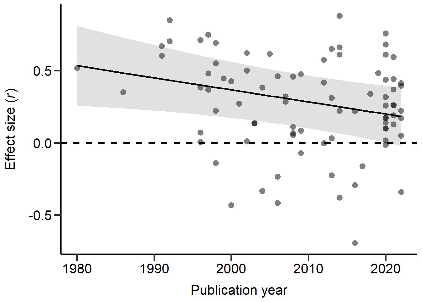

Figure S2E: Scatter plot of correlation coefficients against the publication year of each study. Dashed line marks a correlation coefficient of zero, black line represents predictions from REML model (controlling for phylogeny) and grey area represents 95% CI on model predictions.

Moderator tests for non-phylogenetic models

Here we ran all models without the phylogeny.

Sexual selection mode

The first model explores the effect of the sexual selection mode (i.e. pre-copulatory, post-copulatory or both):

MetaData$SexSel_Mode=relevel(MetaData$SexSel_Mode,c("pre-copulatory"))
Model_REML_by_cSexSelMode = rma.mv(r ~ factor(SexSel_Mode), V=Var_r, data = MetaData, random = c(~ 1 | Study_ID,~ 1 | Index), method = "REML")
summary(Model_REML_by_cSexSelMode)


Multivariate Meta-Analysis Model (k = 85; method: REML)

  logLik  Deviance       AIC       BIC      AICc   
-13.2317   26.4634   36.4634   48.4970   37.2529   

Variance Components:

            estim    sqrt  nlvls  fixed    factor 
sigma^2.1  0.0225  0.1501     51     no  Study_ID 
sigma^2.2  0.0471  0.2171     85     no     Index 

Test for Residual Heterogeneity:
QE(df = 82) = 1230.9203, p-val < .0001

Test of Moderators (coefficients 2:3):
QM(df = 2) = 27.7973, p-val < .0001

Model Results:

                                    estimate      se     zval    pval    ci.lb 
intrcpt                               0.2592  0.0492   5.2684  <.0001   0.1628 
factor(SexSel_Mode)both               0.1603  0.0683   2.3468  0.0189   0.0264 
factor(SexSel_Mode)post-copulatory   -0.4444  0.1135  -3.9136  <.0001  -0.6669 
                                      ci.ub      
intrcpt                              0.3556  *** 
factor(SexSel_Mode)both              0.2942    * 
factor(SexSel_Mode)post-copulatory  -0.2218  *** 

---
Signif. codes:  0 '***' 0.001 '**' 0.01 '*' 0.05 '.' 0.1 ' ' 1

We then re-leveled the model for post-hoc comparisons:

MetaData$SexSel_Mode=relevel(MetaData$SexSel_Mode,c("post-copulatory"))
Model_REML_by_cSexSelMode2 = rma.mv(r ~ factor(SexSel_Mode), V=Var_r, data = MetaData, random = c(~ 1 | Study_ID,~ 1 | Index), method = "REML")
summary(Model_REML_by_cSexSelMode2)

MetaData$SexSel_Mode=relevel(MetaData$SexSel_Mode,c("both"))
Model_REML_by_cSexSelMode3 = rma.mv(r ~ factor(SexSel_Mode), V=Var_r, data = MetaData, random = c(~ 1 | Study_ID,~ 1 | Index),  method = "REML")
summary(Model_REML_by_cSexSelMode3)

Finally, we computed FDR corrected p-values:

tab1=as.data.frame(round(p.adjust(c(0.0001, 0.0756, .0001), method = 'fdr'),digit=3),row.names=cbind("Pre-copulatory","Post-copulatory","Both"))
colnames(tab1)<-cbind('P-value')
tab1

                P-value
Pre-copulatory    0.000
Post-copulatory   0.076
Both              0.000

Sexual selection category

Next we explored the effect of the sexual selection category (i.e. density, mating system, operational sex ratio (OSR), post-mating competition, pre-mating competition, trait-based, other):

MetaData$SexSel_Category=as.factor(MetaData$SexSel_Category)
MetaData$SexSel_Category=relevel(MetaData$SexSel_Category,c("Postmating competition"))
Model_REML_by_cSexSelCat = rma.mv(r ~ factor(SexSel_Category), V=Var_r, data = MetaData, random = c(~ 1 | Study_ID,~ 1 | Index), method = "REML")
summary(Model_REML_by_cSexSelCat)


Multivariate Meta-Analysis Model (k = 85; method: REML)

  logLik  Deviance       AIC       BIC      AICc   
  0.1558   -0.3116   17.6884   38.8988   20.3355   

Variance Components:

            estim    sqrt  nlvls  fixed    factor 
sigma^2.1  0.0250  0.1582     51     no  Study_ID 
sigma^2.2  0.0247  0.1571     85     no     Index 

Test for Residual Heterogeneity:
QE(df = 78) = 765.4567, p-val < .0001

Test of Moderators (coefficients 2:7):
QM(df = 6) = 73.2651, p-val < .0001

Model Results:

                                              estimate      se     zval    pval 
intrcpt                                        -0.1685  0.0925  -1.8218  0.0685 
factor(SexSel_Category)Other                    0.5532  0.1212   4.5647  <.0001 
factor(SexSel_Category)OSR                      0.8048  0.1462   5.5046  <.0001 
factor(SexSel_Category)Mating system            0.5855  0.1043   5.6126  <.0001 
factor(SexSel_Category)Premating competition    0.5553  0.1072   5.1809  <.0001 
factor(SexSel_Category)Density                  0.4346  0.1428   3.0429  0.0023 
factor(SexSel_Category)Trait-based              0.1317  0.1154   1.1418  0.2535 
                                                ci.lb   ci.ub      
intrcpt                                       -0.3498  0.0128    . 
factor(SexSel_Category)Other                   0.3156  0.7907  *** 
factor(SexSel_Category)OSR                     0.5183  1.0914  *** 
factor(SexSel_Category)Mating system           0.3810  0.7899  *** 
factor(SexSel_Category)Premating competition   0.3452  0.7653  *** 
factor(SexSel_Category)Density                 0.1547  0.7146   ** 
factor(SexSel_Category)Trait-based            -0.0944  0.3578      

---
Signif. codes:  0 '***' 0.001 '**' 0.01 '*' 0.05 '.' 0.1 ' ' 1

We then re-leveled the model for post-hoc comparisons:

MetaData$SexSel_Category=relevel(MetaData$SexSel_Category,c("Trait-based"))
Model_REML_by_cSexSelCat2 = rma.mv(r ~ factor(SexSel_Category), V=Var_r, data = MetaData, random = c(~ 1 | Study_ID,~ 1 | Index), method = "REML")
summary(Model_REML_by_cSexSelCat2)

MetaData$SexSel_Category=relevel(MetaData$SexSel_Category,c("Density"))
Model_REML_by_cSexSelCat3 = rma.mv(r ~ factor(SexSel_Category), V=Var_r, data = MetaData, random = c(~ 1 | Study_ID,~ 1 | Index), method = "REML")
summary(Model_REML_by_cSexSelCat3)

MetaData$SexSel_Category=relevel(MetaData$SexSel_Category,c("Premating competition"))
Model_REML_by_cSexSelCat4 = rma.mv(r ~ factor(SexSel_Category), V=Var_r, data = MetaData, random = c(~ 1 | Study_ID,~ 1 | Index), method = "REML")
summary(Model_REML_by_cSexSelCat4)

MetaData$SexSel_Category=relevel(MetaData$SexSel_Category,c("Mating system"))
Model_REML_by_cSexSelCat5 = rma.mv(r ~ factor(SexSel_Category), V=Var_r, data = MetaData, random = c(~ 1 | Study_ID,~ 1 | Index), method = "REML")
summary(Model_REML_by_cSexSelCat5)

MetaData$SexSel_Category=relevel(MetaData$SexSel_Category,c("OSR"))
Model_REML_by_cSexSelCat6 = rma.mv(r ~ factor(SexSel_Category), V=Var_r, data = MetaData, random = c(~ 1 | Study_ID,~ 1 | Index), method = "REML")
summary(Model_REML_by_cSexSelCat6)

MetaData$SexSel_Category=relevel(MetaData$SexSel_Category,c("Other"))
Model_REML_by_cSexSelCat7 = rma.mv(r ~ factor(SexSel_Category), V=Var_r, data = MetaData, random = c(~ 1 | Study_ID,~ 1 | Index), method = "REML")
summary(Model_REML_by_cSexSelCat7)

Finally, we computed FDR corrected p-values:

tab2=as.data.frame(round(p.adjust(c(0.0685, 0.5996, 0.0151, .0001, .0001, .0001, .0001), method = 'fdr'),digit=3),row.names=cbind("Postmating competition","Trait-based","Density",'Premating competition',"Mating system","OSR","Other"))
colnames(tab2)<-cbind('P-value')
tab2

                       P-value
Postmating competition   0.080
Trait-based              0.600
Density                  0.021
Premating competition    0.000
Mating system            0.000
OSR                      0.000
Other                    0.000

Phylogenetic classes

Next we explored the effect of the phylogenetic classes:

MetaData$Class=as.factor(MetaData$Class)
MetaData$Class=relevel(MetaData$Class,c("Nematoda"))
Model_cREML_by_Class = rma.mv(r ~ Class, V=Var_r, data = MetaData, random = c(~ 1 | Study_ID,~ 1 | Index), method = "REML")
summary(Model_cREML_by_Class)


Multivariate Meta-Analysis Model (k = 85; method: REML)

  logLik  Deviance       AIC       BIC      AICc   
-20.3784   40.7568   62.7568   88.3949   66.8818   

Variance Components:

            estim    sqrt  nlvls  fixed    factor 
sigma^2.1  0.0289  0.1701     51     no  Study_ID 
sigma^2.2  0.0615  0.2480     85     no     Index 

Test for Residual Heterogeneity:
QE(df = 76) = 1105.0314, p-val < .0001

Test of Moderators (coefficients 2:9):
QM(df = 8) = 11.1317, p-val = 0.1943

Model Results:

                     estimate      se     zval    pval    ci.lb   ci.ub    
intrcpt                0.4221  0.2716   1.5538  0.1202  -0.1103  0.9545    
ClassActinopterygii   -0.2496  0.3112  -0.8022  0.4225  -0.8594  0.3603    
ClassAmphibia         -0.2907  0.3233  -0.8992  0.3685  -0.9243  0.3429    
ClassAnimalia         -0.1962  0.3722  -0.5271  0.5981  -0.9257  0.5333    
ClassAves             -0.2221  0.2807  -0.7912  0.4288  -0.7724  0.3281    
ClassInsecta           0.0288  0.3069   0.0939  0.9252  -0.5727  0.6304    
ClassMammalia         -0.0056  0.2799  -0.0200  0.9840  -0.5542  0.5430    
ClassPisces           -0.1638  0.4082  -0.4012  0.6883  -0.9639  0.6363    
ClassReptilia         -0.3315  0.2959  -1.1203  0.2626  -0.9115  0.2485    

---
Signif. codes:  0 '***' 0.001 '**' 0.01 '*' 0.05 '.' 0.1 ' ' 1

We then re-leveled the model for post-hoc comparisons:

MetaData$Class=relevel(MetaData$Class,c("Insecta"))
Model_cREML_by_Class2 = rma.mv(r ~ Class, V=Var_r, data = MetaData, random = c(~ 1 | Study_ID,~ 1 | Index), method = "REML")
summary(Model_cREML_by_Class2)

MetaData$Class=relevel(MetaData$Class,c("Aves"))
Model_cREML_by_Class3 = rma.mv(r ~ Class, V=Var_r, data = MetaData, random = c(~ 1 | Study_ID,~ 1 | Index), method = "REML")
summary(Model_cREML_by_Class3)

MetaData$Class=relevel(MetaData$Class,c("Reptilia"))
Model_cREML_by_Class4 = rma.mv(r ~ Class, V=Var_r, data = MetaData, random = c(~ 1 | Study_ID,~ 1 | Index), method = "REML")
summary(Model_cREML_by_Class4)

MetaData$Class=relevel(MetaData$Class,c("Mammalia"))
Model_cREML_by_Class5 = rma.mv(r ~ Class, V=Var_r, data = MetaData, random = c(~ 1 | Study_ID,~ 1 | Index), method = "REML")
summary(Model_cREML_by_Class5)

MetaData$Class=relevel(MetaData$Class,c("Amphibia"))
Model_cREML_by_Class6 = rma.mv(r ~ Class, V=Var_r, data = MetaData, random = c(~ 1 | Study_ID,~ 1 | Index), method = "REML")
summary(Model_cREML_by_Class6)

MetaData$Class=relevel(MetaData$Class,c("Actinopterygii"))
Model_cREML_by_Class7 = rma.mv(r ~ Class, V=Var_r, data = MetaData, random = c(~ 1 | Study_ID,~ 1 | Index), method = "REML")
summary(Model_cREML_by_Class7)


MetaData$Class=relevel(MetaData$Class,c("Pisces"))
Model_cREML_by_Class8 = rma.mv(r ~ Class, V=Var_r, data = MetaData, random = c(~ 1 | Study_ID,~ 1 | Index), method = "REML")
summary(Model_cREML_by_Class8)

MetaData$Class=relevel(MetaData$Class,c("Animalia"))
Model_cREML_by_Class9 = rma.mv(r ~ Class, V=Var_r, data = MetaData, random = c(~ 1 | Study_ID,~ 1 | Index), method = "REML")
summary(Model_cREML_by_Class9)

Finally, we computed FDR corrected p-values:

tab2=as.data.frame(round(p.adjust(c(0.2557       ,0.4534     , 0.3747    ,0.0048    ,0.0016    ,.0001  ,0.1202    , 0.3966  ,0.4405       ), method = 'fdr'),digit=3),row.names=cbind( "Nematoda","Insecta","Aves","Reptilia","Mammalia","Amphibia","Actinopterygii","Pisces","Animalia"))
colnames(tab2)<-cbind('P-value')
tab2

               P-value
Nematoda         0.453
Insecta          0.453
Aves             0.453
Reptilia         0.014
Mammalia         0.007
Amphibia         0.001
Actinopterygii   0.270
Pisces           0.453
Animalia         0.453

Plot phylogenetic classes (Figure 3)

Here we plot the phylogenetic classes:

MetaData$Class=as.factor(MetaData$Class)
MetaData$Class=factor(MetaData$Class, levels = (c("Animalia","Pisces" ,"Actinopterygii","Amphibia","Mammalia","Reptilia","Aves","Insecta","Nematoda")))

ggplot(MetaData, aes(x=Class, y=r, fill = Class, colour = Class)) +
  geom_hline(yintercept=0, linetype="longdash", color = "black", linewidth=1)+
  geom_point(position = position_jitter(width = .1), size = 2.5,alpha=0.8,stroke=0,shape=19)+
  geom_point(inherit.aes = F,mapping = aes(y=Model_cREML_by_Class$b[1,1], x=9.35), size = 3.5,alpha=1,stroke=0,shape=19,color=colpal3[9])+
  geom_point(inherit.aes = F,mapping = aes(y=Model_cREML_by_Class2$b[1,1], x=8.35), size = 3.5,alpha=1,stroke=0,shape=19,color=colpal3[8])+
  geom_point(inherit.aes = F,mapping = aes(y=Model_cREML_by_Class3$b[1,1], x=7.35), size = 3.5,alpha=1,stroke=0,shape=19,color=colpal3[7])+
  geom_point(inherit.aes = F,mapping = aes(y=Model_cREML_by_Class4$b[1,1], x=6.35), size = 3.5,alpha=1,stroke=0,shape=19,color=colpal3[6])+
  geom_point(inherit.aes = F,mapping = aes(y=Model_cREML_by_Class5$b[1,1], x=5.35), size = 3.5,alpha=1,stroke=0,shape=19,color=colpal3[5])+
  geom_point(inherit.aes = F,mapping = aes(y=Model_cREML_by_Class6$b[1,1], x=4.35), size = 3.5,alpha=1,stroke=0,shape=19,color=colpal3[4])+
  geom_point(inherit.aes = F,mapping = aes(y=Model_cREML_by_Class7$b[1,1], x=3.35), size = 3.5,alpha=1,stroke=0,shape=19,color=colpal3[3])+
  geom_point(inherit.aes = F,mapping = aes(y=Model_cREML_by_Class8$b[1,1], x=2.35), size = 3.5,alpha=1,stroke=0,shape=19,color=colpal3[2])+
  geom_point(inherit.aes = F,mapping = aes(y=Model_cREML_by_Class9$b[1,1], x=1.35), size = 3.5,alpha=1,stroke=0,shape=19,color=colpal3[1])+
  geom_segment(inherit.aes = F,mapping = aes(y=Model_cREML_by_Class$ci.lb[1], x=9.35, xend= 9.35, yend= Model_cREML_by_Class$ci.ub[1]), alpha=1,linewidth=1,color=colpal3[9])+
  geom_segment(inherit.aes = F,mapping = aes(y=Model_cREML_by_Class2$ci.lb[1], x=8.35, xend= 8.35, yend= Model_cREML_by_Class2$ci.ub[1]), alpha=1,linewidth=1,color=colpal3[8])+
  geom_segment(inherit.aes = F,mapping = aes(y=Model_cREML_by_Class3$ci.lb[1], x=7.35, xend= 7.35, yend= Model_cREML_by_Class3$ci.ub[1]), alpha=1,linewidth=1,color=colpal3[7])+
  geom_segment(inherit.aes = F,mapping = aes(y=Model_cREML_by_Class4$ci.lb[1], x=6.35, xend= 6.35, yend= Model_cREML_by_Class4$ci.ub[1]), alpha=1,linewidth=1,color=colpal3[6])+
  geom_segment(inherit.aes = F,mapping = aes(y=Model_cREML_by_Class5$ci.lb[1], x=5.35, xend= 5.35, yend= Model_cREML_by_Class5$ci.ub[1]), alpha=1,linewidth=1,color=colpal3[5])+
  geom_segment(inherit.aes = F,mapping = aes(y=Model_cREML_by_Class6$ci.lb[1], x=4.35, xend= 4.35, yend= Model_cREML_by_Class6$ci.ub[1]), alpha=1,linewidth=1,color=colpal3[4])+
  geom_segment(inherit.aes = F,mapping = aes(y=Model_cREML_by_Class7$ci.lb[1], x=3.35, xend= 3.35, yend= Model_cREML_by_Class7$ci.ub[1]), alpha=1,linewidth=1,color=colpal3[3])+
  geom_segment(inherit.aes = F,mapping = aes(y=Model_cREML_by_Class8$ci.lb[1], x=2.35, xend= 2.35, yend= Model_cREML_by_Class8$ci.ub[1]), alpha=1,linewidth=1,color=colpal3[2])+
  geom_segment(inherit.aes = F,mapping = aes(y=Model_cREML_by_Class9$ci.lb[1], x=1.35, xend= 1.35, yend= Model_cREML_by_Class9$ci.ub[1]), alpha=1,linewidth=1,color=colpal3[1])+
  ylab(expression(paste("Effect size (", italic("r"),')')))+xlab('Class')+coord_flip()+guides(fill = FALSE, colour = FALSE) +
  scale_color_manual(values =colpal3)+
  scale_fill_manual(values =colpal3)+
  scale_x_discrete(labels=(c("Animalia","Pisces" ,"Actinopterygii","Amphibia","Mammalia","Reptilia","Aves","Insecta","Nematoda")),expand=c(.1,0))+
  theme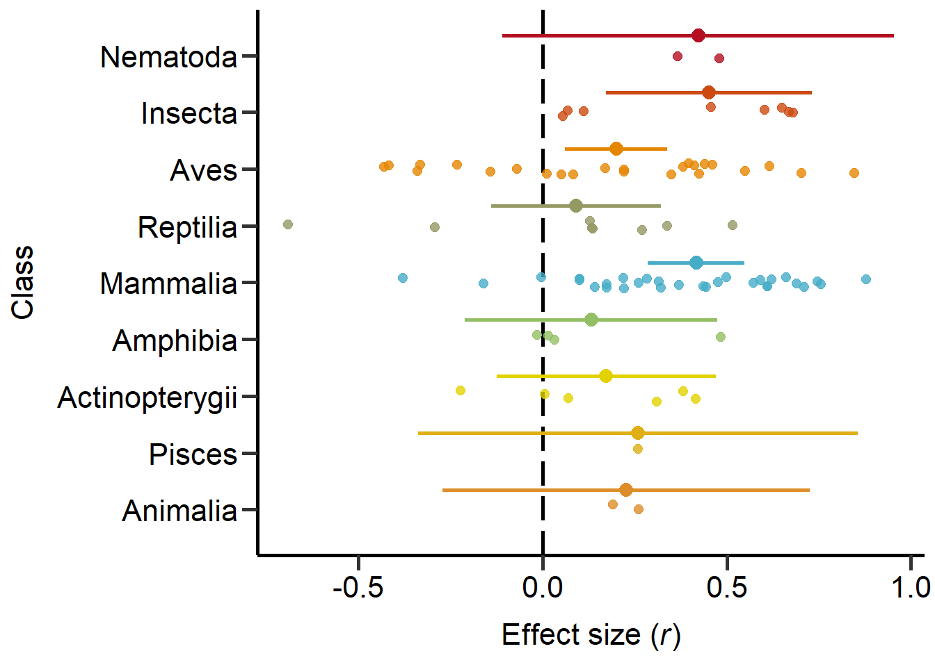

Figure 3: Phylogeny based on classes including sample sizes for the number of studies and number of effect sizes, respectively, and estimates with 95%CI from non-phylogenetic model.

Type of SSD measure

Next we explored the effect of the type of SSD measure (i.e. body mass or size):

MetaData$SSD_Proxy=as.factor(MetaData$SSD_Proxy)
MetaData$SSD_Proxy=relevel(MetaData$SSD_Proxy,c("Body mass"))
Model_REML_by_cSSDMeasure = rma.mv(r ~ SSD_Proxy, V=Var_r, data = MetaData, random = c(~ 1 | Study_ID,~ 1 | Index), method = "REML")
summary(Model_REML_by_cSSDMeasure)


Multivariate Meta-Analysis Model (k = 83; method: REML)

  logLik  Deviance       AIC       BIC      AICc   
-24.2720   48.5441   56.5441   66.1219   57.0704   

Variance Components:

            estim    sqrt  nlvls  fixed    factor 
sigma^2.1  0.0316  0.1777     50     no  Study_ID 
sigma^2.2  0.0635  0.2521     83     no     Index 

Test for Residual Heterogeneity:
QE(df = 81) = 1404.5159, p-val < .0001

Test of Moderators (coefficient 2):
QM(df = 1) = 2.1342, p-val = 0.1440

Model Results:

                    estimate      se     zval    pval    ci.lb   ci.ub      
intrcpt               0.3542  0.0626   5.6615  <.0001   0.2316  0.4768  *** 
SSD_ProxyBody size   -0.1196  0.0818  -1.4609  0.1440  -0.2800  0.0408      

---
Signif. codes:  0 '***' 0.001 '**' 0.01 '*' 0.05 '.' 0.1 ' ' 1

We then re-leveled the model for post-hoc comparisons:

MetaData$SSD_Proxy=relevel(MetaData$SSD_Proxy,c("Body size"))
Model_REML_by_cSSDMeasure2 = rma.mv(r ~ SSD_Proxy, V=Var_r, data = MetaData, random = c(~ 1 | Study_ID,~ 1 | Index), method = "REML")
summary(Model_REML_by_cSSDMeasure2)

Finally, we computed FDR corrected p-values:

tab3=as.data.frame(round(p.adjust(c(.0001, .0001), method = 'fdr'),digit=3),row.names=cbind("Body mass","Body size"))
colnames(tab3)<-cbind('P-value')
tab3

          P-value
Body mass       0
Body size       0

SSD measure controlled for body size?

Next we explored the effect if the primary study controlled the SSD for body size (i.e. uncontrolled or controlled):

MetaData$BodySizeControlled=as.factor(MetaData$BodySizeControlled)
MetaData$BodySizeControlled=relevel(MetaData$BodySizeControlled,c("No"))
Model_REML_by_cBodySizeCont = rma.mv(r ~ BodySizeControlled, V=Var_r, data = MetaData, random = c(~ 1 | Study_ID,~ 1 | Index), method = "REML")
summary(Model_REML_by_cBodySizeCont)


Multivariate Meta-Analysis Model (k = 85; method: REML)

  logLik  Deviance       AIC       BIC      AICc   
-24.7551   49.5102   57.5102   67.1855   58.0230   

Variance Components:

            estim    sqrt  nlvls  fixed    factor 
sigma^2.1  0.0334  0.1828     51     no  Study_ID 
sigma^2.2  0.0626  0.2502     85     no     Index 

Test for Residual Heterogeneity:
QE(df = 83) = 1445.3959, p-val < .0001

Test of Moderators (coefficient 2):
QM(df = 1) = 0.6106, p-val = 0.4346

Model Results:

                       estimate      se     zval    pval    ci.lb   ci.ub      
intrcpt                  0.2983  0.0459   6.4948  <.0001   0.2083  0.3883  *** 
BodySizeControlledYes   -0.0799  0.1023  -0.7814  0.4346  -0.2804  0.1205      

---
Signif. codes:  0 '***' 0.001 '**' 0.01 '*' 0.05 '.' 0.1 ' ' 1

We then re-leveled the model for post-hoc comparisons:

MetaData$BodySizeControlled=relevel(MetaData$BodySizeControlled,c("Yes"))
Model_REML_by_cBodySizeCont2 = rma.mv(r ~ BodySizeControlled, V=Var_r, data = MetaData, random = c(~ 1 | Study_ID,~ 1 | Index), method = "REML")
summary(Model_REML_by_cBodySizeCont2)

Finally, we computed FDR corrected p-values:

tab4=as.data.frame(round(p.adjust(c(.0001, 0.0168), method = 'fdr'),digit=3),row.names=cbind("uncontrolled","controlled"))
colnames(tab4)<-cbind('P-value')
tab4

             P-value
uncontrolled   0.000
controlled     0.017

Phylogentic vs non-phylogenetic studies

Next we explored the effect of studies controlling for phylogeny vs non-phylogenetic studies:

MetaData$PhyloControlled=as.factor(MetaData$PhyloControlled)
MetaData$PhyloControlled=relevel(MetaData$PhyloControlled,c("No"))
Model_cREML_by_cPhylo = rma.mv(r ~ PhyloControlled, V=Var_r, data = MetaData, random = c(~ 1 | Study_ID,~ 1 | Index), method = "REML")
summary(Model_cREML_by_cPhylo)


Multivariate Meta-Analysis Model (k = 85; method: REML)

  logLik  Deviance       AIC       BIC      AICc   
-21.6552   43.3104   51.3104   60.9858   51.8232   

Variance Components:

            estim    sqrt  nlvls  fixed    factor 
sigma^2.1  0.0157  0.1252     51     no  Study_ID 
sigma^2.2  0.0698  0.2642     85     no     Index 

Test for Residual Heterogeneity:
QE(df = 83) = 1214.8661, p-val < .0001

Test of Moderators (coefficient 2):
QM(df = 1) = 7.8737, p-val = 0.0050

Model Results:

                    estimate      se     zval    pval    ci.lb    ci.ub      
intrcpt               0.5883  0.1176   5.0034  <.0001   0.3578   0.8187  *** 
PhyloControlledYes   -0.3478  0.1240  -2.8060  0.0050  -0.5908  -0.1049   ** 

---
Signif. codes:  0 '***' 0.001 '**' 0.01 '*' 0.05 '.' 0.1 ' ' 1

We then re-leveled the model for post-hoc comparisons:

MetaData$PhyloControlled=relevel(MetaData$PhyloControlled,c("Yes"))
Model_cREML_by_cPhylo2 = rma.mv(r ~ PhyloControlled, V=Var_r, data = MetaData, random = c(~ 1 | Study_ID,~ 1 | Index), method = "REML")
summary(Model_cREML_by_cPhylo2)

Finally, we computed FDR corrected p-values:

tab5=as.data.frame(round(p.adjust(c(0.0001, 0.0001), method = 'fdr'),digit=3),row.names=cbind("Non-phylogenetic","With phylogeny"))
colnames(tab5)<-cbind('P-value')
tab5

                 P-value
Non-phylogenetic       0
With phylogeny         0

Test for publication bias

Model_cREML_PublBias         = rma.mv(z ~ SE_z, V=rep(((mean(SE_z)*mean(SE_z))*N),length(SE_z)), data = MetaData, random = c(~ 1 | Study_ID,~ 1 | Index), method = "REML")
summary(Model_cREML_PublBias)


Multivariate Meta-Analysis Model (k = 85; method: REML)

   logLik   Deviance        AIC        BIC       AICc   
-101.0851   202.1703   210.1703   219.8456   210.6831   

Variance Components:

            estim    sqrt  nlvls  fixed    factor 
sigma^2.1  0.0000  0.0000     51     no  Study_ID 
sigma^2.2  0.0000  0.0000     85     no     Index 

Test for Residual Heterogeneity:
QE(df = 83) = 14.4691, p-val = 1.0000

Test of Moderators (coefficient 2):
QM(df = 1) = 2.8672, p-val = 0.0904

Model Results:

         estimate      se    zval    pval    ci.lb   ci.ub    
intrcpt    0.0674  0.2533  0.2663  0.7900  -0.4290  0.5638    
SE_z       1.5228  0.8993  1.6933  0.0904  -0.2398  3.2854  . 

---
Signif. codes:  0 '***' 0.001 '**' 0.01 '*' 0.05 '.' 0.1 ' ' 1

Publication year

Next we explored the effect of the publication year of each study:

Model_cREML_by_Year = rma.mv(r ~ Year, V=Var_r, data = MetaData, random = c(~ 1 | Study_ID,~ 1 | Index), method = "REML")
summary(Model_cREML_by_Year)


Multivariate Meta-Analysis Model (k = 85; method: REML)

  logLik  Deviance       AIC       BIC      AICc   
-23.2555   46.5110   54.5110   64.1863   55.0238   

Variance Components:

            estim    sqrt  nlvls  fixed    factor 
sigma^2.1  0.0293  0.1712     51     no  Study_ID 
sigma^2.2  0.0617  0.2484     85     no     Index 

Test for Residual Heterogeneity:
QE(df = 83) = 1136.4440, p-val < .0001

Test of Moderators (coefficient 2):
QM(df = 1) = 3.7310, p-val = 0.0534

Model Results:

         estimate      se     zval    pval    ci.lb    ci.ub    
intrcpt   15.0587  7.6506   1.9683  0.0490   0.0639  30.0535  * 
Year      -0.0074  0.0038  -1.9316  0.0534  -0.0148   0.0001  . 

---
Signif. codes:  0 '***' 0.001 '**' 0.01 '*' 0.05 '.' 0.1 ' ' 1

Forest plot

# Sort data by Class
MetaData$Class=as.factor(MetaData$Class)
MetaData$Class=factor(MetaData$Class, levels = c("Animalia","Pisces" ,"Actinopterygii","Amphibia","Mammalia","Reptilia","Aves","Insecta","Nematoda"))
MetaData_sorted <-MetaData[order(MetaData$Class),]

# Add global effect size to data
forestData=MetaData_sorted[,c(3,5,12,17,20,21)]
GlobalES=as.data.frame(cbind('Global effect size','','Global effect size',Model_REML_Null$b[1,1],Model_REML_Null$ci.lb[1],Model_REML_Null$ci.ub[1]))
colnames(GlobalES)=c('AuthorsAndYear','Class','SexSel_Mode','r','lCI','uCI')
forestData=rbind(GlobalES,forestData)
forestData[,c(4:6)]=lapply(forestData[,c(4:6)],as.numeric)
forestData$SexSel_Mode=as.factor(forestData$SexSel_Mode)
forestData$SexSel_Mode=factor(forestData$SexSel_Mode, levels = c("pre-copulatory","post-copulatory" ,"both","Global effect size"))

Figure 1

ggplot(data=forestData, aes(y=1:nrow(forestData), x=r, xmin=lCI, xmax=uCI,color=SexSel_Mode)) +
  geom_vline(xintercept=0, color='black', linetype='dashed', alpha=.5,linewidth=0.8) +
  geom_point(size = ifelse(1:nrow(forestData) == c(1), 2.75, 1.8))+
  geom_errorbarh(height=0,size = ifelse(1:nrow(forestData) == c(1), 1.25, 1))+
  scale_y_continuous(breaks=seq(1, nrow(forestData), by=1), labels=forestData$AuthorsAndYear,limits=c(1,length(forestData$AuthorsAndYear)),expand=c(0.015,0.015)) +
  labs(title='', x=expression(paste(italic("r "),'(95% CI)')), y = 'Study') +
  theme_classic()+theme(axis.text.x=element_text(size=12),
                        axis.title=element_text(size=12))+ labs(color =  c("Sexual selection mode"))+ 
  scale_colour_manual(values=Meta_col, labels=c('Pre-copulatory','Post-copulatory',"Both","Global effect size"))+
  guides(color = guide_legend(override.aes = list(size = .9)))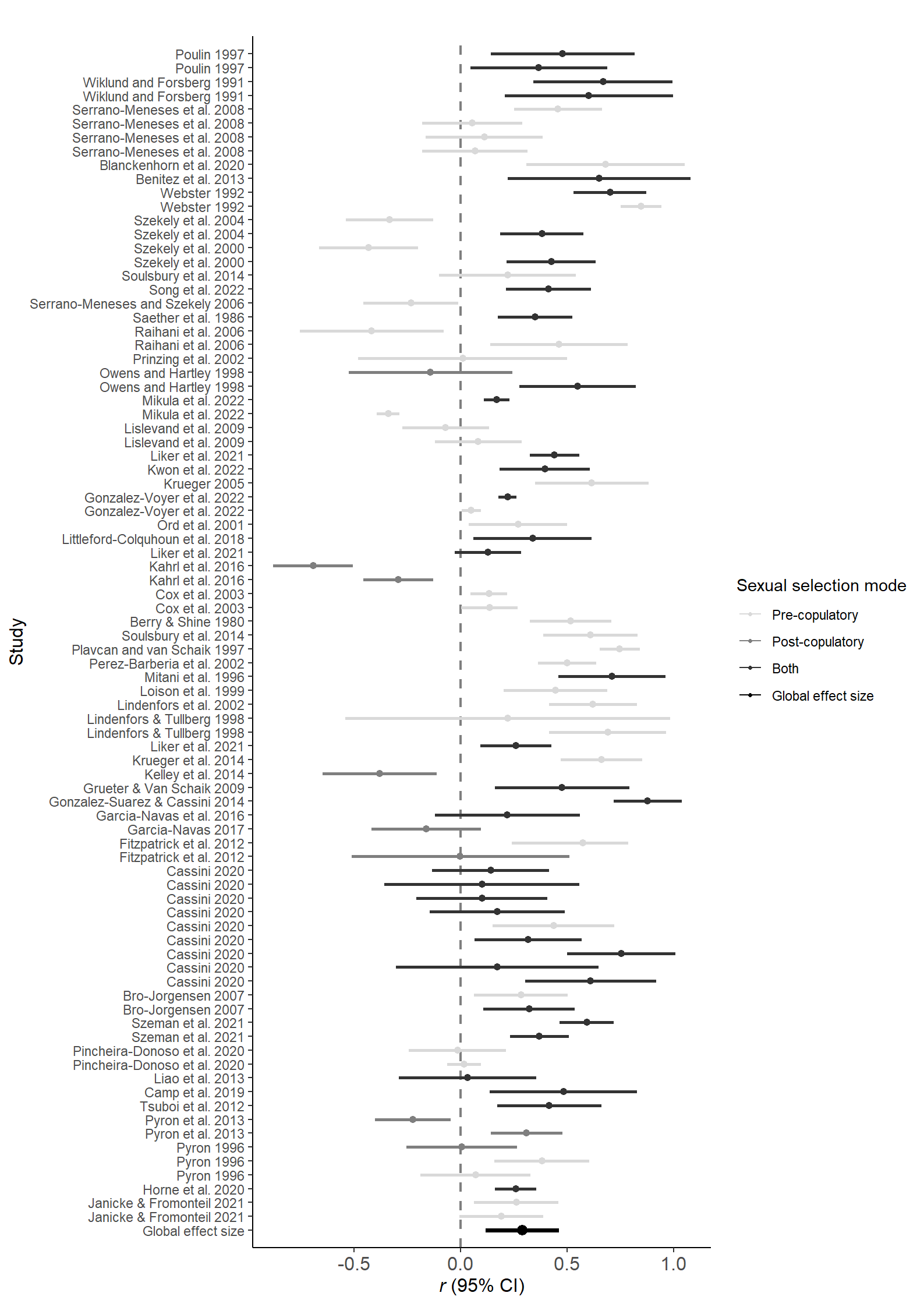

Figure 1: Forest plot including correlation coefficients (±95% CI), as well as the global effect size (in grey) with and without controlling for phylogeny. Different animal classes highlighted by background colors (see Figure 3 for class names) and sexual selection modes pre- (red), post-copulatory (blue) and both (green) by color of effect size.

sessionInfo()

R version 4.2.3 (2023-03-15 ucrt)
Platform: x86_64-w64-mingw32/x64 (64-bit)
Running under: Windows 10 x64 (build 19045)

Matrix products: default

locale:
[1] LC_COLLATE=German_Germany.utf8  LC_CTYPE=German_Germany.utf8   
[3] LC_MONETARY=German_Germany.utf8 LC_NUMERIC=C                   
[5] LC_TIME=German_Germany.utf8    

attached base packages:
[1] stats     graphics  grDevices utils     datasets  methods   base     

other attached packages:
 [1] wesanderson_0.3.6   PupillometryR_0.0.4 rlang_1.1.0        
 [4] dplyr_1.1.1         cowplot_1.1.1       ggdist_3.3.0       
 [7] MCMCglmm_2.34       coda_0.19-4         RColorBrewer_1.1-3 
[10] ggplot2_3.4.2       data.table_1.14.8   multcomp_1.4-23    
[13] TH.data_1.1-2       survival_3.5-3      mvtnorm_1.1-3      
[16] psych_2.3.3         pwr_1.3-0           MASS_7.3-58.2      
[19] metafor_4.2-0       numDeriv_2016.8-1.1 metadat_1.2-0      
[22] Matrix_1.5-3        matrixcalc_1.0-6    ape_5.7-1          
[25] workflowr_1.7.0    

loaded via a namespace (and not attached):
 [1] httr_1.4.5           sass_0.4.5           jsonlite_1.8.4      
 [4] splines_4.2.3        bslib_0.4.2          getPass_0.2-2       
 [7] distributional_0.3.2 highr_0.10           tensorA_0.36.2      
[10] yaml_2.3.7           pillar_1.9.0         lattice_0.20-45     
[13] glue_1.6.2           digest_0.6.31        promises_1.2.0.1    
[16] colorspace_2.1-0     sandwich_3.0-2       htmltools_0.5.5     
[19] httpuv_1.6.9         pkgconfig_2.0.3      corpcor_1.6.10      
[22] scales_1.2.1         processx_3.8.0       whisker_0.4.1       
[25] later_1.3.0          cubature_2.0.4.6     git2r_0.31.0        
[28] tibble_3.2.1         generics_0.1.3       farver_2.1.1        
[31] cachem_1.0.7         withr_2.5.0          cli_3.6.1           
[34] mnormt_2.1.1         magrittr_2.0.3       evaluate_0.20       
[37] ps_1.7.3             fs_1.6.1             fansi_1.0.4         
[40] nlme_3.1-162         tools_4.2.3          lifecycle_1.0.3     
[43] stringr_1.5.0        munsell_0.5.0        callr_3.7.3         
[46] compiler_4.2.3       jquerylib_0.1.4      grid_4.2.3          
[49] rstudioapi_0.14      labeling_0.4.2       rmarkdown_2.21      
[52] gtable_0.3.3         codetools_0.2-19     R6_2.5.1            
[55] zoo_1.8-12           knitr_1.42           fastmap_1.1.1       
[58] utf8_1.2.3           mathjaxr_1.6-0       rprojroot_2.0.3     
[61] stringi_1.7.12       parallel_4.2.3       Rcpp_1.0.10         
[64] vctrs_0.6.1          tidyselect_1.2.0     xfun_0.38