Global model Version 1

Global models Version 2

Moderator tests for phylogenetic models

Sexual selection mode
Plot sexual selection mode (Figure 2)
Sexual selection category
Plot sexual selection category (Figure S1)
Type of SSD measure
Plot Type of SSD measure (Figure S2A)
SSD measure controlled for body size?
Plot: SSD measure controlled for body size? (Figure S2B)
Test for publication bias
Figure S2D
Publication year
Plot publication year (Figure S2E)

Moderator tests for non-phylogenetic models

Sexual selection mode
Sexual selection category
Phylogenetic classes
Plot phylogenetic classes (Figure 3)
Type of SSD measure
SSD measure controlled for body size?
Test for publication bias
Publication year

Forest plot

Figure 1

Sexual selection and sexual size dimorphism: a meta-analysis of comparative studies

Additional analyses

Lennart Winkler¹, Robert P Freckleton², Tamas Szekely³, ⁴ & Tim Janicke^1,5

¹Applied Zoology, Technical University Dresden

²Department of Zoology, University of Oxford, South Parks Road, Oxford OX1 3PS, UK

³Milner Centre for Evolution, University of Bath, Bath, UK8

⁴Department of Evolutionary Zoology and Human Behaviour, University of Debrecen, Debrecen, Hungary

⁵Centre d’Écologie Fonctionnelle et Évolutive, UMR 5175, CNRS, Université de Montpellier

Last updated: 2023-05-24

Checks: 7 0

Knit directory: SSD_and_sexual_selection_2023/

This reproducible R Markdown analysis was created with workflowr (version 1.7.0). The Checks tab describes the reproducibility checks that were applied when the results were created. The Past versions tab lists the development history.

R Markdown file: up-to-date

Great! Since the R Markdown file has been committed to the Git repository, you know the exact version of the code that produced these results.

Environment: empty

Great job! The global environment was empty. Objects defined in the global environment can affect the analysis in your R Markdown file in unknown ways. For reproduciblity it’s best to always run the code in an empty environment.

Seed: set.seed(20230430)

The command set.seed(20230430) was run prior to running the code in the R Markdown file. Setting a seed ensures that any results that rely on randomness, e.g. subsampling or permutations, are reproducible.

Session information: recorded

Great job! Recording the operating system, R version, and package versions is critical for reproducibility.

Cache: none

Nice! There were no cached chunks for this analysis, so you can be confident that you successfully produced the results during this run.

File paths: relative

Great job! Using relative paths to the files within your workflowr project makes it easier to run your code on other machines.

Repository version: c1d3311

Great! You are using Git for version control. Tracking code development and connecting the code version to the results is critical for reproducibility.

The results in this page were generated with repository version c1d3311. See the Past versions tab to see a history of the changes made to the R Markdown and HTML files.

Note that you need to be careful to ensure that all relevant files for the analysis have been committed to Git prior to generating the results (you can use wflow_publish or wflow_git_commit). workflowr only checks the R Markdown file, but you know if there are other scripts or data files that it depends on. Below is the status of the Git repository when the results were generated:


Ignored files:
    Ignored:    .Rhistory

Note that any generated files, e.g. HTML, png, CSS, etc., are not included in this status report because it is ok for generated content to have uncommitted changes.

These are the previous versions of the repository in which changes were made to the R Markdown (analysis/index2.Rmd) and HTML (docs/index2.html) files. If you’ve configured a remote Git repository (see ?wflow_git_remote), click on the hyperlinks in the table below to view the files as they were in that past version.

File	Version	Author	Date	Message
Rmd	c1d3311	LennartWinkler	2023-05-24	wflow_publish(all = T)
html	71d667c	LennartWinkler	2023-05-03	Build site.
Rmd	378a58c	LennartWinkler	2023-05-03	wflow_publish(republish = TRUE, all = T)
html	085f45f	LennartWinkler	2023-05-03	Build site.
Rmd	9c4346c	LennartWinkler	2023-05-03	wflow_publish(republish = TRUE, all = T)
html	9c4346c	LennartWinkler	2023-05-03	wflow_publish(republish = TRUE, all = T)
Rmd	85c143e	LennartWinkler	2023-05-03	update
html	8edd942	LennartWinkler	2023-05-01	Build site.
Rmd	d131cd9	LennartWinkler	2023-05-01	wflow_publish(republish = TRUE, all = T)
Rmd	57ca562	LennartWinkler	2023-04-30	update
html	57ca562	LennartWinkler	2023-04-30	update
Rmd	7a0f67c	LennartWinkler	2023-04-30	Set up project

Supplementary material reporting R code for the manuscript ‘Sexual selection and sexual size dimorphism: a meta-analysis of comparative studies’.
Additional analyses excluding studies that did not correct for phylogenetic non-independence (see Supplement 2). # Load and prepare data Before we started the analyses, we loaded all necessary packages and data.

rm(list = ls()) # Clear work environment

# Load R-packages ####
list_of_packages=cbind('ape','matrixcalc','metafor','Matrix','MASS','pwr','psych','multcomp','data.table','ggplot2','RColorBrewer','MCMCglmm','ggdist','cowplot','PupillometryR','dplyr','wesanderson')
lapply(list_of_packages, require, character.only = TRUE)

# Load data set ####
MetaData <- read.csv("./data/Supplement4_SexSelSSD_V01.csv", sep=";", header=TRUE) # Load data set

#Remove studies that did not correct for phylogenetic non-independence
MetaData=MetaData[MetaData$PhyloControlled=='Yes',]

N_Studies <- length(summary(as.factor(MetaData$Study_ID))) # Number of included primary studies

Tree<- read.tree("./data/Supplement6_SexSelSSD_V01.txt") # Load phylogenetic tree

# Prune phylogenetic tree
MetaData_Class_Data <- unique(MetaData$Class)
Tree_Class<-drop.tip(Tree, Tree$tip.label[-na.omit(match(MetaData_Class_Data, Tree$tip.label))])
forcedC_Moderators <- as.matrix(forceSymmetric(vcv(Tree_Class, corr=TRUE)))

# Order moderator levels
MetaData$SexSel_Mode=as.factor(MetaData$SexSel_Mode)
MetaData$SexSel_Mode=relevel(MetaData$SexSel_Mode,c("post-copulatory"))
MetaData$SexSel_Mode=relevel(MetaData$SexSel_Mode,c("pre-copulatory"))
MetaData$SexSel_Sex=as.factor(MetaData$SexSel_Sex)
MetaData$SexSel_Sex=relevel(MetaData$SexSel_Sex,c("Male"))

# Set figure theme and colors
theme=theme(panel.border = element_blank(), 
            panel.background = element_blank(),
            panel.grid.major = element_blank(),
            panel.grid.minor = element_blank(), 
            legend.position = c(0.2,0.5),
            legend.title = element_blank(),
            legend.text = element_text(colour="black", size=12),
            axis.line.x = element_line(colour = "black", size = 1),
            axis.line.y = element_line(colour = "black", size = 1),
            axis.text.x = element_text(face="plain", color="black", size=16, angle=0),
            axis.text.y = element_text(face="plain", color="black", size=16, angle=0),
            axis.title.x = element_text(size=16,face="plain", margin = margin(r=0,10,0,0)),
            axis.title.y = element_text(size=16,face="plain", margin = margin(r=10,0,0,0)),
            axis.ticks = element_line(size = 1),
            axis.ticks.length = unit(.3, "cm"))

colpal=c("#4DAF4A","#377EB8","#E41A1C")
colpal2=brewer.pal(7, 'Dark2')
colpal3=wes_palette('FantasticFox1', 9, type = c("continuous"))
colpal4=c("grey50","grey65")
Meta_col=c('grey85','grey50','grey20','black')

# Global models ####

# Phylogenetic Model
Model_REML_Null         = rma.mv(r ~ 1, V=Var_r, data = MetaData, random = c(~ 1 | Study_ID,~ 1 | Index, ~ 1 | Class), R = list(Class = forcedC_Moderators), method = "REML")
summary(Model_REML_Null)

# Non-phylogenetic Model
Model_cREML_Null         = rma.mv(r ~ 1, V=Var_r, data = MetaData, random = c(~ 1 | Study_ID,~ 1 | Index), method = "REML")
summary(Model_cREML_Null)

Global model Version 1

First, we tested if increasing sexual selection (estimated via diverse proxies; see Table S1) correlated with the degree of SSD. To this end we ran a global model on the absolute correlation coefficients extracted from primary studies (i.e. increasing sexual selection could correlate with a female- or male-bias in SSD, with all resulting correlation coefficients being positive).

First, we ran a global model including the phylogeny:

# Set all correlation coeficients as positive
MetaData$absSSDcor=NA
MetaData$absSSDcor=abs(MetaData$r)
# Phylogenetic Model
Model_REML_Null         = rma.mv(absSSDcor ~ 1, V=Var_r, data = MetaData, random = c(~ 1 | Study_ID,~ 1 | Index, ~ 1 | Class), R = list(Class = forcedC_Moderators), method = "REML")
summary(Model_REML_Null)


Multivariate Meta-Analysis Model (k = 77; method: REML)

  logLik  Deviance       AIC       BIC      AICc   
 10.3881  -20.7762  -12.7762   -3.4533  -12.2128   

Variance Components:

            estim    sqrt  nlvls  fixed    factor    R 
sigma^2.1  0.0092  0.0958     45     no  Study_ID   no 
sigma^2.2  0.0178  0.1334     77     no     Index   no 
sigma^2.3  0.0132  0.1149      9     no     Class  yes 

Test for Heterogeneity:
Q(df = 76) = 545.0814, p-val < .0001

Model Results:

estimate      se    zval    pval   ci.lb   ci.ub      
  0.3032  0.0722  4.1998  <.0001  0.1617  0.4447  *** 

---
Signif. codes:  0 '***' 0.001 '**' 0.01 '*' 0.05 '.' 0.1 ' ' 1

Second, we ran a global model without the phylogeny:

# Non-phylogenetic Model
Model_cREML_Null         = rma.mv(absSSDcor ~ 1, V=Var_r, data = MetaData, random = c(~ 1 | Study_ID,~ 1 | Index), method = "REML")
summary(Model_cREML_Null)


Multivariate Meta-Analysis Model (k = 77; method: REML)

  logLik  Deviance       AIC       BIC      AICc   
  8.0489  -16.0978  -10.0978   -3.1056   -9.7645   

Variance Components:

            estim    sqrt  nlvls  fixed    factor 
sigma^2.1  0.0153  0.1236     45     no  Study_ID 
sigma^2.2  0.0198  0.1409     77     no     Index 

Test for Heterogeneity:
Q(df = 76) = 545.0814, p-val < .0001

Model Results:

estimate      se     zval    pval   ci.lb   ci.ub      
  0.3547  0.0290  12.2423  <.0001  0.2979  0.4115  *** 

---
Signif. codes:  0 '***' 0.001 '**' 0.01 '*' 0.05 '.' 0.1 ' ' 1

Global models Version 2

Next, we addressed the question if increasing sexual selection correlated with an increasingly male-biased SSD. For this we ran a global model including an observation-level index and the study identifier as random termson correlation coefficients that were positive if increasing sexual selection correlated with an increasingly male-biased SSD, but negative if increasing sexual selection correlated with an increasingly female-biased SSD.

First, we ran a global model including the phylogeny:

Model_REML_Null         = rma.mv(r ~ 1, V=Var_r, data = MetaData, random = c(~ 1 | Study_ID,~ 1 | Index, ~ 1 | Class), R = list(Class = forcedC_Moderators), method = "REML")
summary(Model_REML_Null)


Multivariate Meta-Analysis Model (k = 77; method: REML)

  logLik  Deviance       AIC       BIC      AICc   
-19.6871   39.3743   47.3743   56.6972   47.9377   

Variance Components:

            estim    sqrt  nlvls  fixed    factor    R 
sigma^2.1  0.0000  0.0000     45     no  Study_ID   no 
sigma^2.2  0.0757  0.2751     77     no     Index   no 
sigma^2.3  0.0237  0.1539      9     no     Class  yes 

Test for Heterogeneity:
Q(df = 76) = 1182.7000, p-val < .0001

Model Results:

estimate      se    zval    pval   ci.lb   ci.ub    
  0.2341  0.0963  2.4321  0.0150  0.0455  0.4228  * 

---
Signif. codes:  0 '***' 0.001 '**' 0.01 '*' 0.05 '.' 0.1 ' ' 1

Second, we ran a global model without the phylogeny:

Model_cREML_Null         = rma.mv(r ~ 1, V=Var_r, data = MetaData, random = c(~ 1 | Study_ID,~ 1 | Index), method = "REML")
summary(Model_cREML_Null)


Multivariate Meta-Analysis Model (k = 77; method: REML)

  logLik  Deviance       AIC       BIC      AICc   
-22.2286   44.4572   50.4572   57.4494   50.7905   

Variance Components:

            estim    sqrt  nlvls  fixed    factor 
sigma^2.1  0.0143  0.1195     45     no  Study_ID 
sigma^2.2  0.0772  0.2778     77     no     Index 

Test for Heterogeneity:
Q(df = 76) = 1182.7000, p-val < .0001

Model Results:

estimate      se    zval    pval   ci.lb   ci.ub      
  0.2393  0.0401  5.9736  <.0001  0.1608  0.3178  *** 

---
Signif. codes:  0 '***' 0.001 '**' 0.01 '*' 0.05 '.' 0.1 ' ' 1

Moderator tests for phylogenetic models

Next, we ran a series of models that test the effect of different moderators.
Again we started with models including the phylogeny.

Sexual selection mode

The first model explores the effect of the sexual selection mode (i.e. pre-copulatory, post-copulatory or both):

MetaData$SexSel_Mode=relevel(MetaData$SexSel_Mode,c("pre-copulatory"))
Model_REML_by_SexSelMode = rma.mv(r ~ factor(SexSel_Mode), V=Var_r, data = MetaData, random = c(~ 1 | Study_ID,~ 1 | Index, ~ 1 | Class), R = list(Class = forcedC_Moderators), method = "REML")
summary(Model_REML_by_SexSelMode)


Multivariate Meta-Analysis Model (k = 77; method: REML)

  logLik  Deviance       AIC       BIC      AICc   
 -7.6879   15.3757   27.3757   41.2001   28.6294   

Variance Components:

            estim    sqrt  nlvls  fixed    factor    R 
sigma^2.1  0.0013  0.0361     45     no  Study_ID   no 
sigma^2.2  0.0489  0.2212     77     no     Index   no 
sigma^2.3  0.0231  0.1519      9     no     Class  yes 

Test for Residual Heterogeneity:
QE(df = 74) = 944.4229, p-val < .0001

Test of Moderators (coefficients 2:3):
QM(df = 2) = 30.0173, p-val < .0001

Model Results:

                                    estimate      se     zval    pval    ci.lb 
intrcpt                               0.2305  0.0954   2.4172  0.0156   0.0436 
factor(SexSel_Mode)post-copulatory   -0.4418  0.1035  -4.2669  <.0001  -0.6447 
factor(SexSel_Mode)both               0.1330  0.0653   2.0381  0.0415   0.0051 
                                      ci.ub      
intrcpt                              0.4174    * 
factor(SexSel_Mode)post-copulatory  -0.2388  *** 
factor(SexSel_Mode)both              0.2610    * 

---
Signif. codes:  0 '***' 0.001 '**' 0.01 '*' 0.05 '.' 0.1 ' ' 1

We then re-leveled the model for post-hoc comparisons:

MetaData$SexSel_Mode=relevel(MetaData$SexSel_Mode,c("post-copulatory"))
Model_REML_by_SexSelMode2 = rma.mv(r ~ factor(SexSel_Mode), V=Var_r, data = MetaData, random = c(~ 1 | Study_ID,~ 1 | Index, ~ 1 | Class), R = list(Class = forcedC_Moderators), method = "REML")
summary(Model_REML_by_SexSelMode2)

MetaData$SexSel_Mode=relevel(MetaData$SexSel_Mode,c("both"))
Model_REML_by_SexSelMode3 = rma.mv(r ~ factor(SexSel_Mode), V=Var_r, data = MetaData, random = c(~ 1 | Study_ID,~ 1 | Index, ~ 1 | Class), R = list(Class = forcedC_Moderators), method = "REML")
summary(Model_REML_by_SexSelMode3)

Finally, we computed FDR corrected p-values:

tab1=as.data.frame(round(p.adjust(c(0.0029, 0.1203, .0001), method = 'fdr'),digit=3),row.names=cbind("Pre-copulatory","Post-copulatory","Both"))
colnames(tab1)<-cbind('P-value')
tab1

                P-value
Pre-copulatory    0.004
Post-copulatory   0.120
Both              0.000

Plot sexual selection mode (Figure 2)

Here we plot the sexual selection mode moderator:

MetaData$SexSel_Mode=factor(MetaData$SexSel_Mode, levels = c("both","post-copulatory" ,"pre-copulatory"))

ggplot(MetaData, aes(x=SexSel_Mode, y=r, fill = SexSel_Mode, colour = SexSel_Mode)) +
  geom_hline(yintercept=0, linetype="longdash", color = "black", linewidth=1)+
  geom_flat_violin(position = position_nudge(x = 0.25, y = 0),adjust =1, trim = F,alpha=0.6)+
  geom_point(position = position_jitter(width = .1), size = 2.5,alpha=0.6,stroke=0,shape=19)+
  geom_point(inherit.aes = F,mapping = aes(y=Model_REML_by_SexSelMode$b[1,1], x=3.25), size = 3.5,alpha=1,stroke=0,shape=19,color='grey30')+
  geom_point(inherit.aes = F,mapping = aes(y=Model_REML_by_SexSelMode2$b[1,1], x=2.25), size = 3.5,alpha=1,stroke=0,shape=19,color='grey30')+
  geom_point(inherit.aes = F,mapping = aes(y=Model_REML_by_SexSelMode3$b[1,1], x=1.25), size = 3.5,alpha=1,stroke=0,shape=19,color='grey30')+
  geom_segment(inherit.aes = F,mapping = aes(y=Model_REML_by_SexSelMode$ci.lb[1], x=3.25, xend= 3.25, yend= Model_REML_by_SexSelMode$ci.ub[1]), alpha=1,linewidth=1,color='grey30')+
  geom_segment(inherit.aes = F,mapping = aes(y=Model_REML_by_SexSelMode2$ci.lb[1], x=2.25, xend= 2.25, yend= Model_REML_by_SexSelMode2$ci.ub[1]), alpha=1,linewidth=1,color='grey30')+
  geom_segment(inherit.aes = F,mapping = aes(y=Model_REML_by_SexSelMode3$ci.lb[1], x=1.25, xend= 1.25, yend= Model_REML_by_SexSelMode3$ci.ub[1]), alpha=1,linewidth=1,color='grey30')+
  ylab(expression(paste("Effect size (", italic("r"),')')))+xlab('Sexual selection mode')+coord_flip()+guides(fill = FALSE, colour = FALSE) +
  scale_color_manual(values =colpal)+
  scale_fill_manual(values =colpal)+
  scale_x_discrete(labels=c("Both","Post-copulatory" ,"Pre-copulatory"),expand=c(.1,0))+
  annotate("text", x=1, y=1.2, label= "n = 37",size=4.5) +
  annotate("text", x=2, y=1.2, label= "n = 9",size=4.5) +
  annotate("text", x=3, y=1.2, label= "n = 39",size=4.5) + theme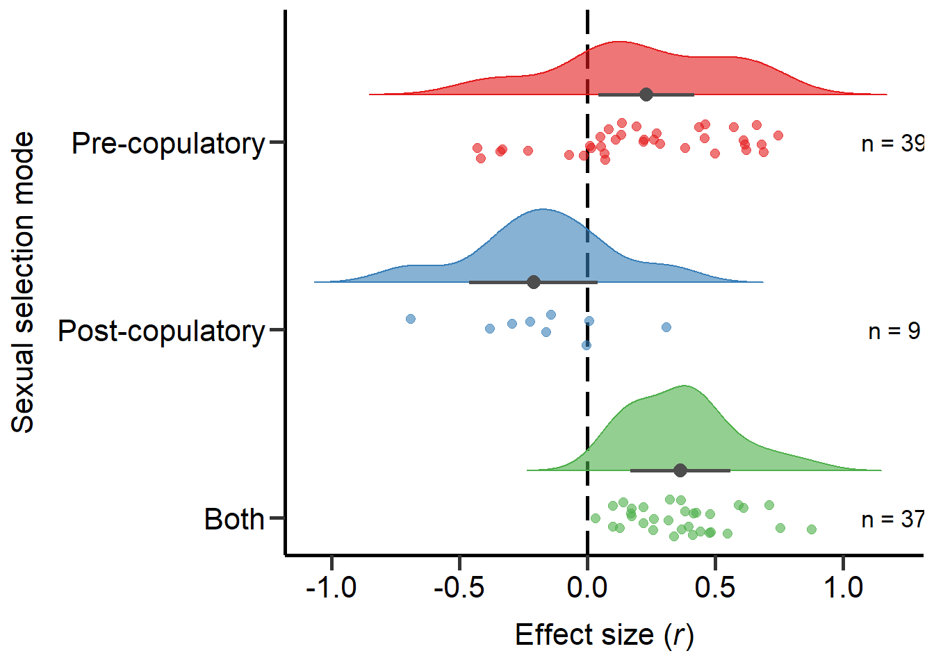

Figure 2: Raincloud plot of correlation coefficients between SSD and the modes of sexual selection proxies (i.e. pre-copulatory, post-copulatory or both) including sample sizes and estimates with 95%CI from phylogenetic model.

Sexual selection category

Next we explored the effect of the sexual selection category (i.e. density, mating system, operational sex ratio (OSR), post-mating competition, pre-mating competition, trait-based, other):

MetaData$SexSel_Category=as.factor(MetaData$SexSel_Category)
MetaData$SexSel_Category=relevel(MetaData$SexSel_Category,c("Postmating competition"))
Model_REML_by_SexSelCat = rma.mv(r ~ factor(SexSel_Category), V=Var_r, data = MetaData, random = c(~ 1 | Study_ID,~ 1 | Index, ~ 1 | Class), R = list(Class = forcedC_Moderators), method = "REML")
summary(Model_REML_by_SexSelCat)


Multivariate Meta-Analysis Model (k = 77; method: REML)

  logLik  Deviance       AIC       BIC      AICc   
  1.5992   -3.1985   16.8015   39.2865   20.5304   

Variance Components:

            estim    sqrt  nlvls  fixed    factor    R 
sigma^2.1  0.0099  0.0995     45     no  Study_ID   no 
sigma^2.2  0.0280  0.1674     77     no     Index   no 
sigma^2.3  0.0211  0.1452      9     no     Class  yes 

Test for Residual Heterogeneity:
QE(df = 70) = 614.1683, p-val < .0001

Test of Moderators (coefficients 2:7):
QM(df = 6) = 64.7133, p-val < .0001

Model Results:

                                              estimate      se     zval    pval 
intrcpt                                        -0.2406  0.1219  -1.9737  0.0484 
factor(SexSel_Category)Density                  0.4303  0.1370   3.1415  0.0017 
factor(SexSel_Category)Mating system            0.5912  0.1037   5.7025  <.0001 
factor(SexSel_Category)OSR                      0.8225  0.1502   5.4765  <.0001 
factor(SexSel_Category)Other                    0.5567  0.1141   4.8791  <.0001 
factor(SexSel_Category)Premating competition    0.5294  0.1022   5.1790  <.0001 
factor(SexSel_Category)Trait-based              0.1821  0.1149   1.5850  0.1130 
                                                ci.lb    ci.ub      
intrcpt                                       -0.4795  -0.0017    * 
factor(SexSel_Category)Density                 0.1618   0.6988   ** 
factor(SexSel_Category)Mating system           0.3880   0.7944  *** 
factor(SexSel_Category)OSR                     0.5282   1.1169  *** 
factor(SexSel_Category)Other                   0.3331   0.7803  *** 
factor(SexSel_Category)Premating competition   0.3290   0.7297  *** 
factor(SexSel_Category)Trait-based            -0.0431   0.4073      

---
Signif. codes:  0 '***' 0.001 '**' 0.01 '*' 0.05 '.' 0.1 ' ' 1

We then re-leveled the model for post-hoc comparisons:

MetaData$SexSel_Category=relevel(MetaData$SexSel_Category,c("Trait-based"))
Model_REML_by_SexSelCat2 = rma.mv(r ~ factor(SexSel_Category), V=Var_r, data = MetaData, random = c(~ 1 | Study_ID,~ 1 | Index, ~ 1 | Class), R = list(Class = forcedC_Moderators), method = "REML")
summary(Model_REML_by_SexSelCat2)

MetaData$SexSel_Category=relevel(MetaData$SexSel_Category,c("Density"))
Model_REML_by_SexSelCat3 = rma.mv(r ~ factor(SexSel_Category), V=Var_r, data = MetaData, random = c(~ 1 | Study_ID,~ 1 | Index, ~ 1 | Class), R = list(Class = forcedC_Moderators), method = "REML")
summary(Model_REML_by_SexSelCat3)

MetaData$SexSel_Category=relevel(MetaData$SexSel_Category,c("Premating competition"))
Model_REML_by_SexSelCat4 = rma.mv(r ~ factor(SexSel_Category), V=Var_r, data = MetaData, random = c(~ 1 | Study_ID,~ 1 | Index, ~ 1 | Class), R = list(Class = forcedC_Moderators), method = "REML")
summary(Model_REML_by_SexSelCat4)

MetaData$SexSel_Category=relevel(MetaData$SexSel_Category,c("Mating system"))
Model_REML_by_SexSelCat5 = rma.mv(r ~ factor(SexSel_Category), V=Var_r, data = MetaData, random = c(~ 1 | Study_ID,~ 1 | Index, ~ 1 | Class), R = list(Class = forcedC_Moderators), method = "REML")
summary(Model_REML_by_SexSelCat5)

MetaData$SexSel_Category=relevel(MetaData$SexSel_Category,c("OSR"))
Model_REML_by_SexSelCat6 = rma.mv(r ~ factor(SexSel_Category), V=Var_r, data = MetaData, random = c(~ 1 | Study_ID,~ 1 | Index, ~ 1 | Class), R = list(Class = forcedC_Moderators), method = "REML")
summary(Model_REML_by_SexSelCat6)

MetaData$SexSel_Category=relevel(MetaData$SexSel_Category,c("Other"))
Model_REML_by_SexSelCat7 = rma.mv(r ~ factor(SexSel_Category), V=Var_r, data = MetaData, random = c(~ 1 | Study_ID,~ 1 | Index, ~ 1 | Class), R = list(Class = forcedC_Moderators), method = "REML")
summary(Model_REML_by_SexSelCat7)

Finally, we computed FDR corrected p-values:

tab2=as.data.frame(round(p.adjust(c(0.0705, 0.5745, 0.1057, 0.0002, .0001, .0001, 0.0011), method = 'fdr'),digit=3),row.names=cbind("Postmating competition","Trait-based","Density",'Premating competition',"Mating system","OSR","Other"))
colnames(tab2)<-cbind('P-value')
tab2

                       P-value
Postmating competition   0.099
Trait-based              0.575
Density                  0.123
Premating competition    0.000
Mating system            0.000
OSR                      0.000
Other                    0.002

Plot sexual selection category (Figure S1)

Here we plot the sexual selection category moderator:

MetaData$SexSel_Category=factor(MetaData$SexSel_Category, levels = rev(c( "Postmating competition","Trait-based" ,"Density","Premating competition" ,"Mating system" , "OSR", "Other")))

ggplot(MetaData, aes(x=SexSel_Category, y=r, fill = SexSel_Category, colour = SexSel_Category)) +
  geom_hline(yintercept=0, linetype="longdash", color = "black", linewidth=1)+
  geom_flat_violin(position = position_nudge(x = 0.25, y = 0),adjust =1, trim = F,alpha=0.6)+
  geom_point(position = position_jitter(width = .1), size = 2.5,alpha=0.6,stroke=0,shape=19)+
  geom_point(inherit.aes = F,mapping = aes(y=Model_REML_by_SexSelCat$b[1,1], x=7.25), size = 3.5,alpha=1,stroke=0,shape=19,color='grey30')+
  geom_point(inherit.aes = F,mapping = aes(y=Model_REML_by_SexSelCat2$b[1,1], x=6.25), size = 3.5,alpha=1,stroke=0,shape=19,color='grey30')+
  geom_point(inherit.aes = F,mapping = aes(y=Model_REML_by_SexSelCat3$b[1,1], x=5.25), size = 3.5,alpha=1,stroke=0,shape=19,color='grey30')+
  geom_point(inherit.aes = F,mapping = aes(y=Model_REML_by_SexSelCat4$b[1,1], x=4.25), size = 3.5,alpha=1,stroke=0,shape=19,color='grey30')+
  geom_point(inherit.aes = F,mapping = aes(y=Model_REML_by_SexSelCat5$b[1,1], x=3.25), size = 3.5,alpha=1,stroke=0,shape=19,color='grey30')+
  geom_point(inherit.aes = F,mapping = aes(y=Model_REML_by_SexSelCat6$b[1,1], x=2.25), size = 3.5,alpha=1,stroke=0,shape=19,color='grey30')+
  geom_point(inherit.aes = F,mapping = aes(y=Model_REML_by_SexSelCat7$b[1,1], x=1.25), size = 3.5,alpha=1,stroke=0,shape=19,color='grey30')+
  geom_segment(inherit.aes = F,mapping = aes(y=Model_REML_by_SexSelCat$ci.lb[1], x=7.25, xend= 7.25, yend= Model_REML_by_SexSelCat$ci.ub[1]), alpha=1,linewidth=1,color='grey30')+
  geom_segment(inherit.aes = F,mapping = aes(y=Model_REML_by_SexSelCat2$ci.lb[1], x=6.25, xend= 6.25, yend= Model_REML_by_SexSelCat2$ci.ub[1]), alpha=1,linewidth=1,color='grey30')+
  geom_segment(inherit.aes = F,mapping = aes(y=Model_REML_by_SexSelCat3$ci.lb[1], x=5.25, xend= 5.25, yend= Model_REML_by_SexSelCat3$ci.ub[1]), alpha=1,linewidth=1,color='grey30')+
  geom_segment(inherit.aes = F,mapping = aes(y=Model_REML_by_SexSelCat4$ci.lb[1], x=4.25, xend= 4.25, yend= Model_REML_by_SexSelCat4$ci.ub[1]), alpha=1,linewidth=1,color='grey30')+
  geom_segment(inherit.aes = F,mapping = aes(y=Model_REML_by_SexSelCat5$ci.lb[1], x=3.25, xend= 3.25, yend= Model_REML_by_SexSelCat5$ci.ub[1]), alpha=1,linewidth=1,color='grey30')+
  geom_segment(inherit.aes = F,mapping = aes(y=Model_REML_by_SexSelCat6$ci.lb[1], x=2.25, xend= 2.25, yend= Model_REML_by_SexSelCat6$ci.ub[1]), alpha=1,linewidth=1,color='grey30')+
  geom_segment(inherit.aes = F,mapping = aes(y=Model_REML_by_SexSelCat7$ci.lb[1], x=1.25, xend= 1.25, yend= Model_REML_by_SexSelCat7$ci.ub[1]), alpha=1,linewidth=1,color='grey30')+
  ylab(expression(paste("Effect size (", italic("r"),')')))+xlab('Sexual selection category')+coord_flip()+guides(fill = FALSE, colour = FALSE) +
  scale_color_manual(values =colpal2)+
  scale_fill_manual(values =colpal2)+
  scale_x_discrete(labels=rev(c( "Post-mating\ncompetition","Trait-based" ,"Density","Pre-mating\ncompetition" ,"Mating\nsystem" , "OSR", "Other")),expand=c(.1,0))+
  annotate("text", x=7, y=1.2, label= "n = 9",size=4.5) +
  annotate("text", x=6, y=1.2, label= "n = 12",size=4.5) +
  annotate("text", x=5, y=1.2, label= "n = 5",size=4.5) +
  annotate("text", x=4, y=1.2, label= "n = 18",size=4.5) +
  annotate("text", x=3, y=1.2, label= "n = 23",size=4.5) +
  annotate("text", x=2, y=1.2, label= "n = 6",size=4.5) +
  annotate("text", x=1, y=1.2, label= "n = 12",size=4.5) + theme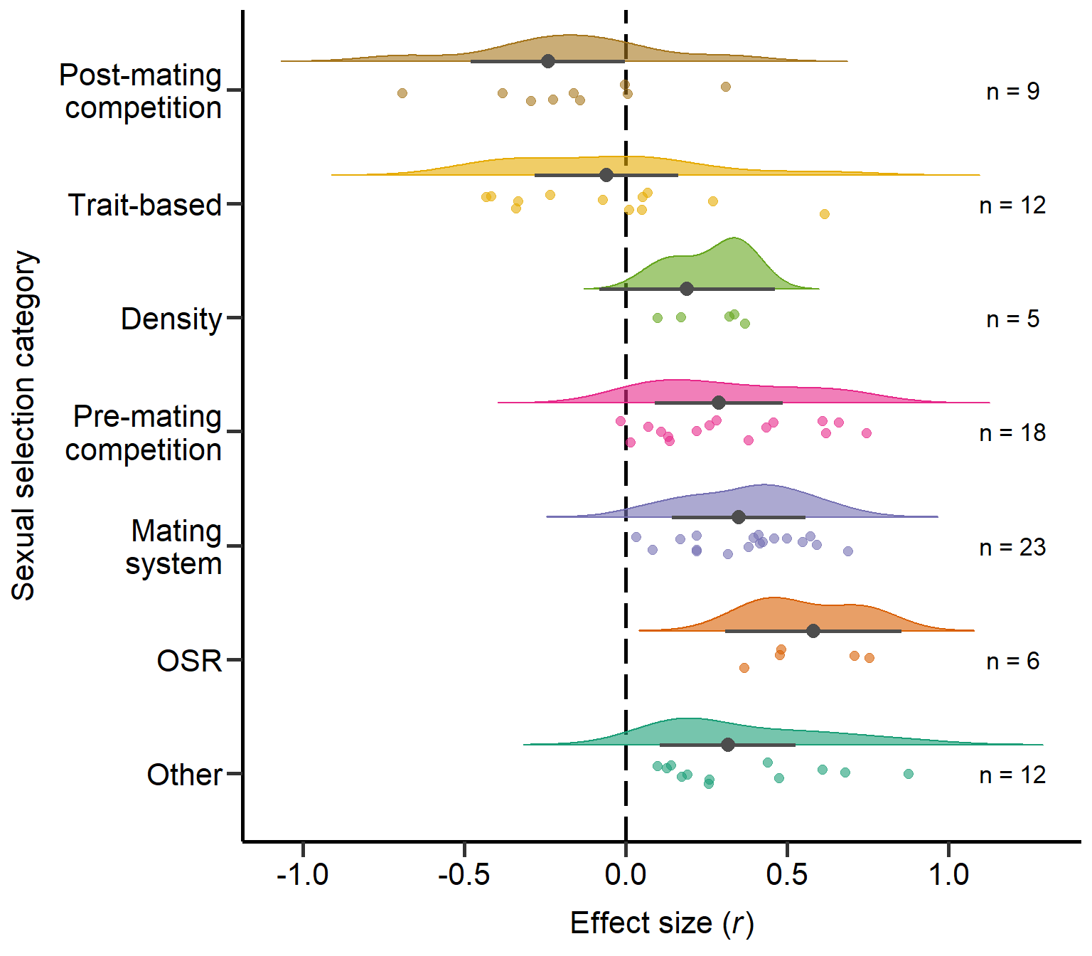

Figure S1: Raincloud plot of correlation coefficients between SSD and different sexual selection categories including sample sizes and estimates with 95%CI from phylogenetic model.

Type of SSD measure

Next we explored the effect of the type of SSD measure (i.e. body mass or size):

MetaData$SSD_Proxy=as.factor(MetaData$SSD_Proxy)
MetaData$SSD_Proxy=relevel(MetaData$SSD_Proxy,c("Body mass"))
Model_REML_by_SSDMeasure = rma.mv(r ~ SSD_Proxy, V=Var_r, data = MetaData, random = c(~ 1 | Study_ID,~ 1 | Index, ~ 1 | Class), R = list(Class = forcedC_Moderators), method = "REML")
summary(Model_REML_by_SSDMeasure)


Multivariate Meta-Analysis Model (k = 75; method: REML)

  logLik  Deviance       AIC       BIC      AICc   
-19.3875   38.7751   48.7751   60.2274   49.6706   

Variance Components:

            estim    sqrt  nlvls  fixed    factor    R 
sigma^2.1  0.0000  0.0000     44     no  Study_ID   no 
sigma^2.2  0.0799  0.2826     75     no     Index   no 
sigma^2.3  0.0120  0.1095      9     no     Class  yes 

Test for Residual Heterogeneity:
QE(df = 73) = 1137.0026, p-val < .0001

Test of Moderators (coefficient 2):
QM(df = 1) = 2.4142, p-val = 0.1202

Model Results:

                    estimate      se     zval    pval    ci.lb   ci.ub     
intrcpt               0.3354  0.1021   3.2857  0.0010   0.1353  0.5354  ** 
SSD_ProxyBody size   -0.1372  0.0883  -1.5538  0.1202  -0.3102  0.0359     

---
Signif. codes:  0 '***' 0.001 '**' 0.01 '*' 0.05 '.' 0.1 ' ' 1

We then re-leveled the model for post-hoc comparisons:

MetaData$SSD_Proxy=relevel(MetaData$SSD_Proxy,c("Body size"))
Model_REML_by_SSDMeasure2 = rma.mv(r ~ SSD_Proxy, V=Var_r, data = MetaData, random = c(~ 1 | Study_ID,~ 1 | Index, ~ 1 | Class), R = list(Class = forcedC_Moderators), method = "REML")
summary(Model_REML_by_SSDMeasure2)

Finally, we computed FDR corrected p-values:

tab3=as.data.frame(round(p.adjust(c(0.0004, 0.0008), method = 'fdr'),digit=3),row.names=cbind("Body mass","Body size"))
colnames(tab3)<-cbind('P-value')
tab3

          P-value
Body mass   0.001
Body size   0.001

Plot Type of SSD measure (Figure S2A)

Here we plot the type of SSD measure moderator:

MetaData_NAProxy=MetaData[!is.na(MetaData$SSD_Proxy),]
MetaData_NAProxy$SSD_Proxy=as.factor(MetaData_NAProxy$SSD_Proxy)
MetaData_NAProxy$SSD_Proxy=relevel(MetaData_NAProxy$SSD_Proxy,c("Body size"))

ggplot(MetaData_NAProxy, aes(x=SSD_Proxy, y=r, fill = SSD_Proxy, colour = SSD_Proxy)) +
  geom_hline(yintercept=0, linetype="longdash", color = "black", linewidth=1)+
  geom_flat_violin(position = position_nudge(x = 0.25, y = 0),adjust =1, trim = F,alpha=0.6)+
  geom_point(position = position_jitter(width = .1), size = 2.5,alpha=0.6,stroke=0,shape=19)+
  geom_point(inherit.aes = F,mapping = aes(y=Model_REML_by_SSDMeasure$b[1,1], x=2.25), size = 3.5,alpha=1,stroke=0,shape=19,color='grey30')+
  geom_point(inherit.aes = F,mapping = aes(y=Model_REML_by_SSDMeasure2$b[1,1], x=1.25), size = 3.5,alpha=1,stroke=0,shape=19,color='grey30')+
  geom_segment(inherit.aes = F,mapping = aes(y=Model_REML_by_SSDMeasure$ci.lb[1], x=2.25, xend= 2.25, yend= Model_REML_by_SSDMeasure$ci.ub[1]), alpha=1,linewidth=1,color='grey30')+
  geom_segment(inherit.aes = F,mapping = aes(y=Model_REML_by_SSDMeasure2$ci.lb[1], x=1.25, xend= 1.25, yend= Model_REML_by_SSDMeasure2$ci.ub[1]), alpha=1,linewidth=1,color='grey30')+
  ylab(expression(paste("Effect size (", italic("r"),')')))+xlab('Type of SSD measure')+coord_flip()+guides(fill = FALSE, colour = FALSE) +
  scale_color_manual(values =colpal4)+
  scale_fill_manual(values =colpal4)+
  scale_x_discrete(labels=rev(c("Body mass","Body size")),expand=c(.15,0))+
  annotate("text", x=2, y=1.2, label= "n = 37",size=4.5) +
  annotate("text", x=1, y=1.2, label= "n = 46",size=4.5)  + theme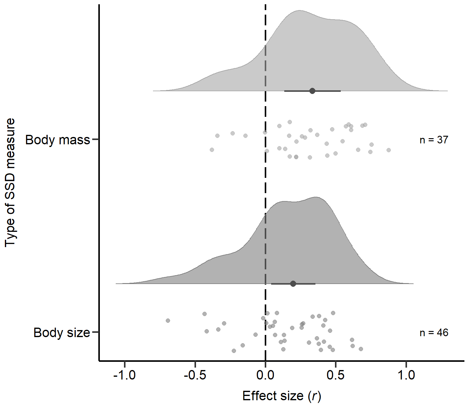

Figure S2A: Raincloud plot of correlation coefficients for different types of SSD measures (i.e. body mass or size) including sample sizes and estimates with 95% CI from phylogenetic model.

SSD measure controlled for body size?

Next we explored the effect if the primary study controlled the SSD for body size (i.e. uncontrolled or controlled):

MetaData$BodySizeControlled=as.factor(MetaData$BodySizeControlled)
MetaData$BodySizeControlled=relevel(MetaData$BodySizeControlled,c("No"))
Model_REML_by_BodySizeCont = rma.mv(r ~ BodySizeControlled, V=Var_r, data = MetaData, random = c(~ 1 | Study_ID,~ 1 | Index, ~ 1 | Class), R = list(Class = forcedC_Moderators), method = "REML")
summary(Model_REML_by_BodySizeCont)


Multivariate Meta-Analysis Model (k = 77; method: REML)

  logLik  Deviance       AIC       BIC      AICc   
-19.8069   39.6139   49.6139   61.2013   50.4835   

Variance Components:

            estim    sqrt  nlvls  fixed    factor    R 
sigma^2.1  0.0000  0.0000     45     no  Study_ID   no 
sigma^2.2  0.0768  0.2772     77     no     Index   no 
sigma^2.3  0.0236  0.1537      9     no     Class  yes 

Test for Residual Heterogeneity:
QE(df = 75) = 1181.8972, p-val < .0001

Test of Moderators (coefficient 2):
QM(df = 1) = 0.0691, p-val = 0.7927

Model Results:

                       estimate      se     zval    pval    ci.lb   ci.ub    
intrcpt                  0.2405  0.0995   2.4185  0.0156   0.0456  0.4355  * 
BodySizeControlledYes   -0.0266  0.1013  -0.2628  0.7927  -0.2252  0.1719    

---
Signif. codes:  0 '***' 0.001 '**' 0.01 '*' 0.05 '.' 0.1 ' ' 1

We then re-leveled the model for post-hoc comparisons:

MetaData$BodySizeControlled=relevel(MetaData$BodySizeControlled,c("Yes"))
Model_REML_by_BodySizeCont2 = rma.mv(r ~ BodySizeControlled, V=Var_r, data = MetaData, random = c(~ 1 | Study_ID,~ 1 | Index, ~ 1 | Class), R = list(Class = forcedC_Moderators), method = "REML")
summary(Model_REML_by_BodySizeCont2)

Finally, we computed FDR corrected p-values:

tab4=as.data.frame(round(p.adjust(c(0.0006, 0.0337), method = 'fdr'),digit=3),row.names=cbind("uncontrolled","controlled"))
colnames(tab4)<-cbind('P-value')
tab4

             P-value
uncontrolled   0.001
controlled     0.034

Plot: SSD measure controlled for body size? (Figure S2B)

Here we plot effect sizes if type of SSD measure controlled for body size:

MetaData$BodySizeControlled=as.factor(MetaData$BodySizeControlled)
MetaData$BodySizeControlled=relevel(MetaData$BodySizeControlled,c("Yes"))

ggplot(MetaData, aes(x=BodySizeControlled, y=r, fill = BodySizeControlled, colour = BodySizeControlled)) +
  geom_hline(yintercept=0, linetype="longdash", color = "black", linewidth=1)+
  geom_flat_violin(position = position_nudge(x = 0.25, y = 0),adjust =1, trim = F,alpha=0.6)+
  geom_point(position = position_jitter(width = .1), size = 2.5,alpha=0.6,stroke=0,shape=19)+
  geom_point(inherit.aes = F,mapping = aes(y=Model_REML_by_BodySizeCont$b[1,1], x=2.25), size = 3.5,alpha=1,stroke=0,shape=19,color='grey30')+
  geom_point(inherit.aes = F,mapping = aes(y=Model_REML_by_BodySizeCont2$b[1,1], x=1.25), size = 3.5,alpha=1,stroke=0,shape=19,color='grey30')+
  geom_segment(inherit.aes = F,mapping = aes(y=Model_REML_by_BodySizeCont$ci.lb[1], x=2.25, xend= 2.25, yend= Model_REML_by_BodySizeCont$ci.ub[1]), alpha=1,linewidth=1,color='grey30')+
  geom_segment(inherit.aes = F,mapping = aes(y=Model_REML_by_BodySizeCont2$ci.lb[1], x=1.25, xend= 1.25, yend= Model_REML_by_BodySizeCont2$ci.ub[1]), alpha=1,linewidth=1,color='grey30')+
  ylab(expression(paste("Effect size (", italic("r"),')')))+xlab('SSD controlled for body size?')+coord_flip()+guides(fill = FALSE, colour = FALSE) +
  scale_color_manual(values =colpal4)+
  scale_fill_manual(values =colpal4)+
  scale_x_discrete(labels=(c("Controlled","Uncontrolled")),expand=c(.15,0))+
  annotate("text", x=2, y=1.2, label= "n = 69",size=4.5) +
  annotate("text", x=1, y=1.2, label= "n = 16",size=4.5)  + theme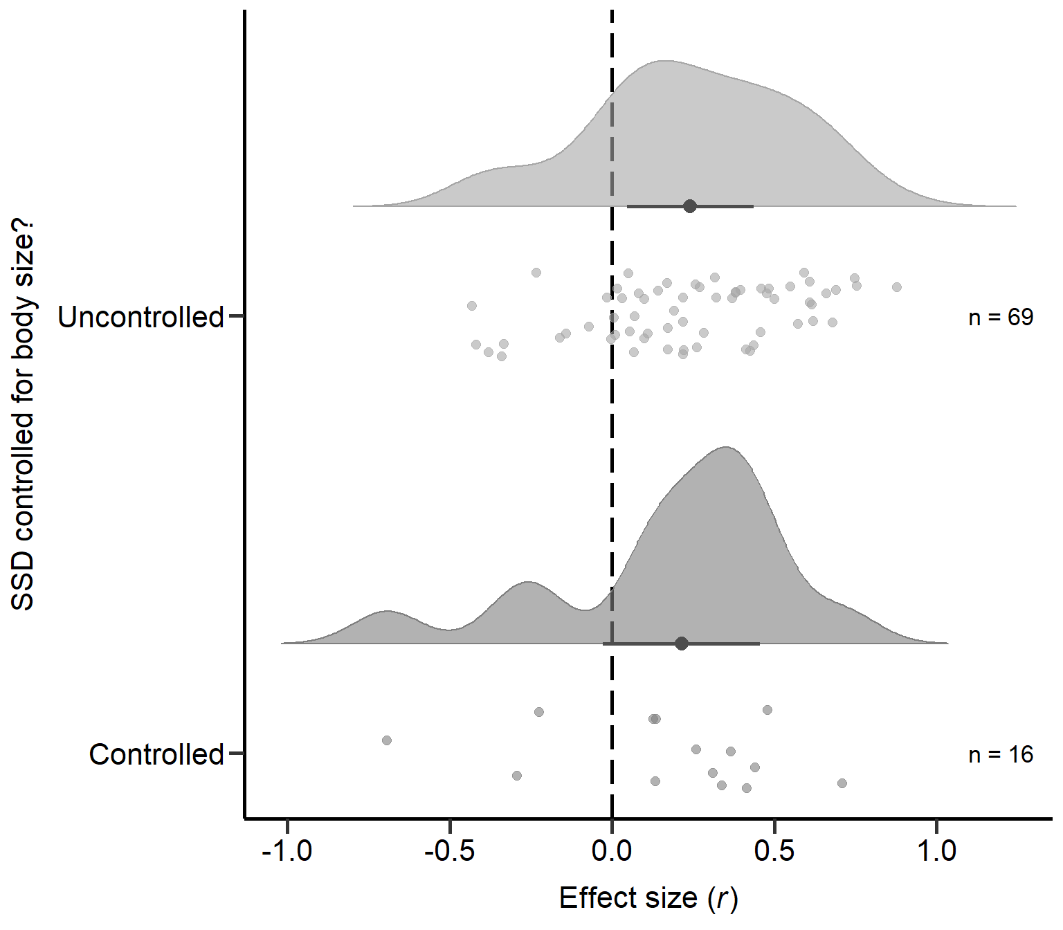

Figure S2B: Raincloud plot of correlation coefficients for primary studies controlling SSD for body size or mass (uncontrolled or controlled) including sample sizes and estimates with 95% CI from phylogenetic model.

Test for publication bias

To test for publication bias, we transformed r into z scores and ran multilevel mixed-effects models (restricted maximum likelihood) with z as the predictor and its standard error as the response with study ID and an observation level random effect. Models were weight by the mean standard error of z across all studies. While the variance in r depends on the effect size and the sample size, the variance in z is only dependent on the sample size. Hence, if z values correlate with the variance in z, this indicates that small studies were only published, if the effect was large, suggesting publication bias.

Model_REML_PublBias         = rma.mv(z ~ SE_z, V=rep((mean(SE_z)*mean(SE_z))*N,length(SE_z)), data = MetaData, random = c(~ 1 | Study_ID,~ 1 | Index, ~ 1 | Class), R = list(Class = forcedC_Moderators), method = "REML",control=list(rel.tol=1e-8))
summary(Model_REML_PublBias)


Multivariate Meta-Analysis Model (k = 77; method: REML)

  logLik  Deviance       AIC       BIC      AICc   
-91.3260  182.6520  192.6520  204.2394  193.5215   

Variance Components:

            estim    sqrt  nlvls  fixed    factor    R 
sigma^2.1  0.0000  0.0000     45     no  Study_ID   no 
sigma^2.2  0.0000  0.0000     77     no     Index   no 
sigma^2.3  0.0000  0.0003      9     no     Class  yes 

Test for Residual Heterogeneity:
QE(df = 75) = 14.1179, p-val = 1.0000

Test of Moderators (coefficient 2):
QM(df = 1) = 2.5184, p-val = 0.1125

Model Results:

         estimate      se    zval    pval    ci.lb   ci.ub    
intrcpt    0.0245  0.2601  0.0941  0.9250  -0.4853  0.5343    
SE_z       1.5405  0.9708  1.5869  0.1125  -0.3621  3.4432    

---
Signif. codes:  0 '***' 0.001 '**' 0.01 '*' 0.05 '.' 0.1 ' ' 1

Figure S2D

# Extract model predictions
model_p2 <- predict(Model_REML_PublBias)

ggplot(MetaData, aes(x=SE_z, y=z)) +
  theme(panel.grid.major = element_blank(), panel.grid.minor = element_blank(),panel.background = element_blank(), axis.line = element_line(colour = "black"))+
  theme(axis.text=element_text(size=13),
        axis.title=element_text(size=14))+ theme(legend.position="none")+ylab(expression(paste("Effect size (", italic("z"),')')))+
  geom_point(shape=16, size = 3,alpha=0.5)+xlab('Standard error')+
  geom_hline(yintercept=0, linetype="dashed", color = "black", linewidth=1)+
  geom_line( aes(y = model_p2$pred), size = 1)+ 
  geom_ribbon( aes(ymin = model_p2$ci.lb, ymax = model_p2$ci.ub, color = 'black',linetype=NA), alpha = .15,show.legend = F, outline.type = "both") +
  theme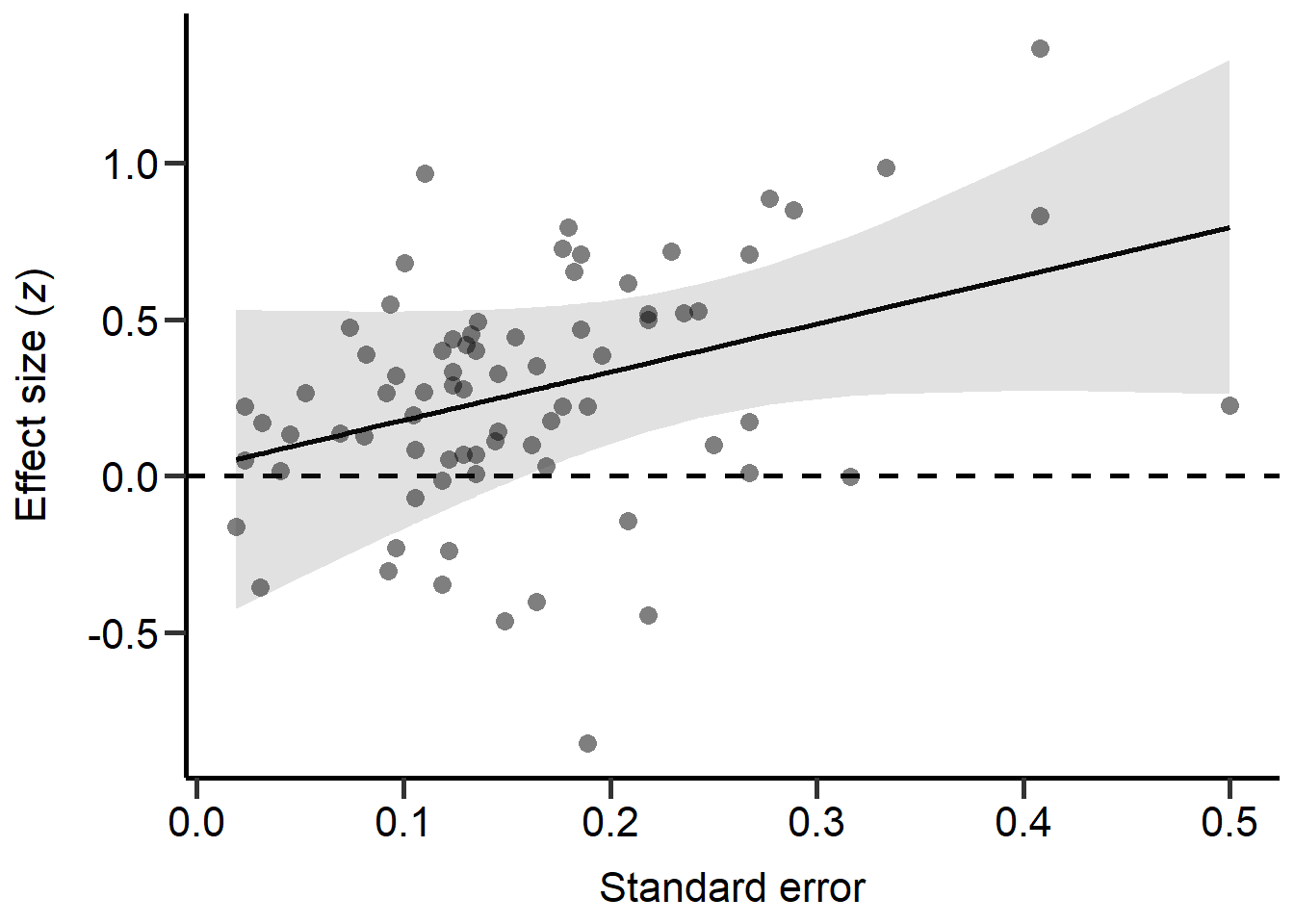

Figure S2D: Scatter plot of the standard error in z scores of each study against the z score of each primary study (transformed correlation coefficients). Dashed line marks a correlation coefficient of zero, black line represents predictions from REML model (controlling for phylogeny) and grey area represents 95% CI on model predictions.

Publication year

Next we explored the effect of the publication year of each study:

Model_REML_by_Year = rma.mv(r ~ Year, V=Var_r, data = MetaData, random = c(~ 1 | Study_ID,~ 1 | Index, ~ 1 | Class), R = list(Class = forcedC_Moderators), method = "REML",control=list(rel.tol=1e-8))
summary(Model_REML_by_Year)


Multivariate Meta-Analysis Model (k = 77; method: REML)

  logLik  Deviance       AIC       BIC      AICc   
-19.5055   39.0110   49.0110   60.5985   49.8806   

Variance Components:

            estim    sqrt  nlvls  fixed    factor    R 
sigma^2.1  0.0000  0.0001     45     no  Study_ID   no 
sigma^2.2  0.0754  0.2745     77     no     Index   no 
sigma^2.3  0.0248  0.1575      9     no     Class  yes 

Test for Residual Heterogeneity:
QE(df = 75) = 1060.4395, p-val < .0001

Test of Moderators (coefficient 2):
QM(df = 1) = 0.8325, p-val = 0.3616

Model Results:

         estimate      se     zval    pval    ci.lb    ci.ub    
intrcpt    7.7711  8.2609   0.9407  0.3469  -8.4200  23.9622    
Year      -0.0037  0.0041  -0.9124  0.3616  -0.0118   0.0043    

---
Signif. codes:  0 '***' 0.001 '**' 0.01 '*' 0.05 '.' 0.1 ' ' 1

Plot publication year (Figure S2E)

Here we plot the publication year:

# Extract model predictions
Model_REML_by_Year = rma.mv(r ~ Year, V=Var_r, data = MetaData, random = c(~ 1 | Study_ID,~ 1 | Index, ~ 1 | Class), R = list(Class = forcedC_Moderators), method = "REML",control=list(rel.tol=1e-8))
model_p4 <- predict(Model_REML_by_Year)

ggplot(MetaData, aes(x=as.numeric(Year), y=r)) +
  theme(panel.grid.major = element_blank(), panel.grid.minor = element_blank(),panel.background = element_blank(), axis.line = element_line(colour = "black"))+
  theme(axis.text=element_text(size=13),
        axis.title=element_text(size=14))+ theme(legend.position="none")+
  geom_point(shape=16, size = 3,alpha=0.5)+xlab('Publication year')+ylab(expression(paste("Effect size (", italic("r"),')')))+
  geom_hline(yintercept=0, linetype="dashed", color = "black", linewidth=1)+
  geom_line( aes(y = model_p4$pred), size = 1)+ 
  geom_ribbon( aes(ymin = model_p4$ci.lb, ymax = model_p4$ci.ub, color = 'black',linetype=NA), alpha = .15,show.legend = F, outline.type = "both") +
  theme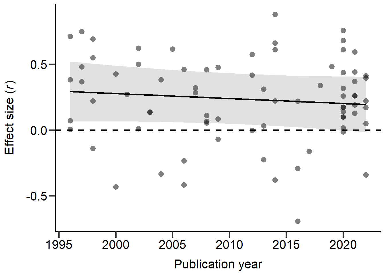

Figure S2E: Scatter plot of correlation coefficients against the publication year of each study. Dashed line marks a correlation coefficient of zero, black line represents predictions from REML model (controlling for phylogeny) and grey area represents 95% CI on model predictions.

Moderator tests for non-phylogenetic models

Here we ran all models without the phylogeny.

Sexual selection mode

The first model explores the effect of the sexual selection mode (i.e. pre-copulatory, post-copulatory or both):

MetaData$SexSel_Mode=relevel(MetaData$SexSel_Mode,c("pre-copulatory"))
Model_REML_by_cSexSelMode = rma.mv(r ~ factor(SexSel_Mode), V=Var_r, data = MetaData, random = c(~ 1 | Study_ID,~ 1 | Index), method = "REML")
summary(Model_REML_by_cSexSelMode)


Multivariate Meta-Analysis Model (k = 77; method: REML)

  logLik  Deviance       AIC       BIC      AICc   
-11.4194   22.8387   32.8387   44.3590   33.7211   

Variance Components:

            estim    sqrt  nlvls  fixed    factor 
sigma^2.1  0.0094  0.0969     45     no  Study_ID 
sigma^2.2  0.0567  0.2381     77     no     Index 

Test for Residual Heterogeneity:
QE(df = 74) = 944.4229, p-val < .0001

Test of Moderators (coefficients 2:3):
QM(df = 2) = 25.9764, p-val < .0001

Model Results:

                                    estimate      se     zval    pval    ci.lb 
intrcpt                               0.2187  0.0492   4.4484  <.0001   0.1223 
factor(SexSel_Mode)both               0.1643  0.0710   2.3126  0.0207   0.0251 
factor(SexSel_Mode)post-copulatory   -0.4065  0.1105  -3.6780  0.0002  -0.6232 
                                      ci.ub      
intrcpt                              0.3150  *** 
factor(SexSel_Mode)both              0.3036    * 
factor(SexSel_Mode)post-copulatory  -0.1899  *** 

---
Signif. codes:  0 '***' 0.001 '**' 0.01 '*' 0.05 '.' 0.1 ' ' 1

We then re-leveled the model for post-hoc comparisons:

MetaData$SexSel_Mode=relevel(MetaData$SexSel_Mode,c("post-copulatory"))
Model_REML_by_cSexSelMode2 = rma.mv(r ~ factor(SexSel_Mode), V=Var_r, data = MetaData, random = c(~ 1 | Study_ID,~ 1 | Index), method = "REML")
summary(Model_REML_by_cSexSelMode2)

MetaData$SexSel_Mode=relevel(MetaData$SexSel_Mode,c("both"))
Model_REML_by_cSexSelMode3 = rma.mv(r ~ factor(SexSel_Mode), V=Var_r, data = MetaData, random = c(~ 1 | Study_ID,~ 1 | Index),  method = "REML")
summary(Model_REML_by_cSexSelMode3)

Finally, we computed FDR corrected p-values:

tab1=as.data.frame(round(p.adjust(c(0.0001, 0.0756, .0001), method = 'fdr'),digit=3),row.names=cbind("Pre-copulatory","Post-copulatory","Both"))
colnames(tab1)<-cbind('P-value')
tab1

                P-value
Pre-copulatory    0.000
Post-copulatory   0.076
Both              0.000

Sexual selection category

Next we explored the effect of the sexual selection category (i.e. density, mating system, operational sex ratio (OSR), post-mating competition, pre-mating competition, trait-based, other):

MetaData$SexSel_Category=as.factor(MetaData$SexSel_Category)
MetaData$SexSel_Category=relevel(MetaData$SexSel_Category,c("Postmating competition"))
Model_REML_by_cSexSelCat = rma.mv(r ~ factor(SexSel_Category), V=Var_r, data = MetaData, random = c(~ 1 | Study_ID,~ 1 | Index), method = "REML")
summary(Model_REML_by_cSexSelCat)


Multivariate Meta-Analysis Model (k = 77; method: REML)

  logLik  Deviance       AIC       BIC      AICc   
 -0.3304    0.6607   18.6607   38.8972   21.6607   

Variance Components:

            estim    sqrt  nlvls  fixed    factor 
sigma^2.1  0.0196  0.1399     45     no  Study_ID 
sigma^2.2  0.0290  0.1704     77     no     Index 

Test for Residual Heterogeneity:
QE(df = 70) = 614.1683, p-val < .0001

Test of Moderators (coefficients 2:7):
QM(df = 6) = 64.8410, p-val < .0001

Model Results:

                                              estimate      se     zval    pval 
intrcpt                                        -0.1780  0.0913  -1.9498  0.0512 
factor(SexSel_Category)Other                    0.5575  0.1200   4.6453  <.0001 
factor(SexSel_Category)OSR                      0.7963  0.1520   5.2401  <.0001 
factor(SexSel_Category)Mating system            0.5724  0.1067   5.3629  <.0001 
factor(SexSel_Category)Premating competition    0.5179  0.1091   4.7481  <.0001 
factor(SexSel_Category)Density                  0.4395  0.1440   3.0525  0.0023 
factor(SexSel_Category)Trait-based              0.1278  0.1152   1.1092  0.2674 
                                                ci.lb   ci.ub      
intrcpt                                       -0.3570  0.0009    . 
factor(SexSel_Category)Other                   0.3223  0.7927  *** 
factor(SexSel_Category)OSR                     0.4985  1.0942  *** 
factor(SexSel_Category)Mating system           0.3632  0.7816  *** 
factor(SexSel_Category)Premating competition   0.3041  0.7316  *** 
factor(SexSel_Category)Density                 0.1573  0.7217   ** 
factor(SexSel_Category)Trait-based            -0.0980  0.3536      

---
Signif. codes:  0 '***' 0.001 '**' 0.01 '*' 0.05 '.' 0.1 ' ' 1

We then re-leveled the model for post-hoc comparisons:

MetaData$SexSel_Category=relevel(MetaData$SexSel_Category,c("Trait-based"))
Model_REML_by_cSexSelCat2 = rma.mv(r ~ factor(SexSel_Category), V=Var_r, data = MetaData, random = c(~ 1 | Study_ID,~ 1 | Index), method = "REML")
summary(Model_REML_by_cSexSelCat2)

MetaData$SexSel_Category=relevel(MetaData$SexSel_Category,c("Density"))
Model_REML_by_cSexSelCat3 = rma.mv(r ~ factor(SexSel_Category), V=Var_r, data = MetaData, random = c(~ 1 | Study_ID,~ 1 | Index), method = "REML")
summary(Model_REML_by_cSexSelCat3)

MetaData$SexSel_Category=relevel(MetaData$SexSel_Category,c("Premating competition"))
Model_REML_by_cSexSelCat4 = rma.mv(r ~ factor(SexSel_Category), V=Var_r, data = MetaData, random = c(~ 1 | Study_ID,~ 1 | Index), method = "REML")
summary(Model_REML_by_cSexSelCat4)

MetaData$SexSel_Category=relevel(MetaData$SexSel_Category,c("Mating system"))
Model_REML_by_cSexSelCat5 = rma.mv(r ~ factor(SexSel_Category), V=Var_r, data = MetaData, random = c(~ 1 | Study_ID,~ 1 | Index), method = "REML")
summary(Model_REML_by_cSexSelCat5)

MetaData$SexSel_Category=relevel(MetaData$SexSel_Category,c("OSR"))
Model_REML_by_cSexSelCat6 = rma.mv(r ~ factor(SexSel_Category), V=Var_r, data = MetaData, random = c(~ 1 | Study_ID,~ 1 | Index), method = "REML")
summary(Model_REML_by_cSexSelCat6)

MetaData$SexSel_Category=relevel(MetaData$SexSel_Category,c("Other"))
Model_REML_by_cSexSelCat7 = rma.mv(r ~ factor(SexSel_Category), V=Var_r, data = MetaData, random = c(~ 1 | Study_ID,~ 1 | Index), method = "REML")
summary(Model_REML_by_cSexSelCat7)

Finally, we computed FDR corrected p-values:

tab2=as.data.frame(round(p.adjust(c(0.0685, 0.5996, 0.0151, .0001, .0001, .0001, .0001), method = 'fdr'),digit=3),row.names=cbind("Postmating competition","Trait-based","Density",'Premating competition',"Mating system","OSR","Other"))
colnames(tab2)<-cbind('P-value')
tab2

                       P-value
Postmating competition   0.080
Trait-based              0.600
Density                  0.021
Premating competition    0.000
Mating system            0.000
OSR                      0.000
Other                    0.000

Phylogenetic classes

Next we explored the effect of the phylogenetic classes:

MetaData$Class=as.factor(MetaData$Class)
MetaData$Class=relevel(MetaData$Class,c("Nematoda"))
Model_cREML_by_Class = rma.mv(r ~ Class, V=Var_r, data = MetaData, random = c(~ 1 | Study_ID,~ 1 | Index), method = "REML")
summary(Model_cREML_by_Class)


Multivariate Meta-Analysis Model (k = 77; method: REML)

  logLik  Deviance       AIC       BIC      AICc   
-16.1287   32.2574   54.2574   78.6720   58.9717   

Variance Components:

            estim    sqrt  nlvls  fixed    factor 
sigma^2.1  0.0000  0.0000     45     no  Study_ID 
sigma^2.2  0.0774  0.2782     77     no     Index 

Test for Residual Heterogeneity:
QE(df = 68) = 776.5810, p-val < .0001

Test of Moderators (coefficients 2:9):
QM(df = 8) = 17.6591, p-val = 0.0239

Model Results:

                     estimate      se     zval    pval    ci.lb   ci.ub    
intrcpt                0.4222  0.2298   1.8376  0.0661  -0.0281  0.8726  . 
ClassActinopterygii   -0.2636  0.2605  -1.0118  0.3116  -0.7741  0.2470    
ClassAmphibia         -0.3092  0.2763  -1.1189  0.2632  -0.8507  0.2324    
ClassAnimalia         -0.1963  0.3107  -0.6318  0.5275  -0.8053  0.4127    
ClassAves             -0.3019  0.2390  -1.2629  0.2066  -0.7704  0.1666    
ClassInsecta          -0.1607  0.2684  -0.5987  0.5494  -0.6866  0.3653    
ClassMammalia         -0.0199  0.2370  -0.0841  0.9329  -0.4844  0.4445    
ClassPisces           -0.1639  0.3641  -0.4502  0.6526  -0.8776  0.5498    
ClassReptilia         -0.4246  0.2551  -1.6645  0.0960  -0.9246  0.0754  . 

---
Signif. codes:  0 '***' 0.001 '**' 0.01 '*' 0.05 '.' 0.1 ' ' 1

We then re-leveled the model for post-hoc comparisons:

MetaData$Class=relevel(MetaData$Class,c("Insecta"))
Model_cREML_by_Class2 = rma.mv(r ~ Class, V=Var_r, data = MetaData, random = c(~ 1 | Study_ID,~ 1 | Index), method = "REML")
summary(Model_cREML_by_Class2)

MetaData$Class=relevel(MetaData$Class,c("Aves"))
Model_cREML_by_Class3 = rma.mv(r ~ Class, V=Var_r, data = MetaData, random = c(~ 1 | Study_ID,~ 1 | Index), method = "REML")
summary(Model_cREML_by_Class3)

MetaData$Class=relevel(MetaData$Class,c("Reptilia"))
Model_cREML_by_Class4 = rma.mv(r ~ Class, V=Var_r, data = MetaData, random = c(~ 1 | Study_ID,~ 1 | Index), method = "REML")
summary(Model_cREML_by_Class4)

MetaData$Class=relevel(MetaData$Class,c("Mammalia"))
Model_cREML_by_Class5 = rma.mv(r ~ Class, V=Var_r, data = MetaData, random = c(~ 1 | Study_ID,~ 1 | Index), method = "REML")
summary(Model_cREML_by_Class5)

MetaData$Class=relevel(MetaData$Class,c("Amphibia"))
Model_cREML_by_Class6 = rma.mv(r ~ Class, V=Var_r, data = MetaData, random = c(~ 1 | Study_ID,~ 1 | Index), method = "REML")
summary(Model_cREML_by_Class6)

MetaData$Class=relevel(MetaData$Class,c("Actinopterygii"))
Model_cREML_by_Class7 = rma.mv(r ~ Class, V=Var_r, data = MetaData, random = c(~ 1 | Study_ID,~ 1 | Index), method = "REML")
summary(Model_cREML_by_Class7)


MetaData$Class=relevel(MetaData$Class,c("Pisces"))
Model_cREML_by_Class8 = rma.mv(r ~ Class, V=Var_r, data = MetaData, random = c(~ 1 | Study_ID,~ 1 | Index), method = "REML")
summary(Model_cREML_by_Class8)

MetaData$Class=relevel(MetaData$Class,c("Animalia"))
Model_cREML_by_Class9 = rma.mv(r ~ Class, V=Var_r, data = MetaData, random = c(~ 1 | Study_ID,~ 1 | Index), method = "REML")
summary(Model_cREML_by_Class9)

Finally, we computed FDR corrected p-values:

tab2=as.data.frame(round(p.adjust(c(0.2557       ,0.4534     , 0.3747    ,0.0048    ,0.0016    ,.0001  ,0.1202    , 0.3966  ,0.4405       ), method = 'fdr'),digit=3),row.names=cbind( "Nematoda","Insecta","Aves","Reptilia","Mammalia","Amphibia","Actinopterygii","Pisces","Animalia"))
colnames(tab2)<-cbind('P-value')
tab2

               P-value
Nematoda         0.453
Insecta          0.453
Aves             0.453
Reptilia         0.014
Mammalia         0.007
Amphibia         0.001
Actinopterygii   0.270
Pisces           0.453
Animalia         0.453

Plot phylogenetic classes (Figure 3)

Here we plot the phylogenetic classes:

MetaData$Class=as.factor(MetaData$Class)
MetaData$Class=factor(MetaData$Class, levels = (c("Animalia","Pisces" ,"Actinopterygii","Amphibia","Mammalia","Reptilia","Aves","Insecta","Nematoda")))

ggplot(MetaData, aes(x=Class, y=r, fill = Class, colour = Class)) +
  geom_hline(yintercept=0, linetype="longdash", color = "black", linewidth=1)+
  geom_point(position = position_jitter(width = .1), size = 2.5,alpha=0.8,stroke=0,shape=19)+
  geom_point(inherit.aes = F,mapping = aes(y=Model_cREML_by_Class$b[1,1], x=9.35), size = 3.5,alpha=1,stroke=0,shape=19,color=colpal3[9])+
  geom_point(inherit.aes = F,mapping = aes(y=Model_cREML_by_Class2$b[1,1], x=8.35), size = 3.5,alpha=1,stroke=0,shape=19,color=colpal3[8])+
  geom_point(inherit.aes = F,mapping = aes(y=Model_cREML_by_Class3$b[1,1], x=7.35), size = 3.5,alpha=1,stroke=0,shape=19,color=colpal3[7])+
  geom_point(inherit.aes = F,mapping = aes(y=Model_cREML_by_Class4$b[1,1], x=6.35), size = 3.5,alpha=1,stroke=0,shape=19,color=colpal3[6])+
  geom_point(inherit.aes = F,mapping = aes(y=Model_cREML_by_Class5$b[1,1], x=5.35), size = 3.5,alpha=1,stroke=0,shape=19,color=colpal3[5])+
  geom_point(inherit.aes = F,mapping = aes(y=Model_cREML_by_Class6$b[1,1], x=4.35), size = 3.5,alpha=1,stroke=0,shape=19,color=colpal3[4])+
  geom_point(inherit.aes = F,mapping = aes(y=Model_cREML_by_Class7$b[1,1], x=3.35), size = 3.5,alpha=1,stroke=0,shape=19,color=colpal3[3])+
  geom_point(inherit.aes = F,mapping = aes(y=Model_cREML_by_Class8$b[1,1], x=2.35), size = 3.5,alpha=1,stroke=0,shape=19,color=colpal3[2])+
  geom_point(inherit.aes = F,mapping = aes(y=Model_cREML_by_Class9$b[1,1], x=1.35), size = 3.5,alpha=1,stroke=0,shape=19,color=colpal3[1])+
  geom_segment(inherit.aes = F,mapping = aes(y=Model_cREML_by_Class$ci.lb[1], x=9.35, xend= 9.35, yend= Model_cREML_by_Class$ci.ub[1]), alpha=1,linewidth=1,color=colpal3[9])+
  geom_segment(inherit.aes = F,mapping = aes(y=Model_cREML_by_Class2$ci.lb[1], x=8.35, xend= 8.35, yend= Model_cREML_by_Class2$ci.ub[1]), alpha=1,linewidth=1,color=colpal3[8])+
  geom_segment(inherit.aes = F,mapping = aes(y=Model_cREML_by_Class3$ci.lb[1], x=7.35, xend= 7.35, yend= Model_cREML_by_Class3$ci.ub[1]), alpha=1,linewidth=1,color=colpal3[7])+
  geom_segment(inherit.aes = F,mapping = aes(y=Model_cREML_by_Class4$ci.lb[1], x=6.35, xend= 6.35, yend= Model_cREML_by_Class4$ci.ub[1]), alpha=1,linewidth=1,color=colpal3[6])+
  geom_segment(inherit.aes = F,mapping = aes(y=Model_cREML_by_Class5$ci.lb[1], x=5.35, xend= 5.35, yend= Model_cREML_by_Class5$ci.ub[1]), alpha=1,linewidth=1,color=colpal3[5])+
  geom_segment(inherit.aes = F,mapping = aes(y=Model_cREML_by_Class6$ci.lb[1], x=4.35, xend= 4.35, yend= Model_cREML_by_Class6$ci.ub[1]), alpha=1,linewidth=1,color=colpal3[4])+
  geom_segment(inherit.aes = F,mapping = aes(y=Model_cREML_by_Class7$ci.lb[1], x=3.35, xend= 3.35, yend= Model_cREML_by_Class7$ci.ub[1]), alpha=1,linewidth=1,color=colpal3[3])+
  geom_segment(inherit.aes = F,mapping = aes(y=Model_cREML_by_Class8$ci.lb[1], x=2.35, xend= 2.35, yend= Model_cREML_by_Class8$ci.ub[1]), alpha=1,linewidth=1,color=colpal3[2])+
  geom_segment(inherit.aes = F,mapping = aes(y=Model_cREML_by_Class9$ci.lb[1], x=1.35, xend= 1.35, yend= Model_cREML_by_Class9$ci.ub[1]), alpha=1,linewidth=1,color=colpal3[1])+
  ylab(expression(paste("Effect size (", italic("r"),')')))+xlab('Class')+coord_flip()+guides(fill = FALSE, colour = FALSE) +
  scale_color_manual(values =colpal3)+
  scale_fill_manual(values =colpal3)+
  scale_x_discrete(labels=(c("Animalia","Pisces" ,"Actinopterygii","Amphibia","Mammalia","Reptilia","Aves","Insecta","Nematoda")),expand=c(.1,0))+
  theme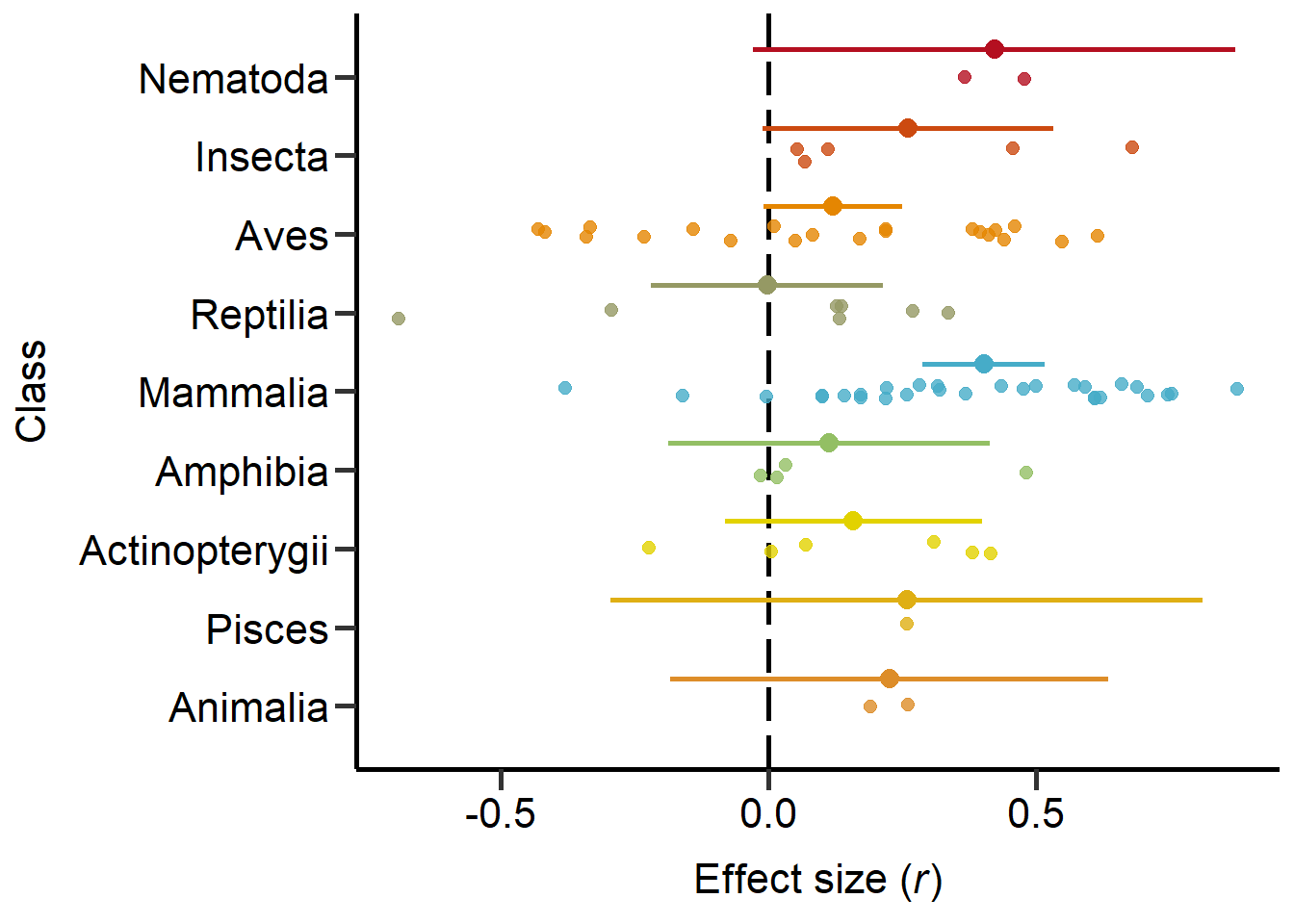

Figure 3: Phylogeny based on classes including sample sizes for the number of studies and number of effect sizes, respectively, and estimates with 95%CI from non-phylogenetic model.

Type of SSD measure

Next we explored the effect of the type of SSD measure (i.e. body mass or size):

MetaData$SSD_Proxy=as.factor(MetaData$SSD_Proxy)
MetaData$SSD_Proxy=relevel(MetaData$SSD_Proxy,c("Body mass"))
Model_REML_by_cSSDMeasure = rma.mv(r ~ SSD_Proxy, V=Var_r, data = MetaData, random = c(~ 1 | Study_ID,~ 1 | Index), method = "REML")
summary(Model_REML_by_cSSDMeasure)


Multivariate Meta-Analysis Model (k = 75; method: REML)

  logLik  Deviance       AIC       BIC      AICc   
-20.0151   40.0302   48.0302   57.1920   48.6184   

Variance Components:

            estim    sqrt  nlvls  fixed    factor 
sigma^2.1  0.0000  0.0000     44     no  Study_ID 
sigma^2.2  0.0856  0.2925     75     no     Index 

Test for Residual Heterogeneity:
QE(df = 73) = 1137.0026, p-val < .0001

Test of Moderators (coefficient 2):
QM(df = 1) = 6.0488, p-val = 0.0139

Model Results:

                    estimate      se     zval    pval    ci.lb    ci.ub      
intrcpt               0.3367  0.0549   6.1291  <.0001   0.2290   0.4443  *** 
SSD_ProxyBody size   -0.1825  0.0742  -2.4594  0.0139  -0.3279  -0.0371    * 

---
Signif. codes:  0 '***' 0.001 '**' 0.01 '*' 0.05 '.' 0.1 ' ' 1

We then re-leveled the model for post-hoc comparisons:

MetaData$SSD_Proxy=relevel(MetaData$SSD_Proxy,c("Body size"))
Model_REML_by_cSSDMeasure2 = rma.mv(r ~ SSD_Proxy, V=Var_r, data = MetaData, random = c(~ 1 | Study_ID,~ 1 | Index), method = "REML")
summary(Model_REML_by_cSSDMeasure2)

Finally, we computed FDR corrected p-values:

tab3=as.data.frame(round(p.adjust(c(.0001, .0001), method = 'fdr'),digit=3),row.names=cbind("Body mass","Body size"))
colnames(tab3)<-cbind('P-value')
tab3

          P-value
Body mass       0
Body size       0

SSD measure controlled for body size?

Next we explored the effect if the primary study controlled the SSD for body size (i.e. uncontrolled or controlled):

MetaData$BodySizeControlled=as.factor(MetaData$BodySizeControlled)
MetaData$BodySizeControlled=relevel(MetaData$BodySizeControlled,c("No"))
Model_REML_by_cBodySizeCont = rma.mv(r ~ BodySizeControlled, V=Var_r, data = MetaData, random = c(~ 1 | Study_ID,~ 1 | Index), method = "REML")
summary(Model_REML_by_cBodySizeCont)


Multivariate Meta-Analysis Model (k = 77; method: REML)

  logLik  Deviance       AIC       BIC      AICc   
-22.0756   44.1512   52.1512   61.4212   52.7227   

Variance Components:

            estim    sqrt  nlvls  fixed    factor 
sigma^2.1  0.0149  0.1220     45     no  Study_ID 
sigma^2.2  0.0769  0.2773     77     no     Index 

Test for Residual Heterogeneity:
QE(df = 75) = 1181.8972, p-val < .0001

Test of Moderators (coefficient 2):
QM(df = 1) = 0.5960, p-val = 0.4401

Model Results:

                       estimate      se     zval    pval    ci.lb   ci.ub      
intrcpt                  0.2547  0.0447   5.6926  <.0001   0.1670  0.3424  *** 
BodySizeControlledYes   -0.0787  0.1020  -0.7720  0.4401  -0.2786  0.1212      

---
Signif. codes:  0 '***' 0.001 '**' 0.01 '*' 0.05 '.' 0.1 ' ' 1

We then re-leveled the model for post-hoc comparisons:

MetaData$BodySizeControlled=relevel(MetaData$BodySizeControlled,c("Yes"))
Model_REML_by_cBodySizeCont2 = rma.mv(r ~ BodySizeControlled, V=Var_r, data = MetaData, random = c(~ 1 | Study_ID,~ 1 | Index), method = "REML")
summary(Model_REML_by_cBodySizeCont2)

Finally, we computed FDR corrected p-values:

tab4=as.data.frame(round(p.adjust(c(.0001, 0.0168), method = 'fdr'),digit=3),row.names=cbind("uncontrolled","controlled"))
colnames(tab4)<-cbind('P-value')
tab4

             P-value
uncontrolled   0.000
controlled     0.017

Test for publication bias

Model_cREML_PublBias         = rma.mv(z ~ SE_z, V=rep(((mean(SE_z)*mean(SE_z))*N),length(SE_z)), data = MetaData, random = c(~ 1 | Study_ID,~ 1 | Index), method = "REML")
summary(Model_cREML_PublBias)


Multivariate Meta-Analysis Model (k = 77; method: REML)

  logLik  Deviance       AIC       BIC      AICc   
-91.3260  182.6520  190.6520  199.9219  191.2234   

Variance Components:

            estim    sqrt  nlvls  fixed    factor 
sigma^2.1  0.0000  0.0000     45     no  Study_ID 
sigma^2.2  0.0000  0.0000     77     no     Index 

Test for Residual Heterogeneity:
QE(df = 75) = 14.1179, p-val = 1.0000

Test of Moderators (coefficient 2):
QM(df = 1) = 2.5184, p-val = 0.1125

Model Results:

         estimate      se    zval    pval    ci.lb   ci.ub    
intrcpt    0.0245  0.2601  0.0941  0.9250  -0.4853  0.5343    
SE_z       1.5405  0.9708  1.5869  0.1125  -0.3621  3.4432    

---
Signif. codes:  0 '***' 0.001 '**' 0.01 '*' 0.05 '.' 0.1 ' ' 1

Publication year

Next we explored the effect of the publication year of each study:

Model_cREML_by_Year = rma.mv(r ~ Year, V=Var_r, data = MetaData, random = c(~ 1 | Study_ID,~ 1 | Index), method = "REML")
summary(Model_cREML_by_Year)


Multivariate Meta-Analysis Model (k = 77; method: REML)

  logLik  Deviance       AIC       BIC      AICc   
-22.0838   44.1677   52.1677   61.4376   52.7391   

Variance Components:

            estim    sqrt  nlvls  fixed    factor 
sigma^2.1  0.0193  0.1390     45     no  Study_ID 
sigma^2.2  0.0733  0.2707     77     no     Index 

Test for Residual Heterogeneity:
QE(df = 75) = 1060.4395, p-val < .0001

Test of Moderators (coefficient 2):
QM(df = 1) = 0.5199, p-val = 0.4709

Model Results:

         estimate      se     zval    pval     ci.lb    ci.ub    
intrcpt    7.0575  9.4535   0.7466  0.4553  -11.4710  25.5860    
Year      -0.0034  0.0047  -0.7210  0.4709   -0.0126   0.0058    

---
Signif. codes:  0 '***' 0.001 '**' 0.01 '*' 0.05 '.' 0.1 ' ' 1

Forest plot

# Sort data by Class
MetaData$Class=as.factor(MetaData$Class)
MetaData$Class=factor(MetaData$Class, levels = c("Animalia","Pisces" ,"Actinopterygii","Amphibia","Mammalia","Reptilia","Aves","Insecta","Nematoda"))
MetaData_sorted <-MetaData[order(MetaData$Class),]

# Add global effect size to data
forestData=MetaData_sorted[,c(3,5,12,17,20,21)]
GlobalES=as.data.frame(cbind('Global effect size','','Global effect size',Model_REML_Null$b[1,1],Model_REML_Null$ci.lb[1],Model_REML_Null$ci.ub[1]))
colnames(GlobalES)=c('AuthorsAndYear','Class','SexSel_Mode','r','lCI','uCI')
forestData=rbind(GlobalES,forestData)
forestData[,c(4:6)]=lapply(forestData[,c(4:6)],as.numeric)
forestData$SexSel_Mode=as.factor(forestData$SexSel_Mode)
forestData$SexSel_Mode=factor(forestData$SexSel_Mode, levels = c("pre-copulatory","post-copulatory" ,"both","Global effect size"))

Figure 1

ggplot(data=forestData, aes(y=1:nrow(forestData), x=r, xmin=lCI, xmax=uCI,color=SexSel_Mode)) +
  geom_vline(xintercept=0, color='black', linetype='dashed', alpha=.5,linewidth=0.8) +
  geom_point(size = ifelse(1:nrow(forestData) == c(1), 2.75, 1.8))+
  geom_errorbarh(height=0,size = ifelse(1:nrow(forestData) == c(1), 1.25, 1))+
  scale_y_continuous(breaks=seq(1, nrow(forestData), by=1), labels=forestData$AuthorsAndYear,limits=c(1,length(forestData$AuthorsAndYear)),expand=c(0.015,0.015)) +
  labs(title='', x=expression(paste(italic("r "),'(95% CI)')), y = 'Study') +
  theme_classic()+theme(axis.text.x=element_text(size=12),
                        axis.title=element_text(size=12))+ labs(color =  c("Sexual selection mode"))+ 
  scale_colour_manual(values=Meta_col, labels=c('Pre-copulatory','Post-copulatory',"Both","Global effect size"))+
  guides(color = guide_legend(override.aes = list(size = .9)))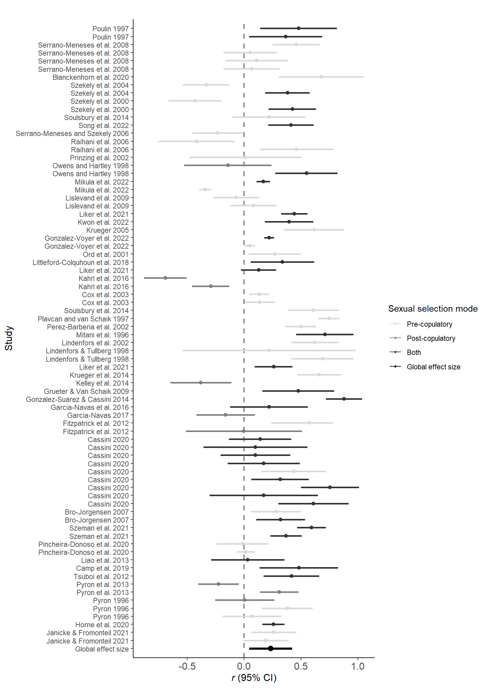

Figure 1: Forest plot including correlation coefficients (±95% CI), as well as the global effect size (in grey) with and without controlling for phylogeny. Different animal classes highlighted by background colors (see Figure 3 for class names) and sexual selection modes pre- (red), post-copulatory (blue) and both (green) by color of effect size.

sessionInfo()

R version 4.2.3 (2023-03-15 ucrt)
Platform: x86_64-w64-mingw32/x64 (64-bit)
Running under: Windows 10 x64 (build 19045)

Matrix products: default

locale:
[1] LC_COLLATE=German_Germany.utf8  LC_CTYPE=German_Germany.utf8   
[3] LC_MONETARY=German_Germany.utf8 LC_NUMERIC=C                   
[5] LC_TIME=German_Germany.utf8    

attached base packages:
[1] stats     graphics  grDevices utils     datasets  methods   base     

other attached packages:
 [1] wesanderson_0.3.6   PupillometryR_0.0.4 rlang_1.1.0        
 [4] dplyr_1.1.1         cowplot_1.1.1       ggdist_3.3.0       
 [7] MCMCglmm_2.34       coda_0.19-4         RColorBrewer_1.1-3 
[10] ggplot2_3.4.2       data.table_1.14.8   multcomp_1.4-23    
[13] TH.data_1.1-2       survival_3.5-3      mvtnorm_1.1-3      
[16] psych_2.3.3         pwr_1.3-0           MASS_7.3-58.2      
[19] metafor_4.2-0       numDeriv_2016.8-1.1 metadat_1.2-0      
[22] Matrix_1.5-3        matrixcalc_1.0-6    ape_5.7-1          
[25] workflowr_1.7.0    

loaded via a namespace (and not attached):
 [1] httr_1.4.5           sass_0.4.5           jsonlite_1.8.4      
 [4] splines_4.2.3        bslib_0.4.2          getPass_0.2-2       
 [7] distributional_0.3.2 highr_0.10           tensorA_0.36.2      
[10] yaml_2.3.7           pillar_1.9.0         lattice_0.20-45     
[13] glue_1.6.2           digest_0.6.31        promises_1.2.0.1    
[16] colorspace_2.1-0     sandwich_3.0-2       htmltools_0.5.5     
[19] httpuv_1.6.9         pkgconfig_2.0.3      corpcor_1.6.10      
[22] scales_1.2.1         processx_3.8.0       whisker_0.4.1       
[25] later_1.3.0          cubature_2.0.4.6     git2r_0.31.0        
[28] tibble_3.2.1         generics_0.1.3       farver_2.1.1        
[31] cachem_1.0.7         withr_2.5.0          cli_3.6.1           
[34] mnormt_2.1.1         magrittr_2.0.3       evaluate_0.20       
[37] ps_1.7.3             fs_1.6.1             fansi_1.0.4         
[40] nlme_3.1-162         tools_4.2.3          lifecycle_1.0.3     
[43] stringr_1.5.0        munsell_0.5.0        callr_3.7.3         
[46] compiler_4.2.3       jquerylib_0.1.4      grid_4.2.3          
[49] rstudioapi_0.14      labeling_0.4.2       rmarkdown_2.21      
[52] gtable_0.3.3         codetools_0.2-19     R6_2.5.1            
[55] zoo_1.8-12           knitr_1.42           fastmap_1.1.1       
[58] utf8_1.2.3           mathjaxr_1.6-0       rprojroot_2.0.3     
[61] stringi_1.7.12       parallel_4.2.3       Rcpp_1.0.10         
[64] vctrs_0.6.1          tidyselect_1.2.0     xfun_0.38