Transcriptome sequencing data pre-processing
Maeva Techer
2024-11-01
Last updated: 2024-11-01
Checks: 7 0
Knit directory:
locust-comparative-genomics/
This reproducible R Markdown analysis was created with workflowr (version 1.7.1). The Checks tab describes the reproducibility checks that were applied when the results were created. The Past versions tab lists the development history.
Great! Since the R Markdown file has been committed to the Git repository, you know the exact version of the code that produced these results.
Great job! The global environment was empty. Objects defined in the global environment can affect the analysis in your R Markdown file in unknown ways. For reproduciblity it’s best to always run the code in an empty environment.
The command set.seed(20221025) was run prior to running
the code in the R Markdown file. Setting a seed ensures that any results
that rely on randomness, e.g. subsampling or permutations, are
reproducible.
Great job! Recording the operating system, R version, and package versions is critical for reproducibility.
Nice! There were no cached chunks for this analysis, so you can be confident that you successfully produced the results during this run.
Great job! Using relative paths to the files within your workflowr project makes it easier to run your code on other machines.
Great! You are using Git for version control. Tracking code development and connecting the code version to the results is critical for reproducibility.
The results in this page were generated with repository version 1aaa476. See the Past versions tab to see a history of the changes made to the R Markdown and HTML files.
Note that you need to be careful to ensure that all relevant files for
the analysis have been committed to Git prior to generating the results
(you can use wflow_publish or
wflow_git_commit). workflowr only checks the R Markdown
file, but you know if there are other scripts or data files that it
depends on. Below is the status of the Git repository when the results
were generated:
Ignored files:
    Ignored:    .DS_Store
    Ignored:    .RData
    Ignored:    .Rhistory
    Ignored:    .Rproj.user/
    Ignored:    analysis/.DS_Store
    Ignored:    analysis/.Rhistory
    Ignored:    data/.DS_Store
    Ignored:    data/.Rhistory
    Ignored:    data/OLD/.DS_Store
    Ignored:    data/OLD/DEseq2_SCUBE_SCUBE_THORAX_STARnew_features/.DS_Store
    Ignored:    data/OLD/DEseq2_SGREG_SGREG_HEAD_STARnew_features/.DS_Store
    Ignored:    data/OLD/DEseq2_SGREG_SGREG_THORAX_STARnew_features/.DS_Store
    Ignored:    data/OLD/americana/.DS_Store
    Ignored:    data/OLD/americana/deg_counts/.DS_Store
    Ignored:    data/OLD/americana/deg_counts/STAR_newparams/.DS_Store
    Ignored:    data/OLD/cubense/deg_counts/STAR/cubense/featurecounts/
    Ignored:    data/OLD/cubense/deg_counts/STAR/gregaria/
    Ignored:    data/OLD/gregaria/.DS_Store
    Ignored:    data/OLD/gregaria/deg_counts/.DS_Store
    Ignored:    data/OLD/gregaria/deg_counts/STAR/.DS_Store
    Ignored:    data/OLD/gregaria/deg_counts/STAR/gregaria/.DS_Store
    Ignored:    data/OLD/gregaria/deg_counts/STAR_newparams/.DS_Store
    Ignored:    data/OLD/piceifrons/.DS_Store
    Ignored:    data/annotation/
    Ignored:    data/list/.DS_Store
    Ignored:    figures/
    Ignored:    tables/
Note that any generated files, e.g. HTML, png, CSS, etc., are not included in this status report because it is ok for generated content to have uncommitted changes.
These are the previous versions of the repository in which changes were
made to the R Markdown (analysis/3_seq-data-qc.Rmd) and
HTML (docs/3_seq-data-qc.html) files. If you’ve configured
a remote Git repository (see ?wflow_git_remote), click on
the hyperlinks in the table below to view the files as they were in that
past version.
| File | Version | Author | Date | Message |
|---|---|---|---|---|
| Rmd | f01f1cf | Maeva TECHER | 2024-11-01 | Adding new files and docs |
| html | f01f1cf | Maeva TECHER | 2024-11-01 | Adding new files and docs |
| html | ba35b82 | Maeva A. TECHER | 2024-06-20 | Build site. |
| html | b9f148d | Maeva A. TECHER | 2024-05-15 | Build site. |
| Rmd | bba0fce | Maeva A. TECHER | 2024-05-15 | wflow_publish("analysis/3_seq-data-qc.Rmd") |
| html | 178254e | Maeva A. TECHER | 2024-05-14 | Build site. |
| Rmd | be09a11 | Maeva A. TECHER | 2024-05-14 | update markdown |
| html | be09a11 | Maeva A. TECHER | 2024-05-14 | update markdown |
| html | d1cebea | Maeva A. TECHER | 2024-02-20 | Build site. |
| Rmd | 55f9385 | Maeva A. TECHER | 2024-02-20 | wflow_publish("analysis/3_seq-data-qc.Rmd") |
| html | df94db2 | Maeva A. TECHER | 2024-02-20 | adding markdown qc |
| Rmd | f6b4961 | Maeva A. TECHER | 2024-02-20 | wflow_publish("analysis/3_seq-data-qc.Rmd") |
| html | e39d280 | Maeva A. TECHER | 2024-01-30 | Build site. |
| html | f701a01 | Maeva A. TECHER | 2024-01-30 | reupdate |
| html | be046c6 | Maeva A. TECHER | 2024-01-24 | Build site. |
| html | 1b09cbe | Maeva A. TECHER | 2024-01-24 | remove |
| html | 141b63c | Maeva A. TECHER | 2023-12-18 | Build site. |
| Rmd | 53877fa | Maeva A. TECHER | 2023-12-18 | add pages |
At this point, we will have organized both SRA and de novo
paired-end sequencing data within our working
directory (for us: located on Grace cluster at
/scratch/group/songlab/maeva/headthor-locusts-rna/data) and
will be ready to run the Snakemake pipeline on it. As a reminder, each
library was build from total RNA extracted and ribodepleted (mRNA,
lncRNA, circRNA) from bulk tissues (either head or thorax) from a single
specimen reared under isolated or crowded conditions.
Load R libraries (install first from CRAN or Bioconductor)
library("knitr")
library("rmdformats")
library("tidyverse")
library("DT")  # for making interactive search table
library("plotly") # for interactive plots
library("ggthemes") # for theme_calc
library("reshape2")
library("readr")
library("ggplot2")

## Global options
options(max.print="10000")
knitr::opts_chunk$set(
    echo = TRUE,
    message = FALSE,
    warning = FALSE,
    cache = FALSE,
    comment = FALSE,
    prompt = FALSE,
    tidy = TRUE
)
opts_knit$set(width=75)
Control the quality of the .fastq files
The first step is to ensure that we have enough reads per library and
remove any potential outlier resulting from library preparation or
sequencing failure. For that, we will assess each .fastq file with
FASTQC. However, considering we are working with a
significant sample size, we will compile the results using
MULTIQC.
The aggregated results can be conveniently viewed by opening the HTML report in a web browser.
# On Grace cluster at Texas A&M University

module load GCC/12.2.0  OpenMPI/4.1.4 MultiQC/1.14
multiqc --title 'TYPE THE TITLE YOU WANT' -v /PATHTODIRECTORY
montana <- read_table("data/metadata/Stats_RNAseq_QC_19Feb2024.txt", col_names = TRUE, guess_max = 1000)
head(montana)FALSE # A tibble: 6 × 7
FALSE Sample_Name Species Perc_Dups Perc_GC M_Seqs Unique_Reads Duplicate_Reads
FALSE <chr> <chr> <dbl> <dbl> <dbl> <dbl> <dbl>
FALSE 1 SAMER_G_Crd_SRR… americ… 0.71 0.46 23.7 6958831 16765516
FALSE 2 SAMER_G_Crd_SRR… americ… 0.67 0.47 23.7 7784916 15939431
FALSE 3 SAMER_G_Crd_SRR… americ… 0.71 0.48 15.7 4570667 11085054
FALSE 4 SAMER_G_Crd_SRR… americ… 0.67 0.48 15.7 5145265 10510456
FALSE 5 SAMER_G_Crd_SRR… americ… 0.84 0.49 37.2 6049864 31125514
FALSE 6 SAMER_G_Crd_SRR… americ… 0.8 0.49 37.2 7301268 29874110# Convert values to millions
montana <- montana %>%
mutate_at(vars(contains("Reads")), list(~ ./1000000))
# Pivot the data
montana_long <- montana %>%
pivot_longer(cols = contains("Reads"), names_to = "Variable", values_to = "Value")
# Define colors
colors.reads <- c("Duplicate_Reads" = "black", "Unique_Reads" = "deepskyblue")
# Plot the stacked bar plot with values in millions and custom colors
ggplot(montana_long, aes(x = Sample_Name, y = Value, fill = Variable)) +
geom_bar(stat = "identity", position = "stack") +
facet_wrap(~Species, scales = "free") +
labs(title = "Stacked Bar Plot of Unique Reads and Duplicate Reads by Sample",
x = NULL, # Remove x-axis label
y = "Millions of Reads") +
theme_minimal() +
theme(axis.text.x = element_blank()) + # Remove x-axis labels
scale_fill_manual(values = colors.reads) + # Set custom colors
geom_hline(yintercept = 30, linetype = "dashed", color = "red") +
geom_hline(yintercept = 50, linetype = "dashed", color = "gray70") +
ylim(0, 62) # Set y-axis limits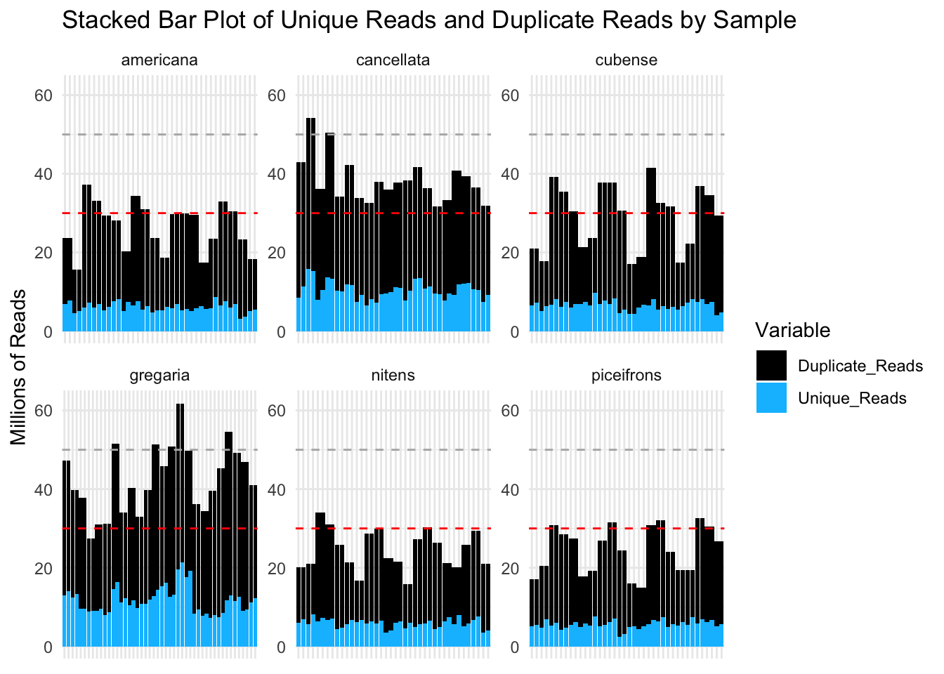
These plots show that most of our samples have over 30 million reads per sample and that most of these reads are considered duplicates. However, it is possible that the “duplicate” status come from the over expression of certain genes in Schistocerca.
library(ggConvexHull)
# Define custom colors for each species
species_colors <- c("americana" = "forestgreen", "cubense" = "yellow3", "gregaria" = "orange", "nitens" = "blue", "piceifrons" = "red2", cancellata = "deeppink")

p <- ggplot(montana, aes(x = Perc_Dups, y = M_Seqs, color = Species)) +
  geom_point(size =2) +
  scale_color_manual(values = species_colors) +  # Apply custom colors
  labs(title = "M_Seqs vs % Dups by Species",
       x = "Percentage of Duplicates",
       y = "Millions of Reads") +
  theme_minimal()

p + geom_convexhull(aes(fill = Species, color = Species), alpha = 0.2) +
    scale_fill_manual(values = species_colors)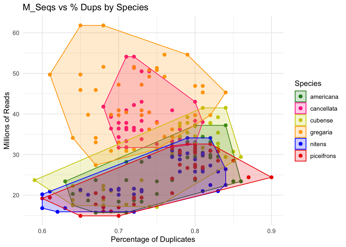
Trim and adapter removal
After checking the initial sequence quality, we can determine whether
any parameters adjustments are needed. There are several tools for
trimming and removing adapters but we used fastp and
trim_galore to remove our contaminants. Below are the two
Snakemake rules we are using. We decided to go ahead with
trim_galore as it was able to remove adapter-dimers the
best in our dataset.
########################################
# Snakefile rule
########################################

rule trimming_fastp:
        input:
                read1 = WORKDir + "/00-{species}-reads/{locust}_1.fastq.gz",
                read2 = WORKDir + "/00-{species}-reads/{locust}_2.fastq.gz"
        output:
                reportjson = WORKDir + "/01-{species}-trimmed-fastp/TrimQC/{locust}_fastp.json",
                reporthtml = WORKDir + "/01-{species}-trimmed-fastp/TrimQC/{locust}_fastp.html",
                tread1 = WORKDir + "/01-{species}-trimmed-fastp/{locust}_1.trimmed.fastq.gz",
                tread2 = WORKDir + "/01-{species}-trimmed-fastp/{locust}_2.trimmed.fastq.gz"
        shell:
                """
                module purge
                ml GCC/11.2.0 fastp/0.23.2

                fastp --thread 16 \\
                --in1 {input.read1} \\
                --in2 {input.read2} \\
                --out1 {output.tread1} \\
                --out2 {output.tread2} \\
                --trim_front1 2 \\
                --trim_front2 2 \\
                --detect_adapter_for_pe \\
                -l 50 \\
                --json {output.reportjson} \\
                --html {output.reporthtml}
                """


rule trimming_tgalore:
        input:
                read1 = WORKDir + "/00-{species}-reads/{locust}_1.fastq.gz",
                read2 = WORKDir + "/00-{species}-reads/{locust}_2.fastq.gz"
        output:
                tread1 = WORKDir + "/01-{species}-trimmed-tgalore/{locust}_1_val_1.fq.gz",
                tread2 = WORKDir + "/01-{species}-trimmed-tgalore/{locust}_2_val_2.fq.gz"
        shell:
                """
                module purge
                ml GCCcore/11.2.0 Trim_Galore/0.6.7

                trim_galore --trim-n \\
                --cores 16 \\
                --quality 20 \\
                --clip_R1 2 \\
                --clip_R2 2 \\
                --nextera \\
                --output_dir {WORKDir}/01-{wildcards.species}-trimmed-tgalore/ \\
                --fastqc \\
                --paired {input.read1} {input.read2}
                """

########################################
# Parameters in the cluster.json file
########################################

    "trimming_fastp": {
        "cpus-per-task" : 16,
        "partition" : "medium",
        "ntasks": 1,
        "mem" : "40G",
        "time": "0-12:00:00"
    },
    "trimming_tgalore": {
        "cpus-per-task" : 16,
        "partition" : "medium",
        "ntasks": 1,
        "mem" : "40G",
        "time": "0-12:00:00"
    },
For trimming with fastp, we use the following
parameters:
--in1 {input.read1}and--in2 {input.read2}: Specifies the input files in FASTQ format.--out1 {output.tread1}and--out2 {output.tread2}: Defines the output files for the trimmed reads.--trim_front1 2and--trim_front2 2: Trims the first two nucleotides from the start (5’ end) of each read in both files.--detect_adapter_for_pe: Enables automatic adapter detection for paired-end sequencing reads. This setting ensures that adapter sequences, if present, are detected and trimmed from the reads.-l 50: Sets the minimum length for reads after trimming. Any read shorter than 50 nucleotides after trimming is discarded.--json {output.reportjson}and--html {output.reporthtml}: Specifies a JSON/HTML format report file to summarize trimming statistics and quality control metrics.
For trimming with trim_galore, we use the following
parameters:
--paired {input.read1} {input.read2}: Specifies that the input is paired-end data.--output_dir {WORKDir}/01-{wildcards.species}-trimmed-tgalore/: Specifies the output directory where trimmed files will be saved.{wildcards.species}is a placeholder for the species name, allowing for organized output by species.--clip_R1 2and--clip_R2 2: Clips the first two bases from the 5’ end of both reads (R1 and R2) in paired-end sequencing.--nextera: Specifies the use of Nextera adapter sequences for trimming, which are specific to Nextera library preparations. We use this option because with FastQC we saw contaminants of these adapters in some libraries.--quality 20: Trims low-quality bases from the end of each read, keeping bases with a Phred score of 20 or higher.--fastqc: Runs FastQC after trimming to generate quality reports, allowing you to assess the quality of the trimmed reads.
Trim quality control
If you run the two rules above, you do not need to run the following Snakemake portion, but I put it in case we need to perform extra and customized quality control checks after trimming to ensure that the clipping and filtering of sequences were not overly aggressive. Given the number of sequences we work with, manually inspecting each file immediately would be time-consuming. Instead, we adopt a random sampling approach across different species, rearing conditions, and tissues to see that the trimming process worked well.
########################################
# Snakefile rule
########################################
# Quality control step after trimming: checked for adapter content in particular and quality scores
rule trim_fastqc:
input:
read1 = OUTdir + "/trimming/{locust}_trim1P_1.fastq.gz",
read2 = OUTdir + "/trimming/{locust}_trim2P_2.fastq.gz",
output:
htmlqc1 = OUTdir + "/trimming/{locust}_trim1P_1_fastqc.html",
htmlqc2 = OUTdir + "/trimming/{locust}_trim2P_2_fastqc.html",
shell:
"""
module load FastQC/0.11.9-Java-11
fastqc {input.read1}
fastqc {input.read2}
"""
########################################
# Parameters in the cluster.json file
########################################
"trim_fastqc":
{
"cpus-per-task" : 2,
"partition" : "medium",
"ntasks": 1,
"mem" : "500M",
"time": "0-03:00:00"
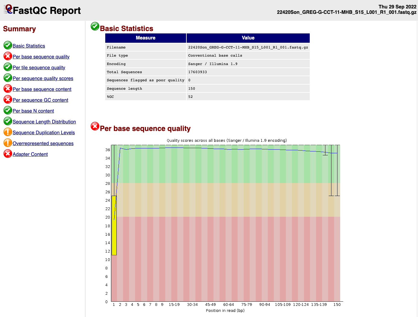
},EXAMPLE OF READS QUALITY BEFORE TRIMMING
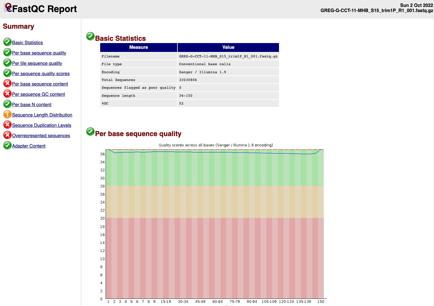
EXAMPLE OF READS QUALITY AFTER TRIMMING
We can see that the sequence length has changed and that the 5’ and 3’
end positions with lower quality have been removed.
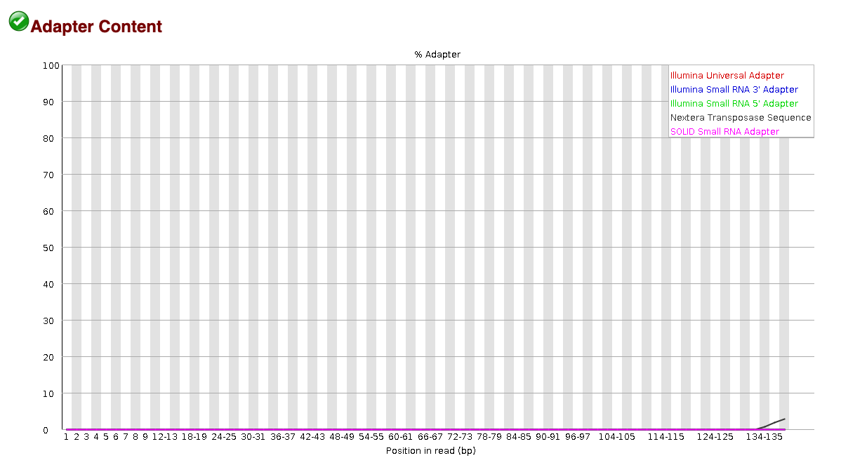
EXAMPLE OF READS QUALITY BEFORE TRIMMING
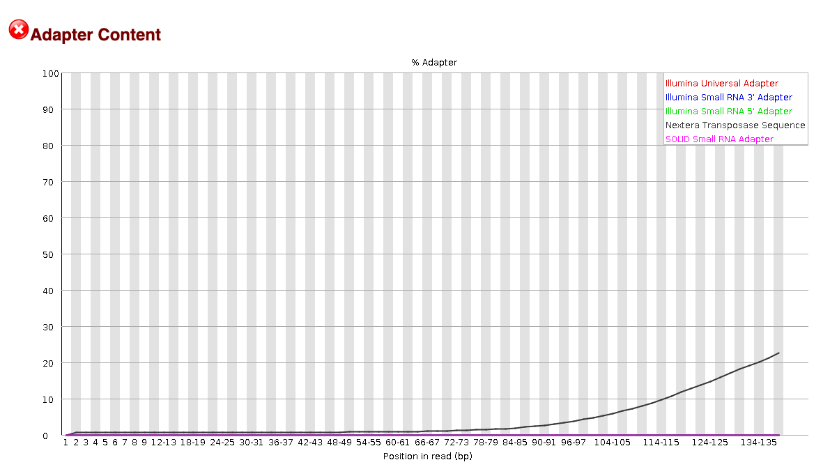
EXAMPLE OF READS QUALITY AFTER TRIMMING
We can see that most detected adapter sequences have been adequately
removed after trimming.
Non-target sequencing data
Contamination is likely to occur throughout various stages of experiments, including tissue acquisition, RNA extraction and library preparation. One can hope to reduces as much as possible its impact on the final sequencing data which can affect the success rate of reads mapping.
Screen for microbial contamination with Kaiju
We decided to screen for microbes sequences present in the trimmed
paired-end reads FASTQ.gz files using the tool Kaiju.
Kaiju translates metatranscriptomics sequencing reads into
six possible reading frames and searches for maximum exact matches of
amino acid sequences in a given annotation protein database.
We used the most extensive microbial database nr_euk
which encompass the subset of NCBI BLAST nr database containing all
proteins belonging to Archaea, Bacteria, Viruses, Fungi and microbial
Eukaryotes.
# enable proxy to allow compute node connection to internet
module load WebProxy

## Downloading the 2023-05-10 database from Kaiju webserver
wget --no-check-certificate https://kaiju-idx.s3.eu-central-1.amazonaws.com/2023/kaiju_db_nr_euk_2023-05-10.tgz
To run Kaiju we used the following
Snakemake rule:
########################################
# Snakefile rule
########################################

rule kaiju:
    input:
        database = KAIJUdir + "/kaiju_db_nr_euk.fmi",
        taxonid = KAIJUdir + "/nodes.dmp",
        taxonnames = KAIJUdir + "/names.dmp",
        trimmed_read1 = WORKDir + "/01-{species}-trimmed-tgalore/{locust}_1_val_1.fq.gz",
        trimmed_read2 = WORKDir + "/01-{species}-trimmed-tgalore/{locust}_2_val_2.fq.gz"
    output:
        kaijuout = WORKDir + "/KAIJU/{species}-kaiju/{locust}_kaiju.out",
        classification = WORKDir + "/KAIJU/{species}-kaiju/{locust}_kaiju.tsv"
    shell:
        """
        module purge
        ml GCC/8.3.0 OpenMPI/3.1.4 Kaiju/1.7.3-Python-3.7.4

        kaiju -z 12 -v \\
        -a greedy \\
        -f {input.database} \\
        -t {input.taxonid} \\
        -i {input.trimmed_read1} \\
        -j {input.trimmed_read2} \\
        -o {output.kaijuout}

        kaiju2table -v \\
        -t {input.taxonid} \\
        -n {input.taxonnames} \\
        -r phylum \\
        -o {output.classification} {output.kaijuout}
        """


########################################
# Parameters in the cluster.json file
########################################

    "kaiju":
    {
        "cpus-per-task" : 12,
        "partition" : "medium",
        "ntasks": 2,
        "mem" : "200G",
        "time": "0-12:00:00"
   },
-z 12: Sets the number of 12 CPU threads to use for parallel processing.-v: Enables verbose mode, which provides detailed output information as the program runs.-a greedy: Chooses thegreedyalgorithm for sequence alignment in Kaiju. This algorithm searches for the longest exact match in the database and allows for more sensitive, although potentially slower, matching compared to other options.-f {input.database}: Specifies the database file to use for classification, typically a precompiled.fmifile containing microbial or taxonomic protein sequences.-t {input.taxonid}: Points to the taxonomy node file (nodes.dmp), which Kaiju uses to assign taxonomic IDs based on the sequence matches. This file is part of the NCBI taxonomy data.-i {input.trimmed_read1}and-j {input.trimmed_read2}: Specifies the input FASTQ files for paired-end reads.-iis for the forward read file, and-jis for the reverse read file.-o {output.kaijuout}: Defines the output file for Kaiju results. This file contains the classifications and matches for each read.
Parameters for kaiju2table:
-n {input.taxonnames}: Points to the taxonomy names file (names.dmp), which Kaiju uses to convert taxonomic IDs into scientific names in the output table.-r phylum: Specifies the taxonomic rank at which results are summarized. Setting it tophylummeans that results will be grouped at the phylum level in the output table.-o {output.classification}: Specifies the output file for the generated classification table, where each row corresponds to a read’s classification and its taxonomic path to the specified rank (phylum).
The output produced here allows us to see the percentage of reads that map to unclassified (likely our locust host here) and the percentage of microbial contamination ranked in a phylum level.
Visualize the metatranscriptomics result
Kaiju output can be exported to be view in a interactive
and hierarchical multi-layered pie-charts using Krona. The
results are generated by a .html page. We followed the Kaiju tutorial
on the Github page:
########################################
# Snakefile rule
########################################

rule krona:
    input:
        kaijuout = WORKDir + "/KAIJU/{species}-kaiju/{locust}_kaiju.out",
        taxonid = KAIJUdir + "/nodes.dmp",
        taxonnames = KAIJUdir + "/names.dmp",
    output:
        conversion = WORKDir + "/KAIJU/{species}-kaiju/{locust}_krona.out",
        webreport = WORKDir + "/KAIJU/{species}-kaiju/{locust}_krona.html",
    shell:
        """
        module purge
        ml GCCcore/8.2.0 KronaTools/2.7.1

        kaiju2krona \\
        -t {input.taxonid} \\
        -n {input.taxonnames} \\
        -i {input.kaijuout} \\
        -o {output.conversion}

        ktImportText -o {output.webreport} {output.conversion}
        """

########################################
# Parameters in the cluster.json file
########################################

    "krona":
    {
        "cpus-per-task" : 2,
        "partition" : "short",
        "ntasks": 1,
        "mem" : "500M",
        "time": "0-0:10:00"
   },
-t {input.taxonid}: Specifies the taxonomy node file (nodes.dmp), which contains the hierarchical structure of taxonomic IDs. This file is used by Kaiju to organize and interpret taxonomic relationships for each classified read.-n {input.taxonnames}: Specifies the taxonomy names file (names.dmp), which maps taxonomic IDs to scientific names. This file allows Kaiju to output the actual names of taxa instead of numerical IDs.-i {input.kaijuout}: Indicates the input file with classification results generated by thekaijucommand. This file contains the taxonomic assignments for each read.-o {output.conversion}: Specifies the output file to be used as input for Krona. This file will be formatted to include taxonomic information that Krona can interpret, allowing for a hierarchical visualization of microbial content.-o {output.webreport}: Specifies the output HTML file that Krona will generate. This file will contain an interactive, multi-layered pie chart for visualizing the microbial classification data at different taxonomic levels.
Screen for microbial contamination with Kraken2
The combination of Kraken2 and Bracken is
another option to classify the reads compared to a database. Before
launching the snakemake, you will need to create a database:
# enable proxy to allow compute node connection to internet
module load WebProxy

## Downloading the Kraken database
wget --no-check-certificate https://genome-idx.s3.amazonaws.com/kraken/k2_core_nt_20240904.tar.gz
Then you can launch this Snakemake by referencing to
KRAKENDir.
########################################
# Snakefile rule
########################################

rule kraken2:
        input:
            trimmed_read1 = WORKDir + "/01-{species}-trimmed-tgalore/{locust}_1_val_1.fq.gz",
            trimmed_read2 = WORKDir + "/01-{species}-trimmed-tgalore/{locust}_2_val_2.fq.gz",
        params:
            report = WORKDir + "/KRAKEN2/{species}-kraken2/{locust}_report",
        output:
            taxoreport = WORKDir + "/KRAKEN2/{species}-kraken2/{locust}.kraken"),

        shell:
        """
        module purge
        ml GCC/11.2.0  OpenMPI/4.1.1 Kraken2/2.1.3

        kraken2 \\
        --use-names \\
        --threads 16 \\
        --db {KRAKENDir} \\
        --report {params.report} \\
        --gzip-compressed \\
        --paired {input.read1} {input.read2} > {output.taxoreport}
        """

rule braken:
        input:
            report = directory(WORKDir + "/KRAKEN2/{species}-kraken2/{locust}_report")
        output:
            taxonomy = WORKDir + "/KRAKEN2/{species}-kraken2/{locust}_GENUS.bracken")
        shell:
        """
        module purge
        ml GCCcore/10.3.0 Bracken/2.9

        bracken -v \\
        -d {KRAKENDir} \\
        -i {input.report} \\
        -l G \\
        -o {output.taxonomy}
        """

########################################
# Parameters in the cluster.json file
########################################
--paired {input.read1} {input.read2}: Specifies that the input data is paired-end sequencing reads, with{input.read1}as the forward read file and{input.read2}as the reverse read file.--gzip-compressed: Indicates that the input files are gzip-compressed, so Kraken2 will decompress them on the fly.--use-names: This option tells Kraken2 to display the taxonomic names in the output rather than just taxonomic IDs, making it easier to interpret the results directly.--db {KRAKENDir}: Specifies the path to the Kraken2 database, where{KRAKENDir}is a placeholder for the directory containing the database files. This database contains the reference sequences and taxonomy information Kraken2 uses to classify the reads.--report {params.report}: Defines the output file for the Kraken2 report, which summarizes the classification results, typically showing the percentage of reads classified at each taxonomic level.> {output.taxoreport}: Redirects the standard output of Kraken2 to a file,{output.taxoreport}, which will contain the detailed classification information for each read. This includes the assigned taxonomic classification and confidence scores.
sessionInfo()FALSE R version 4.4.1 (2024-06-14)
FALSE Platform: aarch64-apple-darwin20
FALSE Running under: macOS Sonoma 14.7
FALSE
FALSE Matrix products: default
FALSE BLAS: /Library/Frameworks/R.framework/Versions/4.4-arm64/Resources/lib/libRblas.0.dylib
FALSE LAPACK: /Library/Frameworks/R.framework/Versions/4.4-arm64/Resources/lib/libRlapack.dylib; LAPACK version 3.12.0
FALSE
FALSE locale:
FALSE [1] en_US.UTF-8/en_US.UTF-8/en_US.UTF-8/C/en_US.UTF-8/en_US.UTF-8
FALSE
FALSE time zone: Asia/Tokyo
FALSE tzcode source: internal
FALSE
FALSE attached base packages:
FALSE [1] stats graphics grDevices utils datasets methods base
FALSE
FALSE other attached packages:
FALSE [1] ggConvexHull_0.1.0 reshape2_1.4.4 ggthemes_5.1.0 plotly_4.10.4
FALSE [5] DT_0.33 lubridate_1.9.3 forcats_1.0.0 stringr_1.5.1
FALSE [9] dplyr_1.1.4 purrr_1.0.2 readr_2.1.5 tidyr_1.3.1
FALSE [13] tibble_3.2.1 ggplot2_3.5.1 tidyverse_2.0.0 rmdformats_1.0.4
FALSE [17] knitr_1.48
FALSE
FALSE loaded via a namespace (and not attached):
FALSE [1] gtable_0.3.6 xfun_0.49 bslib_0.8.0 htmlwidgets_1.6.4
FALSE [5] tzdb_0.4.0 vctrs_0.6.5 tools_4.4.1 generics_0.1.3
FALSE [9] fansi_1.0.6 highr_0.11 pkgconfig_2.0.3 data.table_1.16.2
FALSE [13] lifecycle_1.0.4 farver_2.1.2 compiler_4.4.1 git2r_0.35.0
FALSE [17] munsell_0.5.1 httpuv_1.6.15 htmltools_0.5.8.1 sass_0.4.9
FALSE [21] yaml_2.3.10 lazyeval_0.2.2 later_1.3.2 pillar_1.9.0
FALSE [25] crayon_1.5.3 jquerylib_0.1.4 whisker_0.4.1 cachem_1.1.0
FALSE [29] tidyselect_1.2.1 digest_0.6.37 stringi_1.8.4 bookdown_0.41
FALSE [33] labeling_0.4.3 rprojroot_2.0.4 fastmap_1.2.0 grid_4.4.1
FALSE [37] colorspace_2.1-1 cli_3.6.3 magrittr_2.0.3 utf8_1.2.4
FALSE [41] withr_3.0.2 scales_1.3.0 promises_1.3.0 timechange_0.3.0
FALSE [45] rmarkdown_2.28 httr_1.4.7 workflowr_1.7.1 hms_1.1.3
FALSE [49] evaluate_1.0.1 viridisLite_0.4.2 rlang_1.1.4 Rcpp_1.0.13
FALSE [53] glue_1.8.0 formatR_1.14 rstudioapi_0.17.1 jsonlite_1.8.9
FALSE [57] R6_2.5.1 plyr_1.8.9 fs_1.6.5