Last updated: 2024-11-18

Checks: 5 2

Knit directory: locust-comparative-genomics/

This reproducible R Markdown analysis was created with workflowr (version 1.7.1). The Checks tab describes the reproducibility checks that were applied when the results were created. The Past versions tab lists the development history.

R Markdown file: uncommitted changes

The R Markdown file has unstaged changes. To know which version of the R Markdown file created these results, you’ll want to first commit it to the Git repo. If you’re still working on the analysis, you can ignore this warning. When you’re finished, you can run wflow_publish to commit the R Markdown file and build the HTML.

Environment: empty

Great job! The global environment was empty. Objects defined in the global environment can affect the analysis in your R Markdown file in unknown ways. For reproduciblity it’s best to always run the code in an empty environment.

Seed: set.seed(20221025)

The command set.seed(20221025) was run prior to running the code in the R Markdown file. Setting a seed ensures that any results that rely on randomness, e.g. subsampling or permutations, are reproducible.

Session information: recorded

Great job! Recording the operating system, R version, and package versions is critical for reproducibility.

Cache: none

Nice! There were no cached chunks for this analysis, so you can be confident that you successfully produced the results during this run.

File paths: absolute

Using absolute paths to the files within your workflowr project makes it difficult for you and others to run your code on a different machine. Change the absolute path(s) below to the suggested relative path(s) to make your code more reproducible.

absolute	relative
/Users/maevatecher/Library/Mobile Documents/com_appleCloudDocs/Documents/GitHub/locust-comparative-genomics/data	data

Repository version: fe6dae9

Great! You are using Git for version control. Tracking code development and connecting the code version to the results is critical for reproducibility.

The results in this page were generated with repository version fe6dae9. See the Past versions tab to see a history of the changes made to the R Markdown and HTML files.

Note that you need to be careful to ensure that all relevant files for the analysis have been committed to Git prior to generating the results (you can use wflow_publish or wflow_git_commit). workflowr only checks the R Markdown file, but you know if there are other scripts or data files that it depends on. Below is the status of the Git repository when the results were generated:


Ignored files:
    Ignored:    .DS_Store
    Ignored:    .RData
    Ignored:    .Rhistory
    Ignored:    .Rproj.user/
    Ignored:    analysis/.DS_Store
    Ignored:    analysis/.Rhistory
    Ignored:    data/.DS_Store
    Ignored:    data/.Rhistory
    Ignored:    data/DEG-results/.DS_Store
    Ignored:    data/OLD/.DS_Store
    Ignored:    data/OLD/DEseq2_SCUBE_SCUBE_THORAX_STARnew_features/.DS_Store
    Ignored:    data/OLD/DEseq2_SGREG_SGREG_HEAD_STARnew_features/.DS_Store
    Ignored:    data/OLD/DEseq2_SGREG_SGREG_THORAX_STARnew_features/.DS_Store
    Ignored:    data/OLD/americana/.DS_Store
    Ignored:    data/OLD/americana/deg_counts/.DS_Store
    Ignored:    data/OLD/americana/deg_counts/STAR_newparams/.DS_Store
    Ignored:    data/OLD/cubense/deg_counts/STAR/cubense/featurecounts/
    Ignored:    data/OLD/cubense/deg_counts/STAR/gregaria/
    Ignored:    data/OLD/gregaria/.DS_Store
    Ignored:    data/OLD/gregaria/deg_counts/.DS_Store
    Ignored:    data/OLD/gregaria/deg_counts/STAR/.DS_Store
    Ignored:    data/OLD/gregaria/deg_counts/STAR/gregaria/.DS_Store
    Ignored:    data/OLD/gregaria/deg_counts/STAR_newparams/.DS_Store
    Ignored:    data/OLD/piceifrons/.DS_Store
    Ignored:    data/list/.DS_Store
    Ignored:    data/list/GO_Annotations/.DS_Store
    Ignored:    data/orthofinder/.DS_Store
    Ignored:    data/orthofinder/Orthogroups/.DS_Store
    Ignored:    figures/
    Ignored:    tables/

Untracked files:
    Untracked:  data/OLD/orthologs/Orthogroups_reprocessed.txt
    Untracked:  data/orthofinder/Orthogroups/Orthogroups_reprocessed.tsv
    Untracked:  data/orthofinder/Orthogroups/Orthogroups_reprocessed.txt

Unstaged changes:
    Modified:   analysis/3_go-enrichment.Rmd
    Modified:   analysis/3_wgcna-network.Rmd
    Modified:   data/orthofinder/Orthogroups/Orthogroups.txt

Note that any generated files, e.g. HTML, png, CSS, etc., are not included in this status report because it is ok for generated content to have uncommitted changes.

These are the previous versions of the repository in which changes were made to the R Markdown (analysis/3_go-enrichment.Rmd) and HTML (docs/3_go-enrichment.html) files. If you’ve configured a remote Git repository (see ?wflow_git_remote), click on the hyperlinks in the table below to view the files as they were in that past version.

File	Version	Author	Date	Message
Rmd	fe6dae9	Maeva TECHER	2024-11-18	changes ESA
html	fe6dae9	Maeva TECHER	2024-11-18	changes ESA
Rmd	3fa8e62	Maeva TECHER	2024-11-08	updated analysis
html	3fa8e62	Maeva TECHER	2024-11-08	updated analysis
Rmd	edb70fe	Maeva TECHER	2024-11-07	overlap and deg results created
html	edb70fe	Maeva TECHER	2024-11-07	overlap and deg results created
html	ba35b82	Maeva A. TECHER	2024-06-19	Build site.
html	d605bd3	Maeva A. TECHER	2024-05-16	Build site.
Rmd	9f04a80	Maeva A. TECHER	2024-05-16	wflow_publish("analysis/3_go-enrichment.Rmd")
html	d7b2c58	Maeva A. TECHER	2024-05-15	Build site.
Rmd	f5a78da	Maeva A. TECHER	2024-05-15	wflow_publish("analysis/3_go-enrichment.Rmd")
html	a32a56d	Maeva A. TECHER	2024-05-14	Build site.
Rmd	ebc0f04	Maeva A. TECHER	2024-05-14	wflow_publish("analysis/3_go-enrichment.Rmd")

Once we have shortlisted some genes of interest—whether they are obtained from top differentially expressed genes (DEGs), weighted gene co-expression network analysis (WGCNA) modules, or other comparative genomics analyses (e.g., signatures of selection, gene family expansion)—we want to determine if certain functions are enriched in our subset. For example, we hypothesize that although locusts have evolved similar traits, they may have diverged in their strategies to respond to the environment. Therefore, we expect to see DEGs involved in divergent biological processes, molecular function, and cellular components between S. gregaria, S. piceifrons and S. cancellata.

To test that, we need to look for Gene Ontology (GO) terms that can provide us a bird’s-eye of the related functions associated with our genes of interests.

1. Blast2Go file

To create the GO association file with each of our genome, we are using the paid version of OmicsBox with the integrated workflow Blast2Go. We details below our step-by-step with one Schistocerca genome, but followed the same process for all six RefSeq.

Step 1: Load Genome (fasta + GFF)

Step 2: Run Blast

We choose the More Sensitive mode of blastx from the Diamond Blast mode which allows to align large lists of nucelotide or protein sequences against up-to-date public sequence collections. Diamond Blast has a very similar accuracy compared to the NCBI Blast with a much higher throughput. All our association files were run against the Database (NR (2024-07-11)).

2. GO term enrichment

2.1. Load necessary libraries

library(topGO)
library(dplyr) 
library(ggplot2)
library(tidyr)
library(tibble)

# Define working directory and species
workDir <- "/Users/maevatecher/Library/Mobile Documents/com~apple~CloudDocs/Documents/GitHub/locust-comparative-genomics/data"
species <- "gregaria"

# Step 1: Load DESeq2 results for the species
deg_file <- file.path(workDir, "DEG-results", paste0("DESeq2_results_Head_", species, ".csv")) 
deg_data <- read.csv(deg_file, stringsAsFactors = FALSE)
names(deg_data)[names(deg_data) == "X"] <- "GeneID"

# Separate DEGs into upregulated and downregulated
upregulated_genes <- subset(deg_data, padj < 0.05 & log2FoldChange > 1)$GeneID
downregulated_genes <- subset(deg_data, padj < 0.05 & log2FoldChange < -1)$GeneID

# Load the custom annotation file
custom_annot_file <- file.path(workDir, "list/GO_Annotations", paste0("blast2go_", species, "_custom.txt")) 
custom_annot_df <- read.table(custom_annot_file, sep = "\t", header = TRUE, quote = "", fill = TRUE, stringsAsFactors = FALSE)

# Prepare gene-to-GO mapping for topGO
colnames(custom_annot_df) <- c("GeneID", "Description", "GO_Extended")
custom_annot_df <- custom_annot_df %>% 
    separate(GO_Extended, into = c("Category", "GO_ID", "GO_Term"), sep = " ", extra = "merge") %>%
    mutate(Category = substr(Category, 1, 1))

gene2GO <- custom_annot_df %>% 
  group_by(GeneID) %>% 
  summarize(GOterms = list(unique(GO_ID))) %>% 
  deframe()

# Function to run topGO analysis by ontology
run_topGO <- function(ontology, gene_set, gene2GO) {
  all_genes <- factor(as.integer(names(gene2GO) %in% gene_set), levels = c(0, 1))
  names(all_genes) <- names(gene2GO)
  GOdata <- new("topGOdata", ontology = ontology, allGenes = all_genes, annot = annFUN.gene2GO, gene2GO = gene2GO)
  resultFisher <- runTest(GOdata, algorithm = "classic", statistic = "fisher")
  GenTable(GOdata, classicFisher = resultFisher, orderBy = "classicFisher", topNodes = 10)
}

# Run topGO for each ontology category and regulation type
allRes_up_BP <- run_topGO("BP", upregulated_genes, gene2GO) %>% mutate(Regulation = "Upregulated", ontology = "BP")
allRes_up_MF <- run_topGO("MF", upregulated_genes, gene2GO) %>% mutate(Regulation = "Upregulated", ontology = "MF")
allRes_up_CC <- run_topGO("CC", upregulated_genes, gene2GO) %>% mutate(Regulation = "Upregulated", ontology = "CC")

allRes_down_BP <- run_topGO("BP", downregulated_genes, gene2GO) %>% mutate(Regulation = "Downregulated", ontology = "BP")
allRes_down_MF <- run_topGO("MF", downregulated_genes, gene2GO) %>% mutate(Regulation = "Downregulated", ontology = "MF")
allRes_down_CC <- run_topGO("CC", downregulated_genes, gene2GO) %>% mutate(Regulation = "Downregulated", ontology = "CC")

# Combine all results with ontology labels
allRes <- bind_rows(
  allRes_up_BP, allRes_up_MF, allRes_up_CC,
  allRes_down_BP, allRes_down_MF, allRes_down_CC
)

# Check if ontology is retained
head(allRes)

       GO.ID                          Term Annotated Significant Expected
1 GO:0055085       transmembrane transport       649          29    12.33
2 GO:0006810                     transport       987          36    18.75
3 GO:0051234 establishment of localization      1002          36    19.03
4 GO:0051179                  localization      1012          36    19.22
5 GO:0019310    inositol catabolic process         6           3     0.11
6 GO:0046164     alcohol catabolic process         7           3     0.13
  classicFisher  Regulation ontology
1       5.6e-06 Upregulated       BP
2       3.1e-05 Upregulated       BP
3       4.4e-05 Upregulated       BP
4       5.5e-05 Upregulated       BP
5       0.00013 Upregulated       BP
6       0.00022 Upregulated       BP

# Visualization with ggplot2
allRes$classicFisher <- as.numeric(as.character(allRes$classicFisher))
allRes$FoldEnrichment <- allRes$Significant / allRes$Expected

# Plot with ggplot2 using facet_wrap by ontology
ggplot(allRes, aes(x = reorder(Term, -log10(classicFisher)), y = -log10(classicFisher), size = Significant, color = FoldEnrichment)) +
    geom_point() +
    facet_wrap(~ ontology, scales = "free_y") +
    coord_flip() +
    labs(
        x = "GO Term", 
        y = "-log10(p-value)", 
        size = "Gene Count", 
        color = "Fold Enrichment", 
        title = "Top 10 Enriched GO Terms by Ontology",
        subtitle = "Head transcriptomes S. gregaria"
    ) +
    theme_minimal() +
    theme(
        plot.title = element_text(size = 16, face = "bold"),
        plot.subtitle = element_text(size = 12, face = "bold.italic"),
        axis.text.y = element_text(size = 8, face = "bold.italic", color = "black")
    ) +
    scale_size_continuous(range = c(3, 10)) +
    scale_color_viridis_c(option = "D")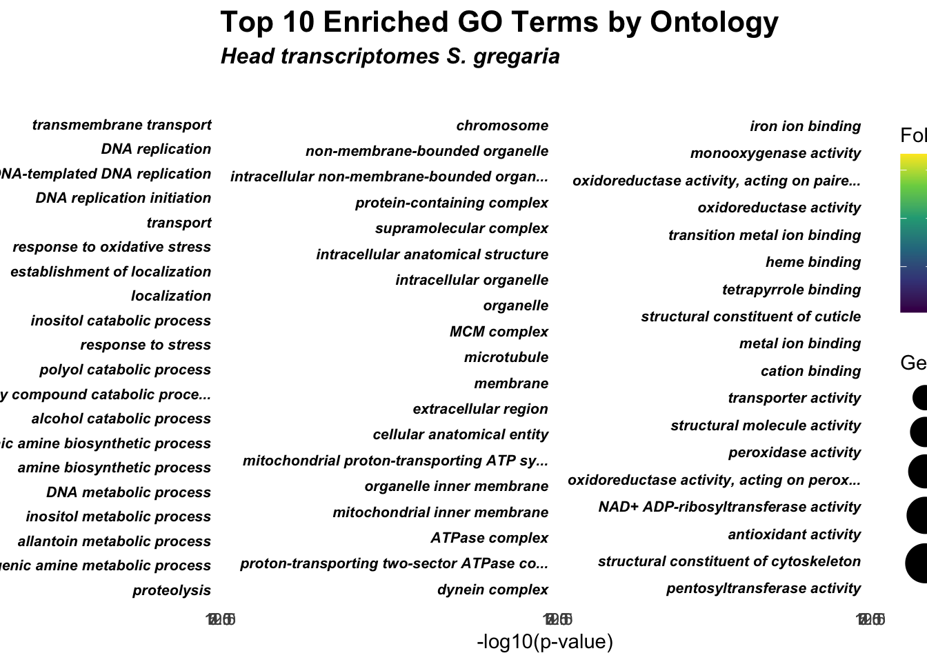

Version	Author	Date
fe6dae9	Maeva TECHER	2024-11-18
3fa8e62	Maeva TECHER	2024-11-08
edb70fe	Maeva TECHER	2024-11-07

# Plotting code up and downregulated
ggplot(allRes, aes(x = reorder(Term, -log10(classicFisher)), y = -log10(classicFisher), size = Significant, color = Regulation)) +
    geom_point() +
    facet_wrap(~ ontology, scales = "free_y") +
    coord_flip() +
    labs(
        x = "GO Term", 
        y = "-log10(p-value)", 
        size = "Gene Count", 
        color = "Regulation", 
        title = "Top 10 Enriched GO Terms by Ontology",
        subtitle = "Head transcriptomes S. gregaria"
    ) +
    theme_minimal() +
    theme(
        plot.title = element_text(size = 16, face = "bold"),
        plot.subtitle = element_text(size = 12, face = "italic"),
        axis.text.y = element_text(size = 8, face = "bold", color = "black")
    ) +
    scale_size_continuous(range = c(3, 10)) +
    scale_color_manual(values = c("Upregulated" = "red", "Downregulated" = "blue"))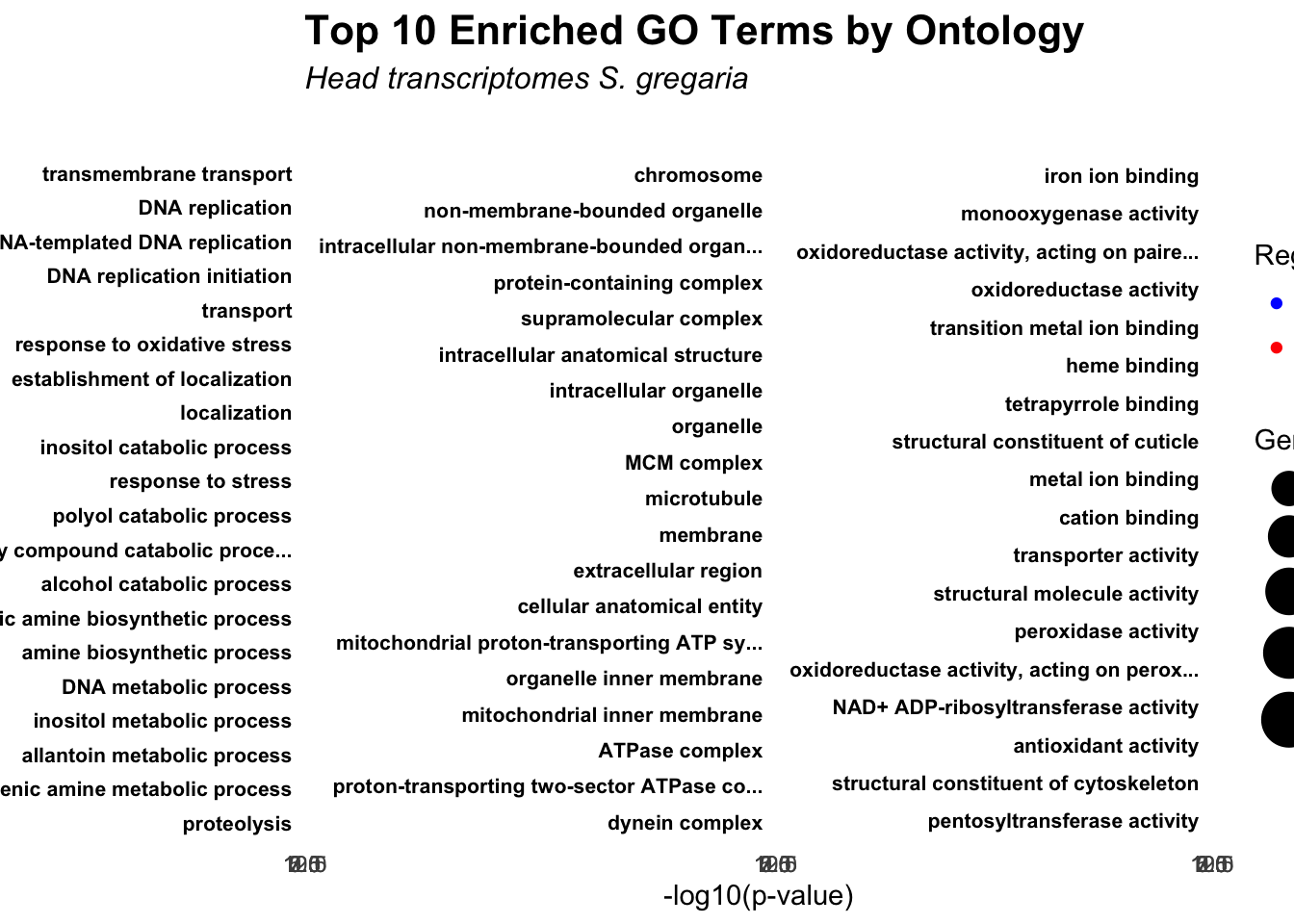

Version	Author	Date
fe6dae9	Maeva TECHER	2024-11-18
3fa8e62	Maeva TECHER	2024-11-08
edb70fe	Maeva TECHER	2024-11-07

# Bar Plot for top GO terms per ontology
ggplot(allRes, aes(x = FoldEnrichment, y = reorder(Term, FoldEnrichment), color = -log10(classicFisher), size = Significant)) +
    geom_point() +
    facet_wrap(~ ontology, scales = "free_y") +
    labs(
        x = "Fold Enrichment", 
        y = "GO Term", 
        color = "-log10(p-value)", 
        size = "Gene Count",
        title = "GO Term Enrichment: Fold Enrichment vs p-value"
    ) +
    theme_minimal() +
    theme(
        plot.title = element_text(size = 16, face = "bold"),
        plot.subtitle = element_text(size = 12, face = "bold.italic"),
        axis.text.y = element_text(size = 8, face = "bold", color = "black")
    ) +
    scale_fill_viridis_c(option = "C")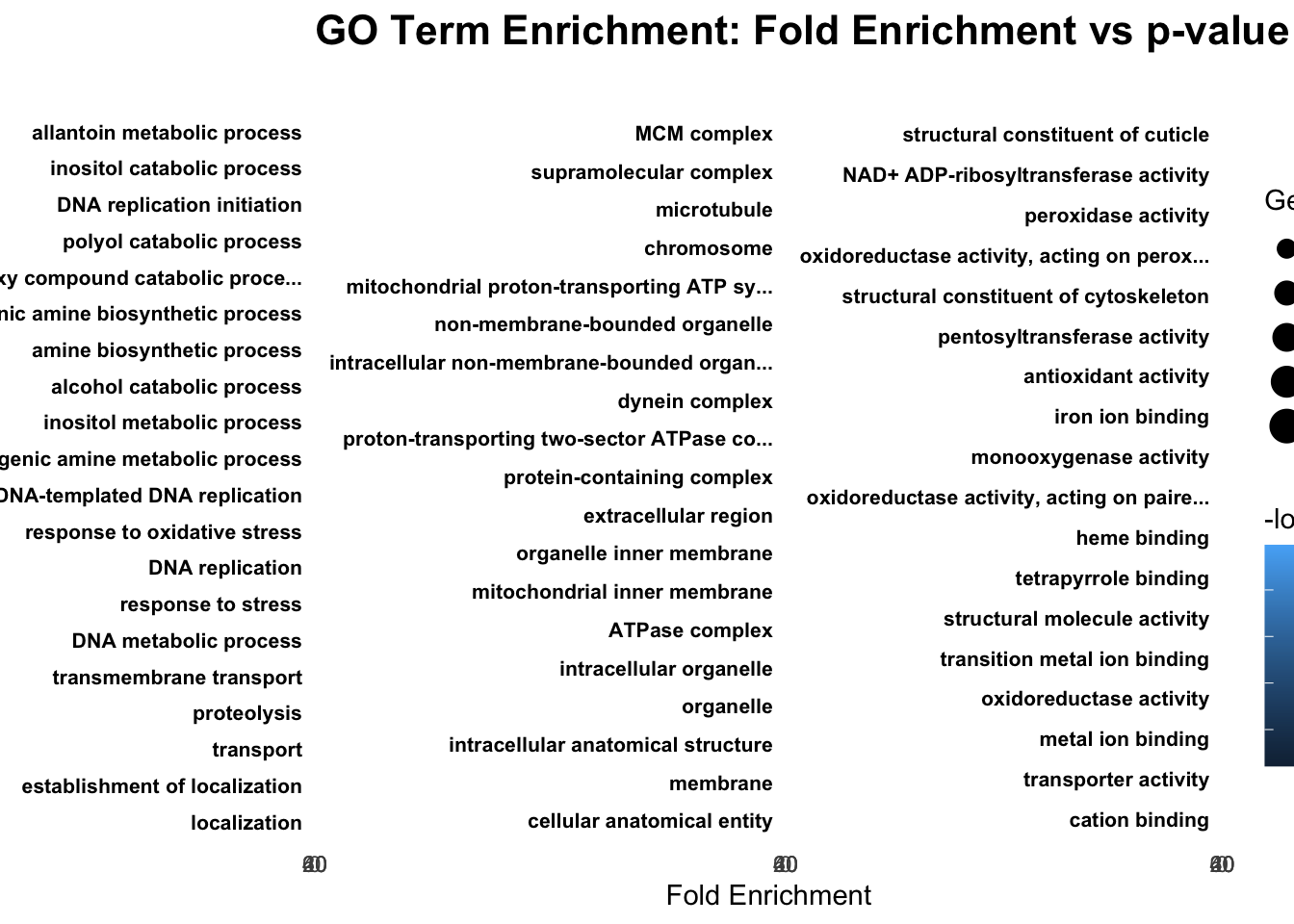

Version	Author	Date
fe6dae9	Maeva TECHER	2024-11-18

library(pheatmap)

# Aggregate data to ensure unique combinations of Term and ontology
# Keep the row with the smallest classicFisher value for each Term and ontology pair
heatmap_data <- allRes %>%
    group_by(Term, ontology) %>%
    slice_min(order_by = classicFisher, n = 1) %>%
    ungroup() %>%
    select(Term, ontology, classicFisher, Regulation) %>%
    spread(ontology, classicFisher) %>%
    column_to_rownames("Term")

# Separate the Regulation column from the numeric data for heatmap matrix
annotation <- data.frame(Regulation = heatmap_data$Regulation)
rownames(annotation) <- rownames(heatmap_data)

# Remove the Regulation column for matrix conversion
heatmap_matrix <- as.matrix(-log10(heatmap_data %>% select(-Regulation)))

# Replace any NAs with a high p-value and small values to avoid Inf
heatmap_matrix[is.na(heatmap_matrix)] <- -log10(1)  # Equivalent to a p-value of 1
heatmap_matrix[heatmap_matrix == -Inf] <- -log10(1e-300)  # Small positive value for zeroes

# Plot heatmap with annotation
pheatmap(heatmap_matrix, 
         cluster_rows = TRUE, 
         cluster_cols = FALSE, 
         color = colorRampPalette(c("white", "darkblue"))(50),
         annotation_row = annotation,
         main = "GO Term Enrichment Heatmap by Ontology",
         annotation_colors = list(Regulation = c("Upregulated" = "red", "Downregulated" = "blue")))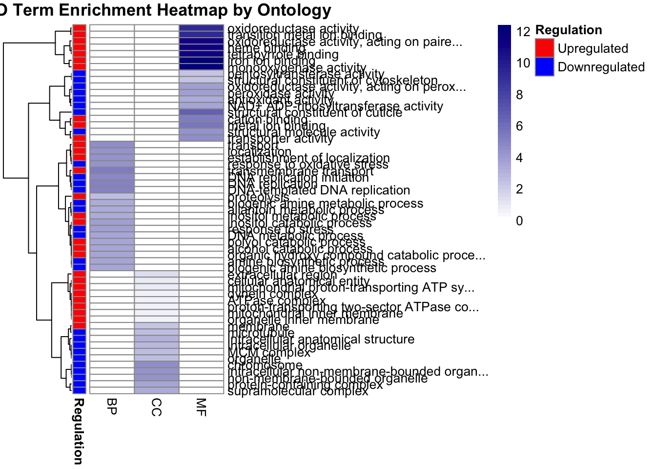

Version	Author	Date
fe6dae9	Maeva TECHER	2024-11-18

# Define working directory and species list
workDir <- "/Users/maevatecher/Library/Mobile Documents/com~apple~CloudDocs/Documents/GitHub/locust-comparative-genomics/data"
species_list <- c("gregaria", "piceifrons", "cancellata", "americana", "cubense", "nitens")

# Function to run the GO analysis for a given species
run_GO_analysis_for_species <- function(species) {
  # Load DESeq2 results for the species
  deg_file <- file.path(workDir, "DEG-results", paste0("DESeq2_results_Head_", species, ".csv"))
  deg_data <- read.csv(deg_file, stringsAsFactors = FALSE)
  names(deg_data)[names(deg_data) == "X"] <- "GeneID"
  
  # Separate DEGs into upregulated and downregulated
  upregulated_genes <- subset(deg_data, padj < 0.05 & log2FoldChange > 1)$GeneID
  downregulated_genes <- subset(deg_data, padj < 0.05 & log2FoldChange < -1)$GeneID
  
  # Load the custom annotation file
  custom_annot_file <- file.path(workDir, "list/GO_Annotations", paste0("blast2go_", species, "_custom.txt"))
  custom_annot_df <- read.table(custom_annot_file, sep = "\t", header = TRUE, quote = "", fill = TRUE, stringsAsFactors = FALSE)
  
  # Prepare gene-to-GO mapping for topGO
  colnames(custom_annot_df) <- c("GeneID", "Description", "GO_Extended")
  custom_annot_df <- custom_annot_df %>% 
    separate(GO_Extended, into = c("Category", "GO_ID", "GO_Term"), sep = " ", extra = "merge") %>%
    mutate(Category = substr(Category, 1, 1))
  
  gene2GO <- custom_annot_df %>%
    group_by(GeneID) %>%
    summarize(GOterms = list(unique(GO_ID))) %>%
    deframe()
  
  # Function to run topGO analysis by ontology
  run_topGO <- function(ontology, gene_set, gene2GO) {
    all_genes <- factor(as.integer(names(gene2GO) %in% gene_set), levels = c(0, 1))
    names(all_genes) <- names(gene2GO)
    GOdata <- new("topGOdata", ontology = ontology, allGenes = all_genes, annot = annFUN.gene2GO, gene2GO = gene2GO)
    resultFisher <- runTest(GOdata, algorithm = "classic", statistic = "fisher")
    GenTable(GOdata, classicFisher = resultFisher, orderBy = "classicFisher", topNodes = 10)
  }
  
  # Run topGO for each ontology category and regulation type
  allRes_up_BP <- run_topGO("BP", upregulated_genes, gene2GO) %>% mutate(Regulation = "Upregulated", ontology = "BP")
  allRes_up_MF <- run_topGO("MF", upregulated_genes, gene2GO) %>% mutate(Regulation = "Upregulated", ontology = "MF")
  allRes_up_CC <- run_topGO("CC", upregulated_genes, gene2GO) %>% mutate(Regulation = "Upregulated", ontology = "CC")
  
  allRes_down_BP <- run_topGO("BP", downregulated_genes, gene2GO) %>% mutate(Regulation = "Downregulated", ontology = "BP")
  allRes_down_MF <- run_topGO("MF", downregulated_genes, gene2GO) %>% mutate(Regulation = "Downregulated", ontology = "MF")
  allRes_down_CC <- run_topGO("CC", downregulated_genes, gene2GO) %>% mutate(Regulation = "Downregulated", ontology = "CC")
  
  # Combine all results with ontology labels
  allRes <- bind_rows(
    allRes_up_BP, allRes_up_MF, allRes_up_CC,
    allRes_down_BP, allRes_down_MF, allRes_down_CC
  )
  
  # Calculate FoldEnrichment and convert p-values
  allRes$classicFisher <- as.numeric(as.character(allRes$classicFisher))
  allRes$FoldEnrichment <- allRes$Significant / allRes$Expected
  
  # Export results for this species
  output_file <- file.path(workDir, "DEG-results", paste0("GO10_enrichment_Head_", species, "_custom.csv"))
  write.csv(allRes, output_file, row.names = FALSE)
  
  return(allRes)
}

# Name each element in species_list
names(species_list) <- species_list

# Run the analysis for each species
results_list <- lapply(species_list, run_GO_analysis_for_species)

# Combine all results into a single table if desired
combined_results <- bind_rows(results_list, .id = "Species")

# Define working directory and species list
workDir <- "/Users/maevatecher/Library/Mobile Documents/com~apple~CloudDocs/Documents/GitHub/locust-comparative-genomics/data"
species_list <- c("gregaria", "piceifrons", "cancellata", "americana", "cubense", "nitens")

# Function to run the GO analysis for a given species
run_GO_analysis_for_species <- function(species) {
  # Load DESeq2 results for the species
  deg_file <- file.path(workDir, "DEG-results", paste0("DESeq2_results_Thorax_", species, ".csv"))
  deg_data <- read.csv(deg_file, stringsAsFactors = FALSE)
  names(deg_data)[names(deg_data) == "X"] <- "GeneID"
  
  # Separate DEGs into upregulated and downregulated
  upregulated_genes <- subset(deg_data, padj < 0.05 & log2FoldChange > 1)$GeneID
  downregulated_genes <- subset(deg_data, padj < 0.05 & log2FoldChange < -1)$GeneID
  
  # Load the custom annotation file
  custom_annot_file <- file.path(workDir, "list/GO_Annotations", paste0("blast2go_", species, "_custom.txt"))
  custom_annot_df <- read.table(custom_annot_file, sep = "\t", header = TRUE, quote = "", fill = TRUE, stringsAsFactors = FALSE)
  
  # Prepare gene-to-GO mapping for topGO
  colnames(custom_annot_df) <- c("GeneID", "Description", "GO_Extended")
  custom_annot_df <- custom_annot_df %>% 
    separate(GO_Extended, into = c("Category", "GO_ID", "GO_Term"), sep = " ", extra = "merge") %>%
    mutate(Category = substr(Category, 1, 1))
  
  gene2GO <- custom_annot_df %>%
    group_by(GeneID) %>%
    summarize(GOterms = list(unique(GO_ID))) %>%
    deframe()
  
  # Function to run topGO analysis by ontology
  run_topGO <- function(ontology, gene_set, gene2GO) {
    all_genes <- factor(as.integer(names(gene2GO) %in% gene_set), levels = c(0, 1))
    names(all_genes) <- names(gene2GO)
    GOdata <- new("topGOdata", ontology = ontology, allGenes = all_genes, annot = annFUN.gene2GO, gene2GO = gene2GO)
    resultFisher <- runTest(GOdata, algorithm = "classic", statistic = "fisher")
    GenTable(GOdata, classicFisher = resultFisher, orderBy = "classicFisher", topNodes = 10)
  }
  
  # Run topGO for each ontology category and regulation type
  allRes_up_BP <- run_topGO("BP", upregulated_genes, gene2GO) %>% mutate(Regulation = "Upregulated", ontology = "BP")
  allRes_up_MF <- run_topGO("MF", upregulated_genes, gene2GO) %>% mutate(Regulation = "Upregulated", ontology = "MF")
  allRes_up_CC <- run_topGO("CC", upregulated_genes, gene2GO) %>% mutate(Regulation = "Upregulated", ontology = "CC")
  
  allRes_down_BP <- run_topGO("BP", downregulated_genes, gene2GO) %>% mutate(Regulation = "Downregulated", ontology = "BP")
  allRes_down_MF <- run_topGO("MF", downregulated_genes, gene2GO) %>% mutate(Regulation = "Downregulated", ontology = "MF")
  allRes_down_CC <- run_topGO("CC", downregulated_genes, gene2GO) %>% mutate(Regulation = "Downregulated", ontology = "CC")
  
  # Combine all results with ontology labels
  allRes <- bind_rows(
    allRes_up_BP, allRes_up_MF, allRes_up_CC,
    allRes_down_BP, allRes_down_MF, allRes_down_CC
  )
  
  # Calculate FoldEnrichment and convert p-values
  allRes$classicFisher <- as.numeric(as.character(allRes$classicFisher))
  allRes$FoldEnrichment <- allRes$Significant / allRes$Expected
  
  # Export results for this species
  output_file <- file.path(workDir, "DEG-results", paste0("GO10_enrichment_Thorax_", species, "_custom.csv"))
  write.csv(allRes, output_file, row.names = FALSE)
  
  return(allRes)
}

# Name each element in species_list
names(species_list) <- species_list

# Run the analysis for each species
results_list <- lapply(species_list, run_GO_analysis_for_species)

# Combine all results into a single table if desired
combined_results <- bind_rows(results_list, .id = "Species")

sessionInfo()

R version 4.4.1 (2024-06-14)
Platform: aarch64-apple-darwin20
Running under: macOS Sonoma 14.7

Matrix products: default
BLAS:   /Library/Frameworks/R.framework/Versions/4.4-arm64/Resources/lib/libRblas.0.dylib 
LAPACK: /Library/Frameworks/R.framework/Versions/4.4-arm64/Resources/lib/libRlapack.dylib;  LAPACK version 3.12.0

locale:
[1] en_US.UTF-8/en_US.UTF-8/en_US.UTF-8/C/en_US.UTF-8/en_US.UTF-8

time zone: America/Chicago
tzcode source: internal

attached base packages:
[1] stats4    stats     graphics  grDevices utils     datasets  methods  
[8] base     

other attached packages:
 [1] pheatmap_1.0.12      tibble_3.2.1         tidyr_1.3.1         
 [4] ggplot2_3.5.1        dplyr_1.1.4          topGO_2.56.0        
 [7] SparseM_1.84-2       GO.db_3.19.1         AnnotationDbi_1.66.0
[10] IRanges_2.38.1       S4Vectors_0.42.1     Biobase_2.64.0      
[13] graph_1.82.0         BiocGenerics_0.50.0 

loaded via a namespace (and not attached):
 [1] KEGGREST_1.44.1         gtable_0.3.6            xfun_0.49              
 [4] bslib_0.8.0             lattice_0.22-6          vctrs_0.6.5            
 [7] tools_4.4.1             generics_0.1.3          fansi_1.0.6            
[10] RSQLite_2.3.7           highr_0.11              blob_1.2.4             
[13] pkgconfig_2.0.3         RColorBrewer_1.1-3      lifecycle_1.0.4        
[16] GenomeInfoDbData_1.2.12 farver_2.1.2            compiler_4.4.1         
[19] stringr_1.5.1           git2r_0.35.0            Biostrings_2.72.1      
[22] munsell_0.5.1           httpuv_1.6.15           GenomeInfoDb_1.40.1    
[25] htmltools_0.5.8.1       sass_0.4.9              yaml_2.3.10            
[28] later_1.3.2             pillar_1.9.0            crayon_1.5.3           
[31] jquerylib_0.1.4         whisker_0.4.1           cachem_1.1.0           
[34] tidyselect_1.2.1        digest_0.6.37           stringi_1.8.4          
[37] purrr_1.0.2             labeling_0.4.3          rprojroot_2.0.4        
[40] fastmap_1.2.0           grid_4.4.1              colorspace_2.1-1       
[43] cli_3.6.3               magrittr_2.0.3          utf8_1.2.4             
[46] withr_3.0.2             scales_1.3.0            UCSC.utils_1.0.0       
[49] promises_1.3.0          bit64_4.5.2             rmarkdown_2.29         
[52] XVector_0.44.0          httr_1.4.7              matrixStats_1.4.1      
[55] bit_4.5.0               workflowr_1.7.1         png_0.1-8              
[58] memoise_2.0.1           evaluate_1.0.1          knitr_1.48             
[61] viridisLite_0.4.2       rlang_1.1.4             Rcpp_1.0.13-1          
[64] glue_1.8.0              DBI_1.2.3               rstudioapi_0.17.1      
[67] jsonlite_1.8.9          R6_2.5.1                fs_1.6.5               
[70] zlibbioc_1.50.0

Functional enrichment analysis

Maeva Techer

2024-11-18

1. Blast2Go file

Step 1: Load Genome (fasta + GFF)

Step 2: Run Blast

2. GO term enrichment

2.1. Load necessary libraries