Last updated: 2024-11-06

Checks: 5 2

Knit directory: locust-comparative-genomics/

This reproducible R Markdown analysis was created with workflowr (version 1.7.1). The Checks tab describes the reproducibility checks that were applied when the results were created. The Past versions tab lists the development history.

R Markdown file: uncommitted changes

The R Markdown file has unstaged changes. To know which version of the R Markdown file created these results, you’ll want to first commit it to the Git repo. If you’re still working on the analysis, you can ignore this warning. When you’re finished, you can run wflow_publish to commit the R Markdown file and build the HTML.

Environment: empty

Great job! The global environment was empty. Objects defined in the global environment can affect the analysis in your R Markdown file in unknown ways. For reproduciblity it’s best to always run the code in an empty environment.

Seed: set.seed(20221025)

The command set.seed(20221025) was run prior to running the code in the R Markdown file. Setting a seed ensures that any results that rely on randomness, e.g. subsampling or permutations, are reproducible.

Session information: recorded

Great job! Recording the operating system, R version, and package versions is critical for reproducibility.

Cache: none

Nice! There were no cached chunks for this analysis, so you can be confident that you successfully produced the results during this run.

File paths: absolute

Using absolute paths to the files within your workflowr project makes it difficult for you and others to run your code on a different machine. Change the absolute path(s) below to the suggested relative path(s) to make your code more reproducible.

absolute	relative
/Users/maevatecher/Library/Mobile Documents/com_appleCloudDocs/Documents/GitHub/locust-comparative-genomics/data	data

Repository version: 9fb9741

Great! You are using Git for version control. Tracking code development and connecting the code version to the results is critical for reproducibility.

The results in this page were generated with repository version 9fb9741. See the Past versions tab to see a history of the changes made to the R Markdown and HTML files.

Note that you need to be careful to ensure that all relevant files for the analysis have been committed to Git prior to generating the results (you can use wflow_publish or wflow_git_commit). workflowr only checks the R Markdown file, but you know if there are other scripts or data files that it depends on. Below is the status of the Git repository when the results were generated:


Ignored files:
    Ignored:    .DS_Store
    Ignored:    .RData
    Ignored:    .Rhistory
    Ignored:    .Rproj.user/
    Ignored:    analysis/.DS_Store
    Ignored:    analysis/.Rhistory
    Ignored:    analysis/figure/
    Ignored:    data/.DS_Store
    Ignored:    data/.Rhistory
    Ignored:    data/OLD/.DS_Store
    Ignored:    data/OLD/DEseq2_SCUBE_SCUBE_THORAX_STARnew_features/.DS_Store
    Ignored:    data/OLD/DEseq2_SGREG_SGREG_HEAD_STARnew_features/.DS_Store
    Ignored:    data/OLD/DEseq2_SGREG_SGREG_THORAX_STARnew_features/.DS_Store
    Ignored:    data/OLD/americana/.DS_Store
    Ignored:    data/OLD/americana/deg_counts/.DS_Store
    Ignored:    data/OLD/americana/deg_counts/STAR_newparams/.DS_Store
    Ignored:    data/OLD/cubense/deg_counts/STAR/cubense/featurecounts/
    Ignored:    data/OLD/cubense/deg_counts/STAR/gregaria/
    Ignored:    data/OLD/gregaria/.DS_Store
    Ignored:    data/OLD/gregaria/deg_counts/.DS_Store
    Ignored:    data/OLD/gregaria/deg_counts/STAR/.DS_Store
    Ignored:    data/OLD/gregaria/deg_counts/STAR/gregaria/.DS_Store
    Ignored:    data/OLD/gregaria/deg_counts/STAR_newparams/.DS_Store
    Ignored:    data/OLD/piceifrons/.DS_Store
    Ignored:    data/list/.DS_Store
    Ignored:    figures/
    Ignored:    tables/

Untracked files:
    Untracked:  VennDiagram.2024-11-06_18-59-50.734004.log
    Untracked:  VennDiagram.2024-11-06_18-59-50.787288.log
    Untracked:  VennDiagram.2024-11-06_18-59-50.81432.log
    Untracked:  VennDiagram.2024-11-06_19-03-11.527215.log
    Untracked:  VennDiagram.2024-11-06_19-03-11.572759.log
    Untracked:  VennDiagram.2024-11-06_19-03-11.602911.log
    Untracked:  analysis/VennDiagram.2024-11-06_18-58-51.746295.log
    Untracked:  analysis/VennDiagram.2024-11-06_18-58-51.858002.log
    Untracked:  analysis/VennDiagram.2024-11-06_18-58-51.932866.log
    Untracked:  data/03-americana-DESeq2-togregaria/
    Untracked:  data/03-cancellata-DESeq2-togregaria/
    Untracked:  data/03-cubense-DESeq2-togregaria/
    Untracked:  data/03-gregaria-DESeq2-togregaria/
    Untracked:  data/03-nitens-DESeq2-togregaria/
    Untracked:  data/03-piceifrons-DESeq2-togregaria/
    Untracked:  data/DEG-results/
    Untracked:  data/list/GO_Annotations/
    Untracked:  data/list/allspecies_geneid.csv
    Untracked:  data/list/allspecies_protein2geneid.tsv

Unstaged changes:
    Modified:   analysis/1_seq-data.Rmd
    Modified:   analysis/2_orthologs-prediction.Rmd
    Modified:   analysis/3_deseq2-results.Rmd
    Modified:   analysis/3_go-enrichment.Rmd
    Modified:   analysis/3_seq-data-qc.Rmd
    Deleted:    data/list/tx2gene.americana.csv

Note that any generated files, e.g. HTML, png, CSS, etc., are not included in this status report because it is ok for generated content to have uncommitted changes.

These are the previous versions of the repository in which changes were made to the R Markdown (analysis/3_go-enrichment.Rmd) and HTML (docs/3_go-enrichment.html) files. If you’ve configured a remote Git repository (see ?wflow_git_remote), click on the hyperlinks in the table below to view the files as they were in that past version.

File	Version	Author	Date	Message
html	ba35b82	Maeva A. TECHER	2024-06-19	Build site.
html	d605bd3	Maeva A. TECHER	2024-05-16	Build site.
Rmd	9f04a80	Maeva A. TECHER	2024-05-16	wflow_publish("analysis/3_go-enrichment.Rmd")
html	d7b2c58	Maeva A. TECHER	2024-05-15	Build site.
Rmd	f5a78da	Maeva A. TECHER	2024-05-15	wflow_publish("analysis/3_go-enrichment.Rmd")
html	a32a56d	Maeva A. TECHER	2024-05-14	Build site.
Rmd	ebc0f04	Maeva A. TECHER	2024-05-14	wflow_publish("analysis/3_go-enrichment.Rmd")

Once we have shortlisted some genes of interest—whether they are obtained from top differentially expressed genes (DEGs), weighted gene co-expression network analysis (WGCNA) modules, or other comparative genomics analyses (e.g., signatures of selection, gene family expansion)—we want to determine if certain functions are enriched in our subset. For example, we hypothesize that although locusts have evolved similar traits, they may have diverged in their strategies to respond to the environment. Therefore, we expect to see DEGs involved in divergent biological processes, molecular function, and cellular components between S. gregaria, S. piceifrons and S. cancellata.

To test that, we need to look for Gene Ontology (GO) terms that can provide us a bird’s-eye of the related functions associated with our genes of interests.

1. Blast2Go file

To create the GO association file with each of our genome, we are using the paid version of OmicsBox with the integrated workflow Blast2Go. We details below our step-by-step with one Schistocerca genome, but followed the same process for all six RefSeq.

Step 1: Load Genome (fasta + GFF)

Step 2: Run Blast

We choose the More Sensitive mode of blastx from the Diamond Blast mode which allows to align large lists of nucelotide or protein sequences against up-to-date public sequence collections. Diamond Blast has a very similar accuracy compared to the NCBI Blast with a much higher throughput. All our association files were run against the Database (NR (2024-07-11)).

2. GO term enrichment

2.1. Load necessary libraries

library(topGO)
library(dplyr) 
library(ggplot2)
library(tidyr)
library(tibble)

# Define working directory and species
workDir <- "/Users/maevatecher/Library/Mobile Documents/com~apple~CloudDocs/Documents/GitHub/locust-comparative-genomics/data"
species <- "gregaria"

# Step 1: Load and Filter Species-Specific Data
# Load DESeq2 results for the species
deg_file <- file.path(workDir, "DEG-results", paste0("DESeq2_results_head_", species, ".csv")) 
deg_data <- read.csv(deg_file, stringsAsFactors = FALSE)

# Filter for significant DEGs based on adjusted p-value and log2FoldChange threshold
sig_genes <- subset(deg_data, padj < 0.05 & abs(log2FoldChange) > 1)$GeneID

# Step 2: Map Genes to GO Terms
# Load the custom annotation file
custom_annot_file <- file.path(workDir, "list/GO_Annotations", paste0("blast2go_", species, "_custom.txt")) 
custom_annot_df <- read.table(custom_annot_file, sep = "\t", header = TRUE, quote = "", fill = TRUE, stringsAsFactors = FALSE)

# Rename columns and split `GO_Extended` into Category, GO_ID, and Term
colnames(custom_annot_df) <- c("GeneID", "Description", "GO_Extended")
custom_annot_df <- custom_annot_df %>% 
    separate(GO_Extended, into = c("Category", "GO_ID", "GO_Term"), sep = " ", extra = "merge") %>%
    mutate(Category = substr(Category, 1, 1))  # Ensures Category is one letter

# Group GO terms by GeneID to create gene-to-GO mapping for topGO
gene2GO <- custom_annot_df %>% 
  group_by(GeneID) %>% 
  summarize(GOterms = list(unique(GO_ID))) %>% 
  deframe()

# Step 3: Run GO Enrichment Analysis with topGO
# Create a vector of all genes, marking DEGs as TRUE
all_gene_names <- unique(names(gene2GO))  # All unique gene names in gene2GO 
all_genes <- factor(as.integer(all_gene_names %in% sig_genes), levels = c(0, 1)) 
names(all_genes) <- all_gene_names  # Set gene names as names for the factor

# Function to run topGO analysis by ontology
run_topGO <- function(ontology, all_genes, gene2GO) {
  GOdata <- new("topGOdata", ontology = ontology, allGenes = all_genes, annot = annFUN.gene2GO, gene2GO = gene2GO) 
  resultFisher <- runTest(GOdata, algorithm = "classic", statistic = "fisher") 
  GenTable(GOdata, classicFisher = resultFisher, orderBy = "classicFisher", topNodes = 10)
}

# Run topGO for each ontology category
allRes_BP <- run_topGO("BP", all_genes, gene2GO) 
allRes_MF <- run_topGO("MF", all_genes, gene2GO) 
allRes_CC <- run_topGO("CC", all_genes, gene2GO)

# Add ontology labels and combine results
allRes_BP$ontology <- "BP"
allRes_MF$ontology <- "MF" 
allRes_CC$ontology <- "CC" 
allRes <- rbind(allRes_BP, allRes_MF, allRes_CC)

# Step 4: Save GO enrichment results to a CSV file
output_file <- file.path(workDir, "DEG-results", paste0("GO_enrichment_head_", species, "_custom_top10.csv"))
write.csv(allRes, output_file, row.names = FALSE)

# Step 5: Visualization with ggplot2
# Prepare data for ggplot
allRes$classicFisher <- as.numeric(as.character(allRes$classicFisher))
allRes$FoldEnrichment <- allRes$Significant / allRes$Expected

# Plot with ggplot2 using facet_wrap by ontology
ggplot(allRes, aes(x = reorder(Term, -log10(classicFisher)), y = -log10(classicFisher), size = Significant, color = FoldEnrichment)) +
    geom_point() +
    facet_wrap(~ ontology, scales = "free_y") +
    coord_flip() +
    labs(
        x = "GO Term", 
        y = "-log10(p-value)", 
        size = "Gene Count", 
        color = "Fold Enrichment", 
        title = "Top 10 Enriched GO Terms by Ontology",
        subtitle = "Head transcriptomes S. gregaria"
    ) +
    theme_minimal() +
    theme(
        plot.title = element_text(size = 16, face = "bold"),
        plot.subtitle = element_text(size = 12, face = "bold.italic"),
        axis.text.y = element_text(size = 8, face = "bold.italic", color = "black")
    ) +
    scale_size_continuous(range = c(3, 10)) +
    scale_color_viridis_c(option = "D")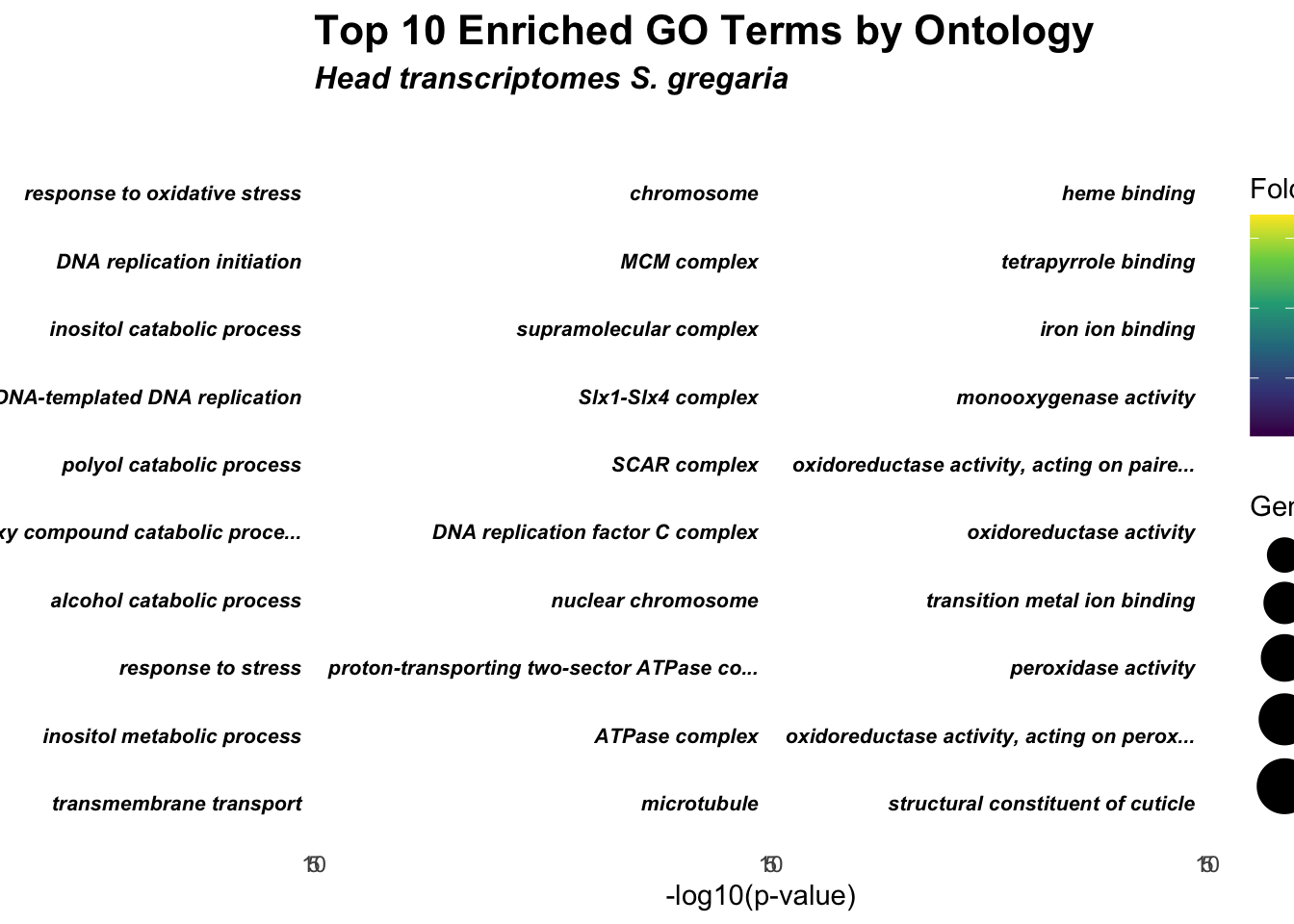

# Bar Plot for top GO terms per ontology
ggplot(allRes, aes(x = reorder(Term, -log10(classicFisher)), y = -log10(classicFisher), fill = ontology)) +
    geom_bar(stat = "identity", position = "dodge") +
    facet_wrap(~ ontology, scales = "free_y") +
    coord_flip() +
    labs(
        x = "GO Term", 
        y = "-log10(p-value)", 
        fill = "Ontology", 
        title = "Top 10 Enriched GO Terms by Ontology (Bar Plot)",
        subtitle = "Head transcriptomes S. gregaria"
    ) +
    theme_minimal() +
    theme(
        plot.title = element_text(size = 16, face = "bold"),
        plot.subtitle = element_text(size = 12, face = "bold.italic"),
        axis.text.y = element_text(size = 8, face = "bold", color = "black")
    ) +
    scale_fill_viridis_d(option = "C")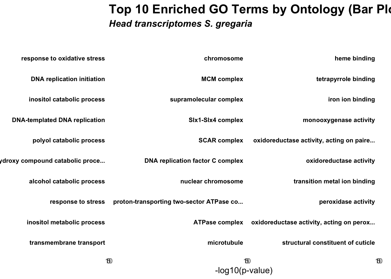

# Define working directory and species
workDir <- "/Users/maevatecher/Library/Mobile Documents/com~apple~CloudDocs/Documents/GitHub/locust-comparative-genomics/data"
species <- "gregaria"

# Step 1: Load DESeq2 results for the species
deg_file <- file.path(workDir, "DEG-results", paste0("DESeq2_results_head_", species, ".csv")) 
deg_data <- read.csv(deg_file, stringsAsFactors = FALSE)

# Filter significant DEGs based on adjusted p-value and log2FoldChange threshold
deg_data <- deg_data %>% mutate(
    Regulation = case_when(
        padj < 0.05 & log2FoldChange > 1 ~ "Upregulated",
        padj < 0.05 & log2FoldChange < -1 ~ "Downregulated",
        TRUE ~ "Not Significant"
    )
)

# Step 2: Select Top 10 Upregulated and Downregulated Genes with Descriptions
top10_up <- deg_data %>% filter(Regulation == "Upregulated") %>%
    arrange(desc(log2FoldChange)) %>%
    slice(1:10)

top10_down <- deg_data %>% filter(Regulation == "Downregulated") %>%
    arrange(log2FoldChange) %>%
    slice(1:10)

# Combine top upregulated and downregulated genes with descriptions
top_genes <- bind_rows(top10_up, top10_down) %>%
    select(GeneID, log2FoldChange, Description, Regulation) %>%
    arrange(desc(log2FoldChange))

# Step 3: Generate the Bar Plot
ggplot(top_genes, aes(x = reorder(paste(GeneID, Description, sep = ": "), log2FoldChange), y = log2FoldChange, fill = Regulation)) +
    geom_bar(stat = "identity", position = "dodge") +
    coord_flip() +
    labs(
        x = "Gene (Description)", 
        y = "Log2 Fold Change", 
        fill = "Regulation",
        title = "Top 10 Upregulated and Downregulated Genes",
        subtitle = "Head transcriptomes S. gregaria"
    ) +
    theme_minimal() +
    theme(
        plot.title = element_text(size = 16, face = "bold"),
        plot.subtitle = element_text(size = 12, face = "italic"),
        axis.text.y = element_text(size = 8, face = "bold", color = "black")
    ) +
    scale_fill_manual(values = c("Upregulated" = "red", "Downregulated" = "blue"))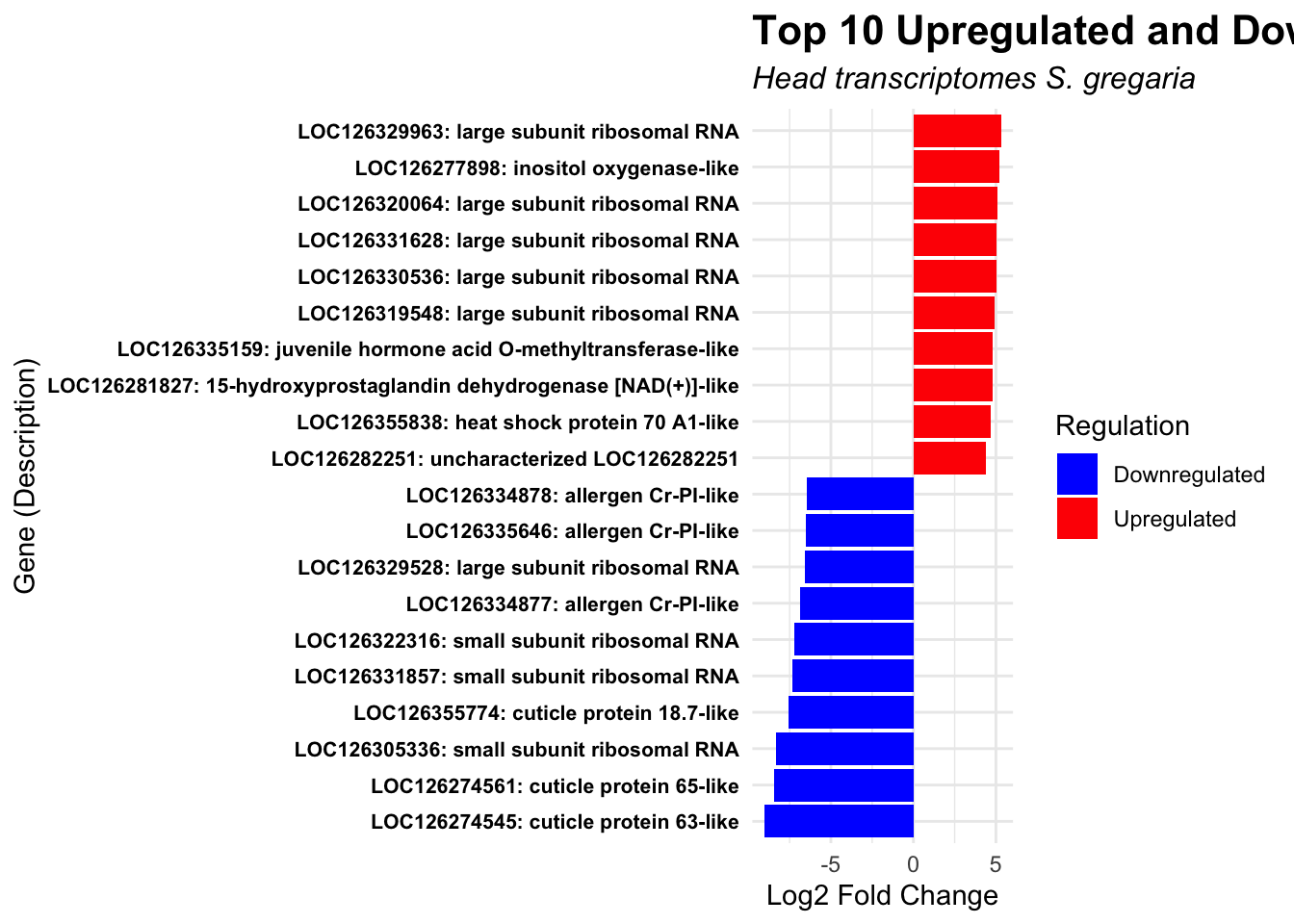

# SCATTER
# Load necessary libraries 
library(dplyr) 
library(ggplot2)

# Define working directory and species
workDir <- "/Users/maevatecher/Library/Mobile Documents/com~apple~CloudDocs/Documents/GitHub/locust-comparative-genomics/data"
species <- "gregaria"

# Load DESeq2 results for head and thorax
head_file <- file.path(workDir, "DEG-results", paste0("DESeq2_results_head_", species, ".csv"))
thorax_file <- file.path(workDir, "DEG-results", paste0("DESeq2_results_thorax_", species, ".csv"))

head_data <- read.csv(head_file, stringsAsFactors = FALSE)
thorax_data <- read.csv(thorax_file, stringsAsFactors = FALSE)

# Filter significant DEGs for both head and thorax
head_sig_genes <- head_data %>%
    filter(padj < 0.05 & abs(log2FoldChange) > 1) %>%
    select(GeneID, log2FoldChange, padj)

thorax_sig_genes <- thorax_data %>%
    filter(padj < 0.05 & abs(log2FoldChange) > 1) %>%
    select(GeneID, log2FoldChange, padj)

# Find overlapping genes based on GeneID
overlapping_genes <- inner_join(head_sig_genes, thorax_sig_genes, by = "GeneID", suffix = c("_head", "_thorax"))

# Save the overlapping genes to a CSV file
output_file <- file.path(workDir, "DEG-results", paste0("overlapping_genes_head_thorax_", species, ".csv"))
write.csv(overlapping_genes, output_file, row.names = FALSE)

# Plot overlapping genes with scatter plot
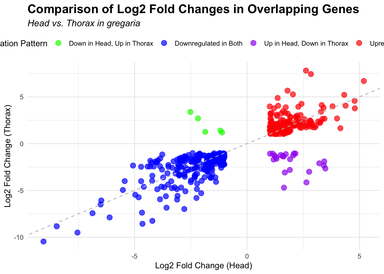
ggplot(overlapping_genes, aes(x = log2FoldChange_head, y = log2FoldChange_thorax)) +
    geom_point(aes(color = case_when(
        log2FoldChange_head > 0 & log2FoldChange_thorax > 0 ~ "Upregulated in Both",
        log2FoldChange_head < 0 & log2FoldChange_thorax < 0 ~ "Downregulated in Both",
        log2FoldChange_head > 0 & log2FoldChange_thorax < 0 ~ "Up in Head, Down in Thorax",
        log2FoldChange_head < 0 & log2FoldChange_thorax > 0 ~ "Down in Head, Up in Thorax"
    )), size = 3, alpha = 0.7) +  # Added alpha for transparency
    geom_abline(slope = 1, intercept = 0, linetype = "dashed", color = "gray") +
    labs(
        x = "Log2 Fold Change (Head)", 
        y = "Log2 Fold Change (Thorax)", 
        color = "Regulation Pattern", 
        title = "Comparison of Log2 Fold Changes in Overlapping Genes", 
        subtitle = paste("Head vs. Thorax in", species)
    ) +
    theme_minimal() + 
    theme(
        plot.title = element_text(size = 16, face = "bold"), 
        plot.subtitle = element_text(size = 12, face = "italic"), 
        legend.position = "top"
    ) +
    scale_color_manual(values = c(
        "Upregulated in Both" = "red", 
        "Downregulated in Both" = "blue", 
        "Up in Head, Down in Thorax" = "purple", 
        "Down in Head, Up in Thorax" = "green"
    ))

# VENN

# Load necessary libraries
library(VennDiagram)
library(gridExtra)
library(grid)

# Define working directory and species
workDir <- "/Users/maevatecher/Library/Mobile Documents/com~apple~CloudDocs/Documents/GitHub/locust-comparative-genomics/data"
species <- "gregaria"

# Load DESeq2 results for head and thorax
head_file <- file.path(workDir, "DEG-results", paste0("DESeq2_results_head_", species, ".csv"))
thorax_file <- file.path(workDir, "DEG-results", paste0("DESeq2_results_thorax_", species, ".csv"))

head_data <- read.csv(head_file, stringsAsFactors = FALSE)
thorax_data <- read.csv(thorax_file, stringsAsFactors = FALSE)

# Filter significant DEGs for both head and thorax
head_sig_genes <- head_data %>%
    filter(padj < 0.05 & abs(log2FoldChange) > 1) %>%
    select(GeneID)

thorax_sig_genes <- thorax_data %>%
    filter(padj < 0.05 & abs(log2FoldChange) > 1) %>%
    select(GeneID)


# Separate upregulated and downregulated genes
head_up <- head_data %>%
    filter(padj < 0.05 & log2FoldChange > 1) %>%
    select(GeneID)

head_down <- head_data %>%
    filter(padj < 0.05 & log2FoldChange < -1) %>%
    select(GeneID)

thorax_up <- thorax_data %>%
    filter(padj < 0.05 & log2FoldChange > 1) %>%
    select(GeneID)

thorax_down <- thorax_data %>%
    filter(padj < 0.05 & log2FoldChange < -1) %>%
    select(GeneID)

# Prepare data for Venn diagrams
venn_data_all <- list(
    Head = head_sig_genes$GeneID,
    Thorax = thorax_sig_genes$GeneID
)

venn_data_up <- list(
    Head = head_up$GeneID,
    Thorax = thorax_up$GeneID
)

venn_data_down <- list(
    Head = head_down$GeneID,
    Thorax = thorax_down$GeneID
)

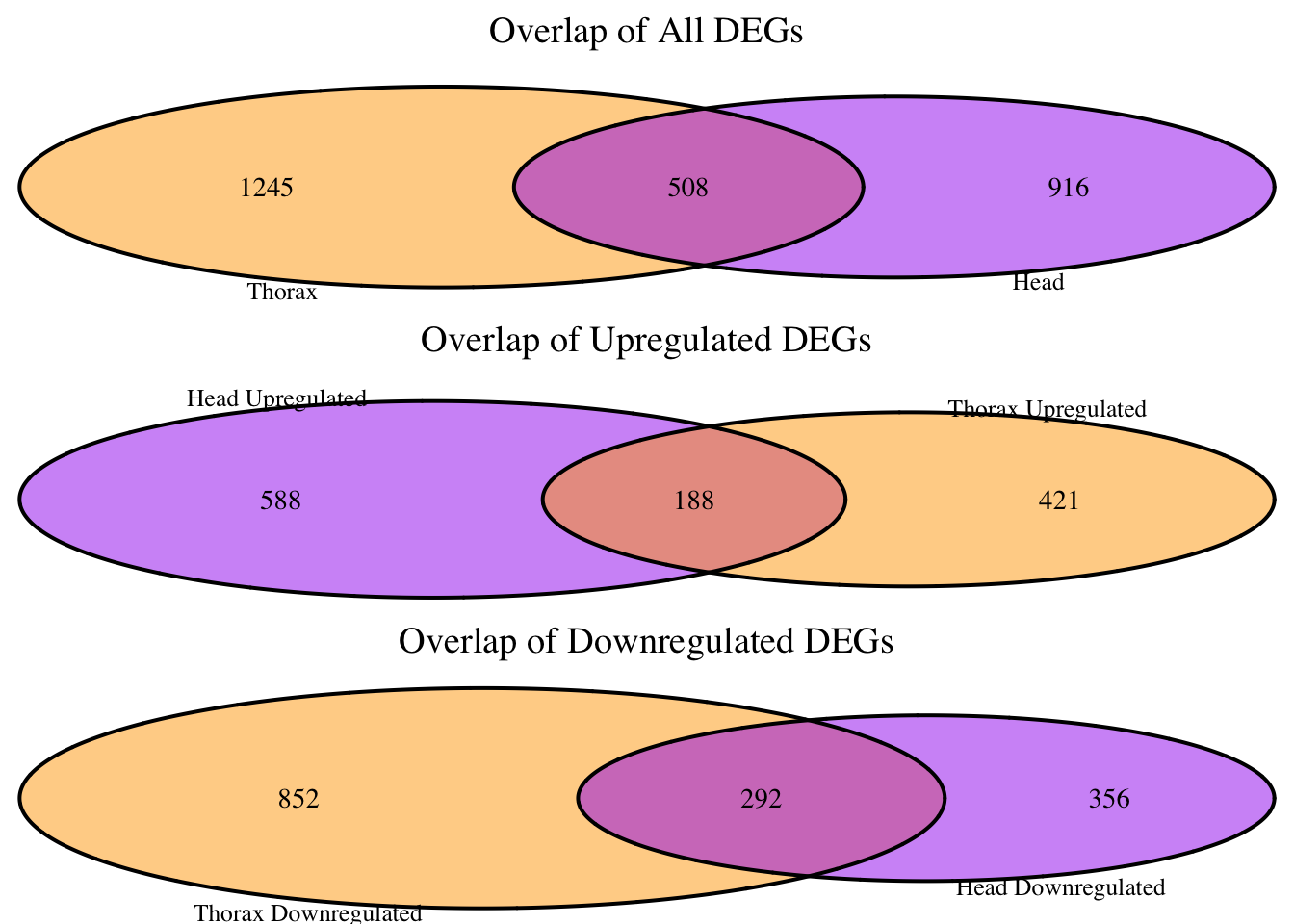
# Generate Venn diagrams with specific colors and arranged properly
venn_all <- venn.diagram(
    x = venn_data_all, 
    category.names = c("Head", "Thorax"), 
    filename = NULL, 
    output = TRUE, 
    fill = c("purple", "orange"),  # Set colors for head and thorax
    alpha = 0.5, 
    cex = 0.9,  # Smaller text for numbers
    cat.cex = 0.8,  # Smaller legend labels
    cat.pos = c(-20, 20), 
    cat.dist = c(0.02, 0.02),  # Closer distance between category labels and circles
    main = "Overlap of All DEGs", 
    main.cex = 1.2  # Smaller title
)

venn_up <- venn.diagram(
    x = venn_data_up, 
    category.names = c("Head Upregulated", "Thorax Upregulated"), 
    filename = NULL, 
    output = TRUE, 
    fill = c("purple", "orange"),  # Same color scheme
    alpha = 0.5, 
    cex = 0.9, 
    cat.cex = 0.8, 
    cat.pos = c(-20, 20), 
    cat.dist = c(0.02, 0.02), 
    main = "Overlap of Upregulated DEGs", 
    main.cex = 1.2
)

venn_down <- venn.diagram(
    x = venn_data_down, 
    category.names = c("Head Downregulated", "Thorax Downregulated"), 
    filename = NULL, 
    output = TRUE, 
    fill = c("purple", "orange"),  # Same color scheme
    alpha = 0.5, 
    cex = 0.9, 
    cat.cex = 0.8, 
    cat.pos = c(-20, 20), 
    cat.dist = c(0.02, 0.02), 
    main = "Overlap of Downregulated DEGs", 
    main.cex = 1.2
)

# Arrange the Venn diagrams in one column
grid.arrange(
    grobTree(venn_all), 
    grobTree(venn_up), 
    grobTree(venn_down), 
    ncol = 1
)

# HEATMAP

# Load necessary libraries
library(dplyr)
library(ggplot2)
library(pheatmap)
library(tidyr)

# Define working directory and species
workDir <- "/Users/maevatecher/Library/Mobile Documents/com~apple~CloudDocs/Documents/GitHub/locust-comparative-genomics/data"
species <- "gregaria"

# Load DESeq2 results for head and thorax
head_file <- file.path(workDir, "DEG-results", paste0("DESeq2_results_head_", species, ".csv"))
thorax_file <- file.path(workDir, "DEG-results", paste0("DESeq2_results_thorax_", species, ".csv"))

head_data <- read.csv(head_file, stringsAsFactors = FALSE)
thorax_data <- read.csv(thorax_file, stringsAsFactors = FALSE)

# Filter for significant DEGs and select top 40 upregulated and downregulated genes for each tissue
head_up <- head_data %>%
    filter(padj < 0.05 & log2FoldChange > 1) %>%
    arrange(desc(log2FoldChange)) %>%
    slice(1:40)

head_down <- head_data %>%
    filter(padj < 0.05 & log2FoldChange < -1) %>%
    arrange(log2FoldChange) %>%
    slice(1:40)

thorax_up <- thorax_data %>%
    filter(padj < 0.05 & log2FoldChange > 1) %>%
    arrange(desc(log2FoldChange)) %>%
    slice(1:40)

thorax_down <- thorax_data %>%
    filter(padj < 0.05 & log2FoldChange < -1) %>%
    arrange(log2FoldChange) %>%
    slice(1:40)

# Combine data and prepare for heatmap
heatmap_data <- bind_rows(
    head_up %>% mutate(Tissue = "Head", Regulation = "Upregulated"),
    head_down %>% mutate(Tissue = "Head", Regulation = "Downregulated"),
    thorax_up %>% mutate(Tissue = "Thorax", Regulation = "Upregulated"),
    thorax_down %>% mutate(Tissue = "Thorax", Regulation = "Downregulated")
) %>%
    select(GeneID, log2FoldChange, Tissue, Regulation)

# Spread data to have tissues as columns for heatmap format
heatmap_matrix <- heatmap_data %>%
    pivot_wider(names_from = c("Tissue", "Regulation"), values_from = log2FoldChange, values_fill = list(log2FoldChange = 0)) %>%
    column_to_rownames("GeneID") %>%
    as.matrix()

# Create combined log2FoldChange values for Head and Thorax
combined_matrix <- data.frame(
    GeneID = rownames(heatmap_matrix),
    Combined_Head = rowMeans(heatmap_matrix[, c("Head_Upregulated", "Head_Downregulated")], na.rm = TRUE),
    Combined_Thorax = rowMeans(heatmap_matrix[, c("Thorax_Upregulated", "Thorax_Downregulated")], na.rm = TRUE)
)

# Set rownames for combined matrix
rownames(combined_matrix) <- combined_matrix$GeneID
combined_matrix <- combined_matrix[, -1]  # Remove GeneID column

# Define breaks for legend
legend_breaks <- seq(-2, 2, by = 1)
legend_labels <- c("Downregulated", "No change", "Upregulated")

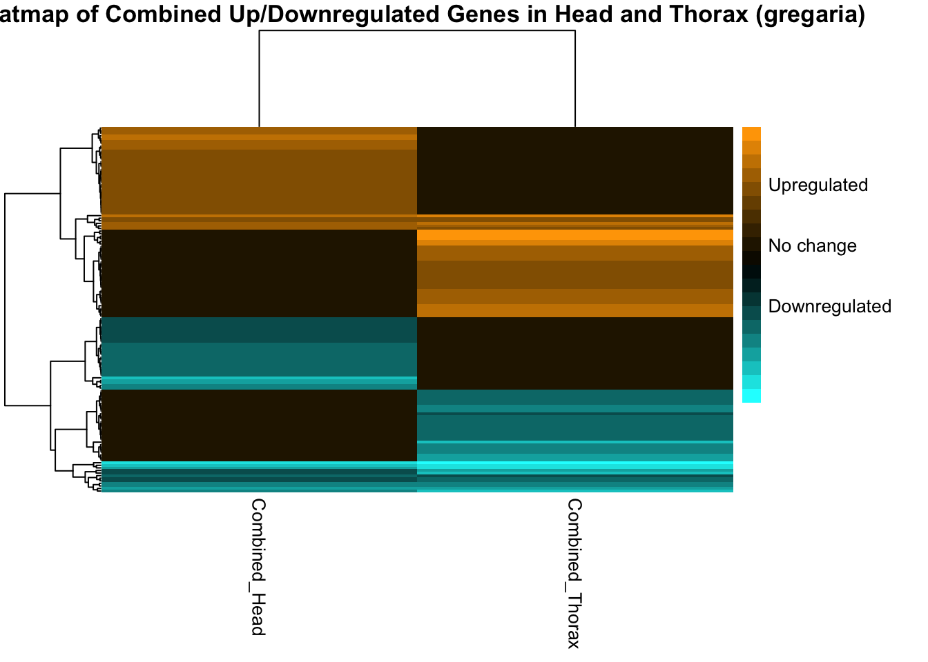
# Generate heatmap with pheatmap
pheatmap(
    combined_matrix,
    color = colorRampPalette(c("cyan", "black", "orange"))(20),
    cluster_rows = TRUE,
    cluster_cols = TRUE,
    show_rownames = FALSE,  # Remove LOCUS labels
    show_colnames = TRUE,
    main = paste("Heatmap of Combined Up/Downregulated Genes in Head and Thorax (", species, ")", sep = ""),
    legend_breaks = legend_breaks[legend_breaks %in% c(-2, 0, 2)],  # Ensure we only use the breaks we have labels for
    legend_labels = c("Downregulated", "No change", "Upregulated"),  # This corresponds to the colors
    fontsize = 10  # Adjust font size for better readability
)

## HEATMAP ALL

# Load necessary libraries
library(reshape2)
library(ggplot2)

# Assuming head_sig_genes and thorax_sig_genes are already defined

# Filter significant DEGs for both head and thorax
head_sig_genes <- head_data %>%
    filter(padj < 0.05 & abs(log2FoldChange) > 1) %>%
    select(GeneID, log2FoldChange, padj)

thorax_sig_genes <- thorax_data %>%
    filter(padj < 0.05 & abs(log2FoldChange) > 1) %>%
    select(GeneID, log2FoldChange, padj)

# Combine the data with appropriate log2FoldChange values for both head and thorax
heatmap_data <- merge(head_sig_genes, thorax_sig_genes, by = "GeneID", suffixes = c("_head", "_thorax"))

# Create a melted dataframe for heatmap plotting
heatmap_long <- melt(heatmap_data, id.vars = "GeneID", 
                     measure.vars = c("log2FoldChange_head", "log2FoldChange_thorax"), 
                     variable.name = "Tissue", 
                     value.name = "Log2FoldChange")

# Create a new column for coloring based on tissue
heatmap_long$Tissue <- factor(heatmap_long$Tissue, levels = 
                               c("log2FoldChange_head", "log2FoldChange_thorax"), 
                               labels = c("Head", "Thorax"))

# Adjust the color scale based on Log2 Fold Change
heatmap_long$Color <- ifelse(heatmap_long$Log2FoldChange > 0, "Upregulated", "Downregulated")

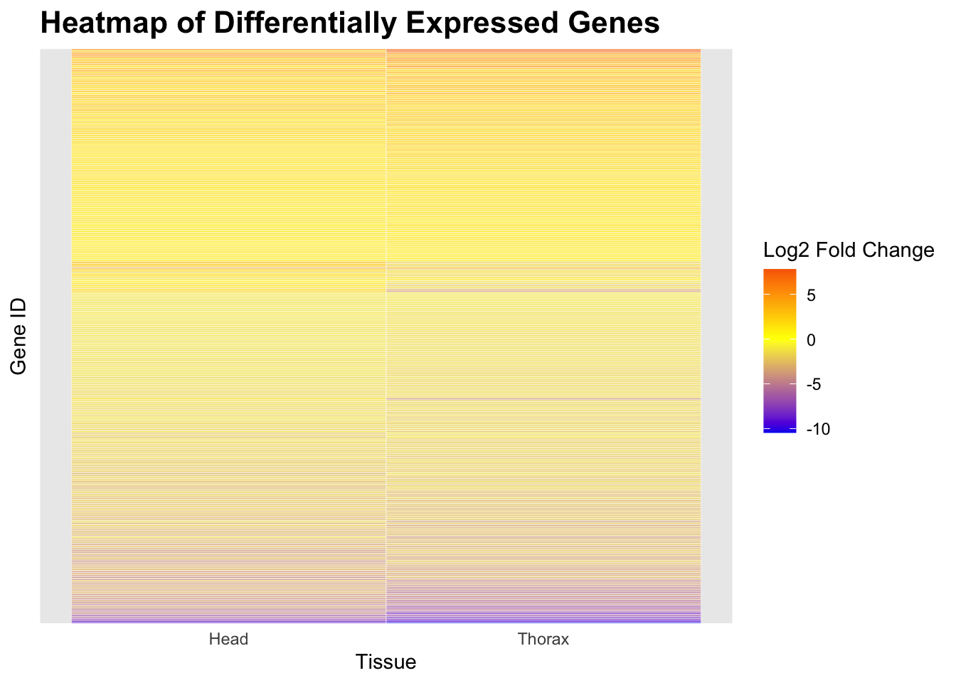
# Create heatmap plot
ggplot(heatmap_long, aes(x = Tissue, y = reorder(GeneID, Log2FoldChange), fill = Log2FoldChange)) +
    geom_tile(color = "white") +
    scale_fill_gradient2(low = "blue2", mid = "yellow", high = "red2", midpoint = 0, name = "Log2 Fold Change") +  # Make colors brighter
    labs(title = "Heatmap of Differentially Expressed Genes", x = "Tissue", y = "Gene ID") +
    theme_minimal() +
    theme(
        plot.title = element_text(size = 16, face = "bold"),
        axis.text.y = element_blank(),  # Remove row names
        axis.ticks.y = element_blank(),  # Remove y-axis ticks
        legend.position = "right"
    )

sessionInfo()

R version 4.4.1 (2024-06-14)
Platform: aarch64-apple-darwin20
Running under: macOS Sonoma 14.7

Matrix products: default
BLAS:   /Library/Frameworks/R.framework/Versions/4.4-arm64/Resources/lib/libRblas.0.dylib 
LAPACK: /Library/Frameworks/R.framework/Versions/4.4-arm64/Resources/lib/libRlapack.dylib;  LAPACK version 3.12.0

locale:
[1] en_US.UTF-8/en_US.UTF-8/en_US.UTF-8/C/en_US.UTF-8/en_US.UTF-8

time zone: America/Chicago
tzcode source: internal

attached base packages:
[1] grid      stats4    stats     graphics  grDevices utils     datasets 
[8] methods   base     

other attached packages:
 [1] reshape2_1.4.4       pheatmap_1.0.12      gridExtra_2.3       
 [4] VennDiagram_1.7.3    futile.logger_1.4.3  tibble_3.2.1        
 [7] tidyr_1.3.1          ggplot2_3.5.1        dplyr_1.1.4         
[10] topGO_2.56.0         SparseM_1.84-2       GO.db_3.19.1        
[13] AnnotationDbi_1.66.0 IRanges_2.38.1       S4Vectors_0.42.1    
[16] Biobase_2.64.0       graph_1.82.0         BiocGenerics_0.50.0 

loaded via a namespace (and not attached):
 [1] tidyselect_1.2.1        viridisLite_0.4.2       farver_2.1.2           
 [4] blob_1.2.4              Biostrings_2.72.1       fastmap_1.2.0          
 [7] promises_1.3.0          digest_0.6.37           lifecycle_1.0.4        
[10] KEGGREST_1.44.1         RSQLite_2.3.7           magrittr_2.0.3         
[13] compiler_4.4.1          rlang_1.1.4             sass_0.4.9             
[16] tools_4.4.1             utf8_1.2.4              yaml_2.3.10            
[19] knitr_1.48              lambda.r_1.2.4          labeling_0.4.3         
[22] bit_4.5.0               plyr_1.8.9              RColorBrewer_1.1-3     
[25] workflowr_1.7.1         withr_3.0.2             purrr_1.0.2            
[28] fansi_1.0.6             git2r_0.35.0            colorspace_2.1-1       
[31] scales_1.3.0            cli_3.6.3               rmarkdown_2.29         
[34] crayon_1.5.3            generics_0.1.3          rstudioapi_0.17.1      
[37] httr_1.4.7              DBI_1.2.3               cachem_1.1.0           
[40] stringr_1.5.1           zlibbioc_1.50.0         formatR_1.14           
[43] XVector_0.44.0          matrixStats_1.4.1       vctrs_0.6.5            
[46] jsonlite_1.8.9          bit64_4.5.2             jquerylib_0.1.4        
[49] glue_1.8.0              stringi_1.8.4           gtable_0.3.6           
[52] later_1.3.2             GenomeInfoDb_1.40.1     UCSC.utils_1.0.0       
[55] munsell_0.5.1           pillar_1.9.0            htmltools_0.5.8.1      
[58] GenomeInfoDbData_1.2.12 R6_2.5.1                rprojroot_2.0.4        
[61] evaluate_1.0.1          lattice_0.22-6          highr_0.11             
[64] futile.options_1.0.1    png_0.1-8               memoise_2.0.1          
[67] httpuv_1.6.15           bslib_0.8.0             Rcpp_1.0.13-1          
[70] whisker_0.4.1           xfun_0.49               fs_1.6.5               
[73] pkgconfig_2.0.3

Functional enrichment analysis

Maeva Techer

2024-11-06

1. Blast2Go file

Step 1: Load Genome (fasta + GFF)

Step 2: Run Blast

2. GO term enrichment

2.1. Load necessary libraries