Cross-species comparisons and DEGs overlap
Maeva Techer
2024-11-07
Last updated: 2024-11-07
Checks: 5 2
Knit directory:
locust-comparative-genomics/
This reproducible R Markdown analysis was created with workflowr (version 1.7.1). The Checks tab describes the reproducibility checks that were applied when the results were created. The Past versions tab lists the development history.
The R Markdown file has unstaged changes. To know which version of
the R Markdown file created these results, you’ll want to first commit
it to the Git repo. If you’re still working on the analysis, you can
ignore this warning. When you’re finished, you can run
wflow_publish to commit the R Markdown file and build the
HTML.
Great job! The global environment was empty. Objects defined in the global environment can affect the analysis in your R Markdown file in unknown ways. For reproduciblity it’s best to always run the code in an empty environment.
The command set.seed(20221025) was run prior to running
the code in the R Markdown file. Setting a seed ensures that any results
that rely on randomness, e.g. subsampling or permutations, are
reproducible.
Great job! Recording the operating system, R version, and package versions is critical for reproducibility.
Nice! There were no cached chunks for this analysis, so you can be confident that you successfully produced the results during this run.
Using absolute paths to the files within your workflowr project makes it difficult for you and others to run your code on a different machine. Change the absolute path(s) below to the suggested relative path(s) to make your code more reproducible.
| absolute | relative |
|---|---|
| /Users/maevatecher/Library/Mobile Documents/comappleCloudDocs/Documents/GitHub/locust-comparative-genomics/data | data |
Great! You are using Git for version control. Tracking code development and connecting the code version to the results is critical for reproducibility.
The results in this page were generated with repository version 9fb9741. See the Past versions tab to see a history of the changes made to the R Markdown and HTML files.
Note that you need to be careful to ensure that all relevant files for
the analysis have been committed to Git prior to generating the results
(you can use wflow_publish or
wflow_git_commit). workflowr only checks the R Markdown
file, but you know if there are other scripts or data files that it
depends on. Below is the status of the Git repository when the results
were generated:
Ignored files:
    Ignored:    .DS_Store
    Ignored:    .RData
    Ignored:    .Rhistory
    Ignored:    .Rproj.user/
    Ignored:    analysis/.DS_Store
    Ignored:    analysis/.Rhistory
    Ignored:    data/.DS_Store
    Ignored:    data/.Rhistory
    Ignored:    data/OLD/.DS_Store
    Ignored:    data/OLD/DEseq2_SCUBE_SCUBE_THORAX_STARnew_features/.DS_Store
    Ignored:    data/OLD/DEseq2_SGREG_SGREG_HEAD_STARnew_features/.DS_Store
    Ignored:    data/OLD/DEseq2_SGREG_SGREG_THORAX_STARnew_features/.DS_Store
    Ignored:    data/OLD/americana/.DS_Store
    Ignored:    data/OLD/americana/deg_counts/.DS_Store
    Ignored:    data/OLD/americana/deg_counts/STAR_newparams/.DS_Store
    Ignored:    data/OLD/cubense/deg_counts/STAR/cubense/featurecounts/
    Ignored:    data/OLD/cubense/deg_counts/STAR/gregaria/
    Ignored:    data/OLD/gregaria/.DS_Store
    Ignored:    data/OLD/gregaria/deg_counts/.DS_Store
    Ignored:    data/OLD/gregaria/deg_counts/STAR/.DS_Store
    Ignored:    data/OLD/gregaria/deg_counts/STAR/gregaria/.DS_Store
    Ignored:    data/OLD/gregaria/deg_counts/STAR_newparams/.DS_Store
    Ignored:    data/OLD/piceifrons/.DS_Store
    Ignored:    data/list/.DS_Store
    Ignored:    figures/
    Ignored:    tables/

Untracked files:
    Untracked:  data/03-americana-DESeq2-togregaria/
    Untracked:  data/03-cancellata-DESeq2-togregaria/
    Untracked:  data/03-cubense-DESeq2-togregaria/
    Untracked:  data/03-gregaria-DESeq2-togregaria/
    Untracked:  data/03-nitens-DESeq2-togregaria/
    Untracked:  data/03-piceifrons-DESeq2-togregaria/
    Untracked:  data/DEG-results/
    Untracked:  data/list/GO_Annotations/
    Untracked:  data/list/allspecies_geneid.csv
    Untracked:  data/list/allspecies_protein2geneid.tsv
    Untracked:  data/orthofinder/

Unstaged changes:
    Modified:   analysis/1_seq-data.Rmd
    Modified:   analysis/2_orthologs-prediction.Rmd
    Modified:   analysis/3_deseq2-results.Rmd
    Modified:   analysis/3_go-enrichment.Rmd
    Modified:   analysis/3_overlap-venn.Rmd
    Modified:   analysis/3_seq-data-qc.Rmd
    Modified:   analysis/_site.yml
    Deleted:    data/list/tx2gene.americana.csv
Note that any generated files, e.g. HTML, png, CSS, etc., are not included in this status report because it is ok for generated content to have uncommitted changes.
These are the previous versions of the repository in which changes were
made to the R Markdown (analysis/3_overlap-venn.Rmd) and
HTML (docs/3_overlap-venn.html) files. If you’ve configured
a remote Git repository (see ?wflow_git_remote), click on
the hyperlinks in the table below to view the files as they were in that
past version.
| File | Version | Author | Date | Message |
|---|---|---|---|---|
| html | ba35b82 | Maeva A. TECHER | 2024-06-19 | Build site. |
| html | 45d0b6b | Maeva A. TECHER | 2024-05-15 | Build site. |
| Rmd | 5dff93d | Maeva A. TECHER | 2024-05-15 | wflow_publish("analysis/3_overlap-venn.Rmd") |
We start by loading all the required R packages.
#(install first from CRAN or Bioconductor)
library(knitr)
library(dplyr)
library(ggplot2)
library(plotly)
library(htmlwidgets)  # For saving interactive plots
library(ggVennDiagram)
library(pheatmap)
library(tidyr)
library(RColorBrewer)
library(viridis)
library(kableExtra)
library(tibble)

# Path for all species
workDir <- "/Users/maevatecher/Library/Mobile Documents/com~apple~CloudDocs/Documents/GitHub/locust-comparative-genomics/data"
allspecies_path <- file.path(workDir, "/list/allspecies_geneid.csv")
allspecies_df <- read.table(allspecies_path, sep = ",", header = TRUE, quote = "", fill = TRUE, stringsAsFactors = FALSE)
species_list <- c("gregaria", "piceifrons", "cancellata", "americana", "cubense", "nitens")
Here our objective is to compare the abundance, composition and
overlap of the DEGs found in the head and thorax tissues of each species
between the isolated and crowded last instar females. We found that the
differential genes expressed detected by DESeq2 varied
across species and tissues but we need some perspective: Are locusts
up-regulated and down-regulated the same genes? In the later section GO
enrichment, we will investigate what are the functions of these genes as
we will see that each species seems to show different gene expression
profiles in response to density changes.
STRATEGY 1: One genome S. gregaria
1. DEGs comparison among species
We summarized the number of genes differential expressed between density for each species and each tissues.
# Initialize an empty data frame to store results
summary_table_head <- data.frame(Species = character(),
                            Head_Upregulated = integer(),
                            Head_Upregulated_Strict = integer(),
                            Head_Downregulated = integer(),
                            Head_Downregulated_Strict = integer(),
                            stringsAsFactors = FALSE)

summary_table_thorax <- data.frame(Species = character(),
                            Thorax_Upregulated = integer(),
                            Thorax_Upregulated_Strict = integer(),
                            Thorax_Downregulated = integer(),
                            Thorax_Downregulated_Strict = integer(),
                            stringsAsFactors = FALSE)


# Loop through each species to process their data
for (species in species_list) {
    # Read the DESeq2 results and sigresults files
    head_sigresults_file <- file.path(workDir, "DEG-results", paste0("DESeq2_sigresults_Head_togregaria_", species, ".csv"))
    thorax_sigresults_file <- file.path(workDir, "DEG-results", paste0("DESeq2_sigresults_Thorax_togregaria_", species, ".csv"))

    head_sigresults <- read.csv(head_sigresults_file, stringsAsFactors = FALSE)
    thorax_sigresults <- read.csv(thorax_sigresults_file, stringsAsFactors = FALSE)

    # Count upregulated and downregulated genes for head
    head_upregulated <- nrow(head_sigresults %>% filter(log2FoldChange > 0))
    head_downregulated <- nrow(head_sigresults %>% filter(log2FoldChange < -0))
    head_upregulated_strict <- nrow(head_sigresults %>% filter(log2FoldChange > 1))
    head_downregulated_strict <- nrow(head_sigresults %>% filter(log2FoldChange < -1))

    # Count upregulated and downregulated genes for thorax
    thorax_upregulated <- nrow(thorax_sigresults %>% filter(log2FoldChange > 0))
    thorax_downregulated <- nrow(thorax_sigresults %>% filter(log2FoldChange < -0))
    thorax_upregulated_strict <- nrow(thorax_sigresults %>% filter(log2FoldChange > 1))
    thorax_downregulated_strict <- nrow(thorax_sigresults %>% filter(log2FoldChange < -1))

    # Add to the summary table
    summary_table_head <- rbind(summary_table_head, data.frame("Species" = species,
                                                      "Head_Upregulated" = head_upregulated,
                                                      "Head_Downregulated" = head_downregulated,
                                                      "Head_Upregulated_Strict" = head_upregulated_strict,
                                                      "Head_Downregulated_Strict" = head_downregulated_strict,
                                                      stringsAsFactors = FALSE))

    summary_table_thorax <- rbind(summary_table_thorax, data.frame("Species" = species,
                                                      "Thorax_Upregulated" = thorax_upregulated,
                                                      "Thorax_Downregulated" = thorax_downregulated,
                                                      "Thorax_Upregulated_Strict" = thorax_upregulated_strict,
                                                      "Thorax_Downregulated_Strict" = thorax_downregulated_strict,
                                                      stringsAsFactors = FALSE))
}

# Print the summary table in a markdown-friendly format
knitr::kable(summary_table_head, format = "markdown", caption = "Summary of differentially expressed genes in head per species")| Species | Head_Upregulated | Head_Downregulated | Head_Upregulated_Strict | Head_Downregulated_Strict |
|---|---|---|---|---|
| gregaria | 2709 | 2988 | 814 | 662 |
| piceifrons | 375 | 375 | 194 | 191 |
| cancellata | 689 | 756 | 301 | 386 |
| americana | 703 | 487 | 311 | 256 |
| cubense | 30 | 31 | 30 | 31 |
| nitens | 189 | 259 | 104 | 207 |
# Convert the summary table to a long format for easier plotting
summary_long_head <- summary_table_head %>%
  select(Species, Head_Upregulated_Strict, Head_Downregulated_Strict) %>%
  pivot_longer(cols = -Species,
               names_to = c(".value", "Tissue"),
               names_sep = "_")


# Adjust the values for downregulated genes to be negative
summary_long_head <- summary_long_head %>%
  mutate(Head = ifelse(Tissue == "Downregulated", -Head, Head))

summary_long_head$Species <- factor(summary_long_head$Species, levels = species_list)
# Now create a barplot for head
ggplot(summary_long_head, aes(x = Species, y = Head, fill = Tissue)) +
  geom_bar(stat = "identity", position = "dodge") +
  labs(title = "Upregulated and Downregulated Genes in Head Tissues (lfc > 1)",
       x = "Species",
       y = "Number of Genes") +
  scale_fill_manual(values = c("Upregulated" = "red2", "Downregulated" = "blue")) +
  scale_y_continuous(labels = function(x) ifelse(x < 0, -x, x), limits = c(-1200, 850)) + # Set fixed y-axis limits
  theme_minimal(base_size = 12) + # Increase base font size for better readability
  theme(legend.position = "top",
        plot.title = element_text(hjust = 0.5, size = 14, face = "bold"),
        axis.title.x = element_text(size = 14, face = "bold"),
        axis.title.y = element_text(size = 14, face = "bold"),
        axis.text.x = element_text(size = 12, angle = 45, hjust = 1),  # Adjust text size and angle for x-axis
        axis.text.y = element_text(size = 12),
        panel.grid.major.y = element_line(color = "grey90", linetype = "dashed"),
        panel.grid.minor = element_blank())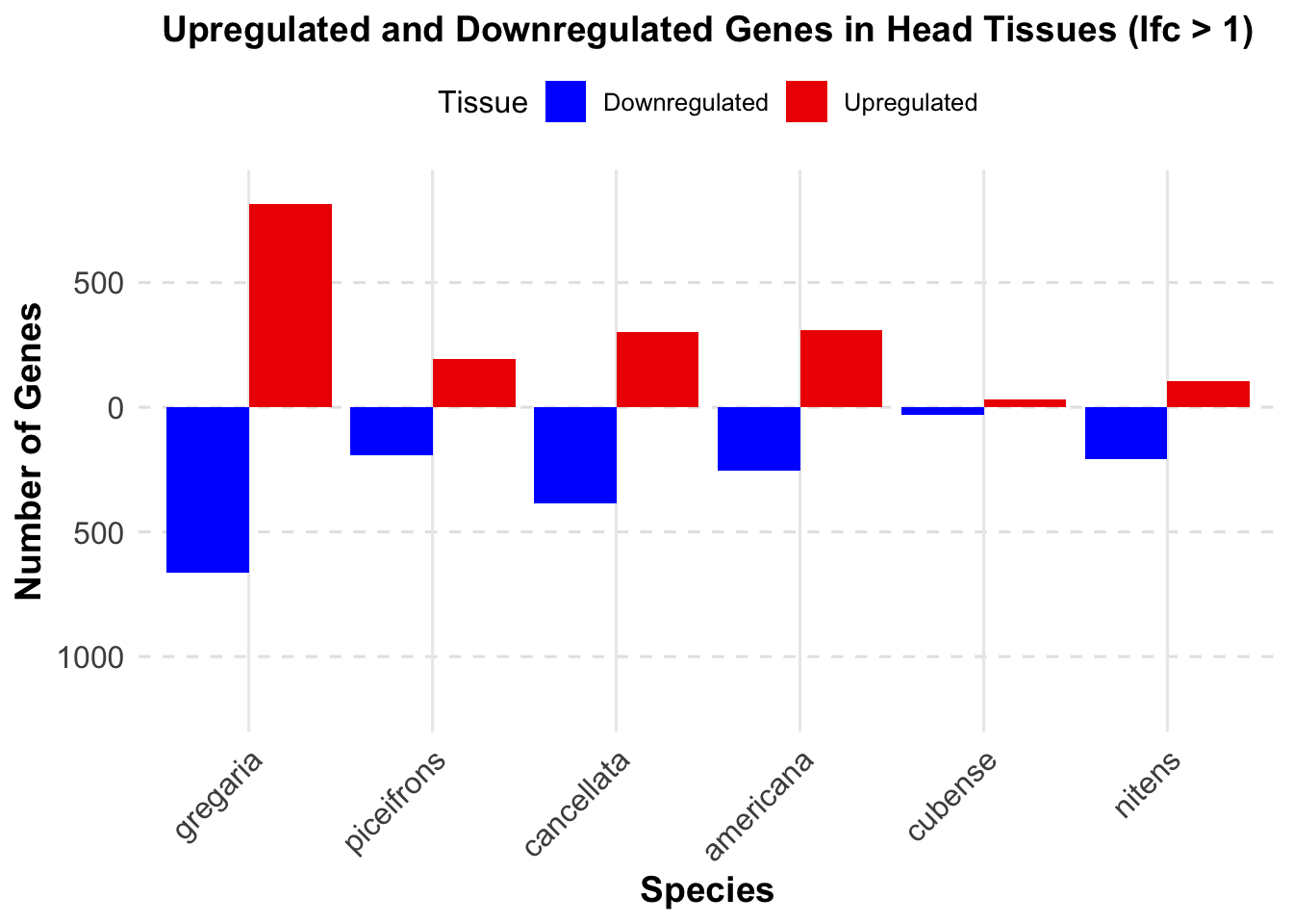
knitr::kable(summary_table_thorax, format = "markdown", caption = "Summary of differentially expressed genes in thorax per species")| Species | Thorax_Upregulated | Thorax_Downregulated | Thorax_Upregulated_Strict | Thorax_Downregulated_Strict |
|---|---|---|---|---|
| gregaria | 2751 | 2691 | 622 | 1174 |
| piceifrons | 1517 | 1200 | 549 | 221 |
| cancellata | 686 | 648 | 289 | 303 |
| americana | 398 | 699 | 149 | 339 |
| cubense | 104 | 218 | 64 | 154 |
| nitens | 0 | 0 | 0 | 0 |
# Convert the summary table to a long format for easier plotting
summary_long_thorax <- summary_table_thorax %>%
  select(Species, Thorax_Upregulated_Strict, Thorax_Downregulated_Strict) %>%
  pivot_longer(cols = -Species,
               names_to = c(".value", "Tissue"),
               names_sep = "_")

# Adjust the values for downregulated genes to be negative
summary_long_thorax <- summary_long_thorax %>%
  mutate(Thorax = ifelse(Tissue == "Downregulated", -Thorax, Thorax))

summary_long_thorax$Species <- factor(summary_long_thorax$Species, levels = species_list)
# Now create a barplot for head
ggplot(summary_long_thorax, aes(x = Species, y = Thorax, fill = Tissue)) +
  geom_bar(stat = "identity", position = "dodge") +
  labs(title = "Upregulated and Downregulated Genes in Thorax Tissues (lfc > 1)",
       x = "Species",
       y = "Number of Genes") +
  scale_fill_manual(values = c("Upregulated" = "red2", "Downregulated" = "blue")) +
  scale_y_continuous(labels = function(x) ifelse(x < 0, -x, x), limits = c(-1200, 850)) + # Set fixed y-axis limits
  theme_minimal(base_size = 12) + # Increase base font size for better readability
  theme(legend.position = "top",
        plot.title = element_text(hjust = 0.5, size = 14, face = "bold"),
        axis.title.x = element_text(size = 14, face = "bold"),
        axis.title.y = element_text(size = 14, face = "bold"),
        axis.text.x = element_text(size = 12, angle = 45, hjust = 1),  # Adjust text size and angle for x-axis
        axis.text.y = element_text(size = 12),
        panel.grid.major.y = element_line(color = "grey90", linetype = "dashed"),
        panel.grid.minor = element_blank())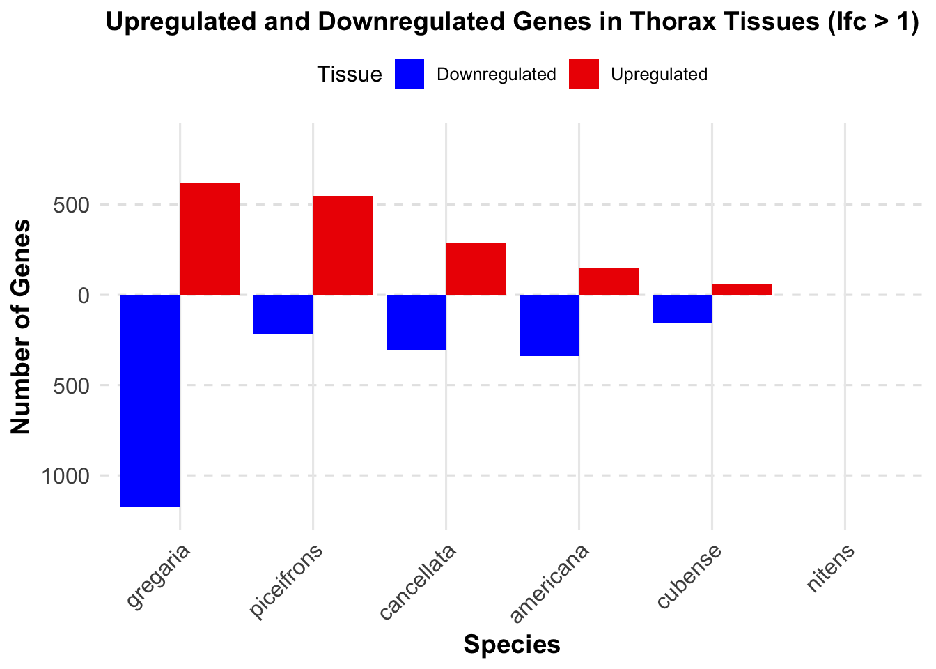
2. Overlap DEGs between tissues
species_list5 <- c("gregaria", "piceifrons", "cancellata", "americana", "cubense", "nitens")
# Loop through each species to process their data
for (species in species_list5) {
# Load DESeq2 results for head and thorax
head_file <- file.path(workDir, "DEG-results", paste0("DESeq2_results_Head_togregaria_", species, ".csv"))
thorax_file <- file.path(workDir, "DEG-results", paste0("DESeq2_results_Thorax_togregaria_", species, ".csv"))
head_data <- read.csv(head_file, stringsAsFactors = FALSE)
thorax_data <- read.csv(thorax_file, stringsAsFactors = FALSE)
# Check if data is empty and handle accordingly
if (nrow(head_data) == 0 || nrow(thorax_data) == 0) {
message(paste("No data for species:", species))
next # Skip to the next species if there's no data
}
# Filter significant DEGs for both head and thorax
head_sig_genes <- head_data %>%
filter(padj < 0.05 & abs(log2FoldChange) > 1) %>%
select(GeneID = X, log2FoldChange, padj)
thorax_sig_genes <- thorax_data %>%
filter(padj < 0.05 & abs(log2FoldChange) > 1) %>%
select(GeneID = X, log2FoldChange, padj)
# Find overlapping genes based on GeneID
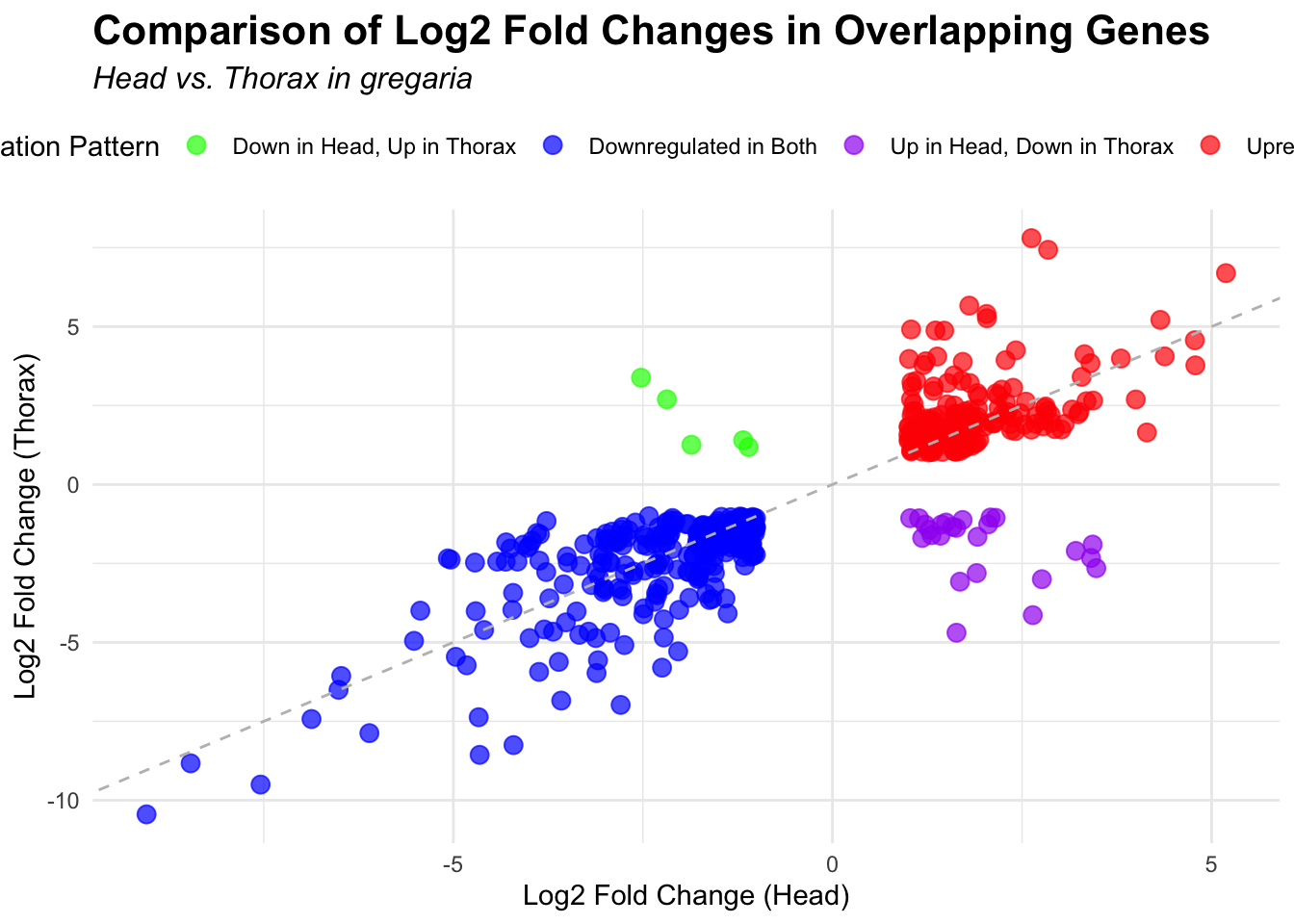
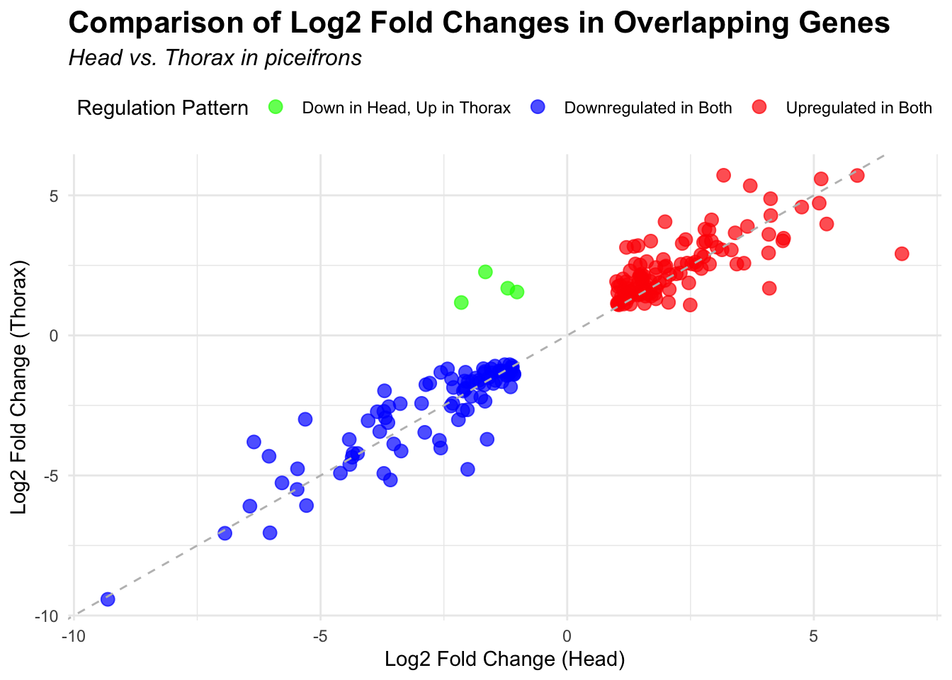
overlapping_genes <- inner_join(head_sig_genes, thorax_sig_genes, by = "GeneID", suffix = c("_head", "_thorax"))
# Save the overlapping genes to a CSV file
output_file <- file.path(workDir, "DEG-results", paste0("overlapping_genes_head_thorax_", species, ".csv"))
write.csv(overlapping_genes, output_file, row.names = FALSE)
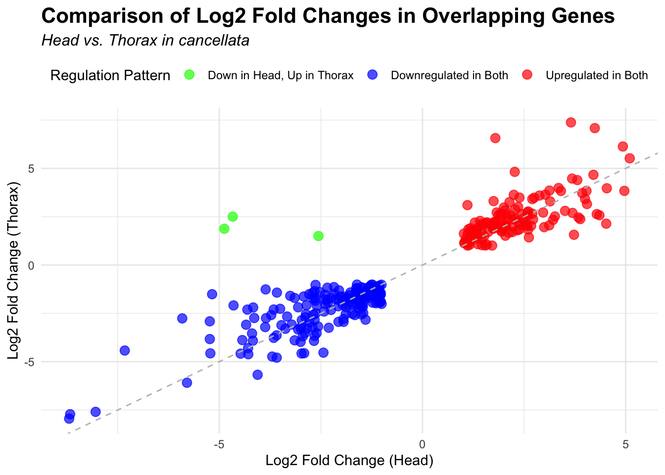
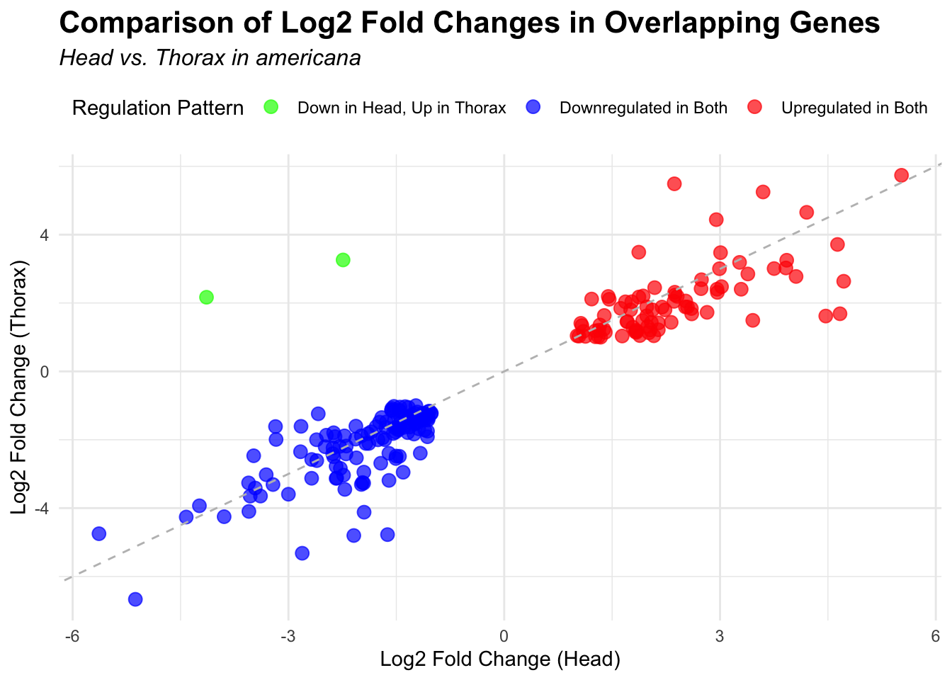
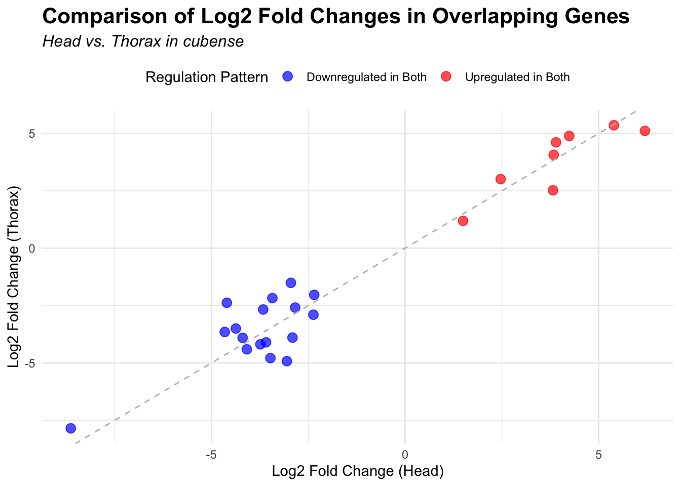
# Plot overlapping genes with scatter plot
p <- ggplot(overlapping_genes, aes(x = log2FoldChange_head, y = log2FoldChange_thorax)) +
geom_point(aes(color = case_when(
log2FoldChange_head > 0 & log2FoldChange_thorax > 0 ~ "Upregulated in Both",
log2FoldChange_head < 0 & log2FoldChange_thorax < 0 ~ "Downregulated in Both",
log2FoldChange_head > 0 & log2FoldChange_thorax < 0 ~ "Up in Head, Down in Thorax",
log2FoldChange_head < 0 & log2FoldChange_thorax > 0 ~ "Down in Head, Up in Thorax"
)), size = 3, alpha = 0.7) +
geom_abline(slope = 1, intercept = 0, linetype = "dashed", color = "gray") +
labs(
x = "Log2 Fold Change (Head)",
y = "Log2 Fold Change (Thorax)",
color = "Regulation Pattern",
title = "Comparison of Log2 Fold Changes in Overlapping Genes",
subtitle = paste("Head vs. Thorax in", species)
) +
theme_minimal() +
theme(
plot.title = element_text(size = 16, face = "bold"),
plot.subtitle = element_text(size = 12, face = "italic"),
legend.position = "top"
) +
scale_color_manual(values = c(
"Upregulated in Both" = "red",
"Downregulated in Both" = "blue",
"Up in Head, Down in Thorax" = "purple",
"Down in Head, Up in Thorax" = "green"
))
# Save the static plot
ggsave(filename = file.path(workDir, "DEG-results", paste0("scatter_plot_overlapping_genes_", species, ".png")), plot = p)
print(p)
# Convert to interactive Plotly plot
interactive_plot <- ggplotly(p) %>%
layout(title = paste("Scatter Plot of Overlapping Genes:", species), hoverlabel = list(bgcolor = "white"))
}
3. Overlap DEGs among species
COMBINED
# Initialize an empty list to store heatmap data for each species
heatmap_list <- list()
# Loop through each species to process their data
for (species in species_list) {
# Load DESeq2 results for head and thorax
head_file <- file.path(workDir, "DEG-results", paste0("DESeq2_sigresults_Head_togregaria_", species, ".csv"))
thorax_file <- file.path(workDir, "DEG-results", paste0("DESeq2_sigresults_Thorax_togregaria_", species, ".csv"))
# Load the data
head_data <- read.csv(head_file, stringsAsFactors = FALSE)
thorax_data <- read.csv(thorax_file, stringsAsFactors = FALSE)
# Check if data is empty and handle accordingly
if (nrow(head_data) == 0 || nrow(thorax_data) == 0) {
message(paste("No data for species:", species))
next # Skip to the next species if there's no data
}
# Filter for significant DEGs and select top 100 upregulated and downregulated genes for each tissue
head_up <- head_data %>%
filter(padj < 0.05 & log2FoldChange > 1) %>%
arrange(desc(log2FoldChange)) %>%
slice(1:500)
head_down <- head_data %>%
filter(padj < 0.05 & log2FoldChange < -1) %>%
arrange(log2FoldChange) %>%
slice(1:500)
thorax_up <- thorax_data %>%
filter(padj < 0.05 & log2FoldChange > 1) %>%
arrange(desc(log2FoldChange)) %>%
slice(1:500)
thorax_down <- thorax_data %>%
filter(padj < 0.05 & log2FoldChange < -1) %>%
arrange(log2FoldChange) %>%
slice(1:500)
# Combine data and prepare for heatmap, adding the species column
heatmap_data <- bind_rows(
head_up %>% mutate(Tissue = "Head", Regulation = "Upregulated", Species = species),
head_down %>% mutate(Tissue = "Head", Regulation = "Downregulated", Species = species),
thorax_up %>% mutate(Tissue = "Thorax", Regulation = "Upregulated", Species = species),
thorax_down %>% mutate(Tissue = "Thorax", Regulation = "Downregulated", Species = species)
) %>%
select(GeneID, log2FoldChange, Tissue, Regulation, Species)
# Append the heatmap data to the list
heatmap_list[[species]] <- heatmap_data
}
# Combine all species data into a single dataframe for heatmap matrix preparation
final_heatmap_data <- bind_rows(heatmap_list)
# Check if final_heatmap_data is empty before proceeding
if (nrow(final_heatmap_data) == 0) {
stop("No valid data available for heatmap generation.")
}
# Create heatmap matrix
heatmap_matrix <- final_heatmap_data %>%
group_by(GeneID, Species) %>%
summarize(
Head_Combined = sum(log2FoldChange[Tissue == "Head"], na.rm = TRUE),
Thorax_Combined = sum(log2FoldChange[Tissue == "Thorax"], na.rm = TRUE),
.groups = 'drop'
) %>%
pivot_longer(cols = c("Head_Combined", "Thorax_Combined"),
names_to = c("Tissue", ".value"),
names_sep = "_") %>%
# Combine the Head and Thorax values for each GeneID while keeping Species
group_by(GeneID, Species) %>%
summarize(
Head = sum(ifelse(Tissue == "Head", Combined, 0), na.rm = TRUE),
Thorax = sum(ifelse(Tissue == "Thorax", Combined, 0), na.rm = TRUE),
.groups = 'drop'
) %>%
pivot_wider(names_from = Species,
values_from = c(Head, Thorax),
values_fill = list(Head = 0, Thorax = 0)) %>%
column_to_rownames("GeneID") %>%
as.matrix()
color_palette <- c("cyan", "cyan2", "cyan3", "black", "orange3", "orange2", "orange")
color_palette2 <- c("blue3", "blue2", "blue1", "white", "red", "red2", "red3")
# Create heatmap
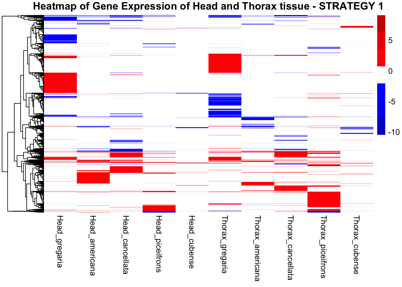
pheatmap(
heatmap_matrix,
color = color_palette2,
cluster_rows = TRUE, # Set to TRUE to cluster genes
cluster_cols = FALSE, # Set to TRUE to cluster samples
show_rownames = FALSE, # Show gene IDs
show_colnames = TRUE, # Show tissue and species names
fontsize_row = 6, # Adjust font size for rows if necessary
fontsize_col = 10, # Adjust font size for columns if necessary
main = "Heatmap of Gene Expression of Head and Thorax tissue - STRATEGY 1"
)
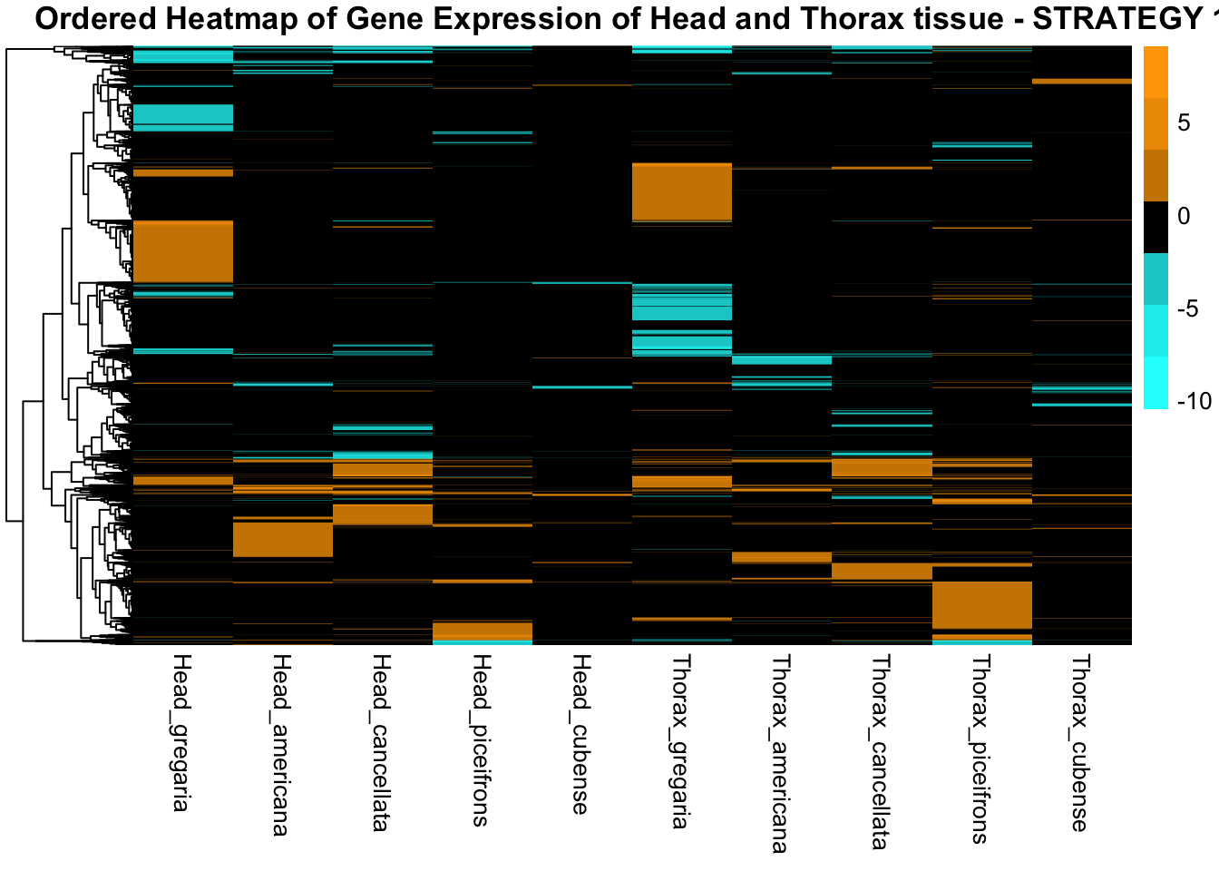
pheatmap(
  heatmap_matrix,
  color = color_palette,
  cluster_rows = TRUE,  # Set to TRUE to cluster genes
  cluster_cols = FALSE,  # Set to FALSE to prevent clustering on columns
  show_rownames = FALSE,  # Hide gene IDs
  show_colnames = TRUE,   # Show tissue and species names
  fontsize_row = 6,       # Adjust font size for rows if necessary
  fontsize_col = 10,      # Adjust font size for columns if necessary
  main = "Ordered Heatmap of Gene Expression of Head and Thorax tissue - STRATEGY 1"
)
HEAD ONLY
# Initialize an empty list to store heatmap data for each species
heatmap_list <- list()
# Loop through each species to process their data
for (species in species_list) {
# Load DESeq2 results for head and thorax
head_file <- file.path(workDir, "DEG-results", paste0("DESeq2_sigresults_Head_togregaria_", species, ".csv"))
# Load the data
head_data <- read.csv(head_file, stringsAsFactors = FALSE)
# Check if data is empty and handle accordingly
if (nrow(head_data) == 0) {
message(paste("No data for species:", species))
next # Skip to the next species if there's no data
}
# Filter for significant DEGs and select top 100 upregulated and downregulated genes for each tissue
head_up <- head_data %>%
filter(padj < 0.05 & log2FoldChange > 1) %>%
arrange(desc(log2FoldChange)) %>%
slice(1:500)
head_down <- head_data %>%
filter(padj < 0.05 & log2FoldChange < -1) %>%
arrange(log2FoldChange) %>%
slice(1:500)
# Combine data and prepare for heatmap, adding the species column
heatmap_data <- bind_rows(
head_up %>% mutate(Tissue = "Head", Regulation = "Upregulated", Species = species),
head_down %>% mutate(Tissue = "Head", Regulation = "Downregulated", Species = species)
) %>%
select(GeneID, log2FoldChange, Tissue, Regulation, Species)
# Append the heatmap data to the list
heatmap_list[[species]] <- heatmap_data
}
# Combine all species data into a single dataframe for heatmap matrix preparation
final_heatmap_data <- bind_rows(heatmap_list)
# Check if final_heatmap_data is empty before proceeding
if (nrow(final_heatmap_data) == 0) {
stop("No valid data available for heatmap generation.")
}
# Create heatmap matrix
heatmap_matrix <- final_heatmap_data %>%
group_by(GeneID, Species) %>%
summarize(
Head_Combined = sum(log2FoldChange[Tissue == "Head"], na.rm = TRUE),
.groups = 'drop'
) %>%
pivot_longer(cols = c("Head_Combined"),
names_to = c("Tissue", ".value"),
names_sep = "_") %>%
# Combine the Head and Thorax values for each GeneID while keeping Species
group_by(GeneID, Species) %>%
summarize(
Head = sum(ifelse(Tissue == "Head", Combined, 0), na.rm = TRUE),
.groups = 'drop'
) %>%
pivot_wider(names_from = Species,
values_from = c(Head),
values_fill = list(Head = 0)) %>%
column_to_rownames("GeneID") %>%
as.matrix()
color_palette <- c("cyan", "cyan2", "cyan3", "black", "orange3", "orange2", "orange")
color_palette2 <- c("blue3", "blue2", "blue1", "white", "red", "red2", "red3")
# Create heatmap
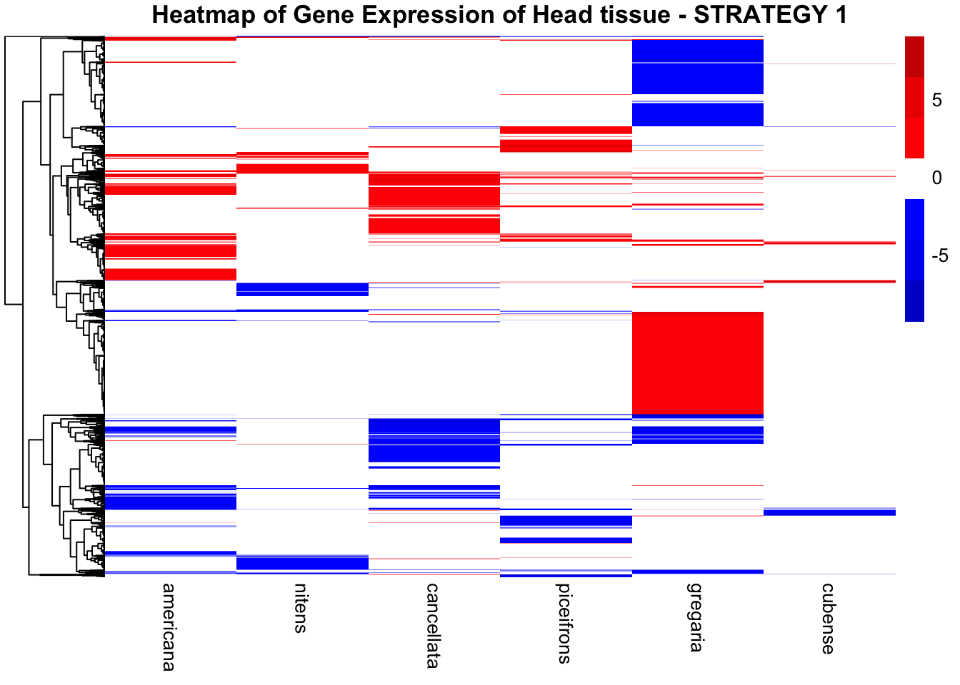
pheatmap(
heatmap_matrix,
color = color_palette2,
cluster_rows = TRUE, # Set to TRUE to cluster genes
cluster_cols = FALSE, # Set to TRUE to cluster samples
show_rownames = FALSE, # Show gene IDs
show_colnames = TRUE, # Show tissue and species names
fontsize_row = 6, # Adjust font size for rows if necessary
fontsize_col = 10, # Adjust font size for columns if necessary
main = "Heatmap of Gene Expression of Head tissue - STRATEGY 1"
)
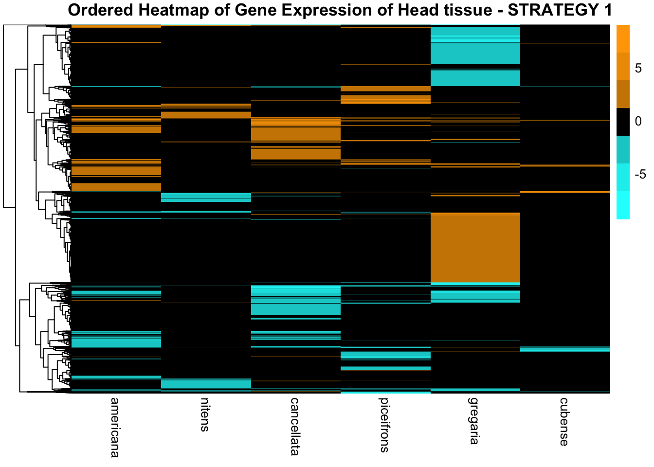
pheatmap(
  heatmap_matrix,
  color = color_palette,
  cluster_rows = TRUE,  # Set to TRUE to cluster genes
  cluster_cols = FALSE,  # Set to FALSE to prevent clustering on columns
  show_rownames = FALSE,  # Hide gene IDs
  show_colnames = TRUE,   # Show tissue and species names
  fontsize_row = 6,       # Adjust font size for rows if necessary
  fontsize_col = 10,      # Adjust font size for columns if necessary
  main = "Ordered Heatmap of Gene Expression of Head tissue - STRATEGY 1"
)
THORAX ONLY
# Initialize an empty list to store heatmap data for each species
heatmap_list <- list()
# Loop through each species to process their data
for (species in species_list) {
# Load DESeq2 results for head and thorax
thorax_file <- file.path(workDir, "DEG-results", paste0("DESeq2_sigresults_Thorax_togregaria_", species, ".csv"))
# Load the data
thorax_data <- read.csv(thorax_file, stringsAsFactors = FALSE)
# Check if data is empty and handle accordingly
if (nrow(thorax_data) == 0) {
message(paste("No data for species:", species))
next # Skip to the next species if there's no data
}
# Filter for significant DEGs and select top 100 upregulated and downregulated genes for each tissue
thorax_up <- thorax_data %>%
filter(padj < 0.05 & log2FoldChange > 1) %>%
arrange(desc(log2FoldChange)) %>%
slice(1:500)
thorax_down <- thorax_data %>%
filter(padj < 0.05 & log2FoldChange < -1) %>%
arrange(log2FoldChange) %>%
slice(1:500)
# Combine data and prepare for heatmap, adding the species column
heatmap_data <- bind_rows(
thorax_up %>% mutate(Tissue = "Thorax", Regulation = "Upregulated", Species = species),
thorax_down %>% mutate(Tissue = "Thorax", Regulation = "Downregulated", Species = species)
) %>%
select(GeneID, log2FoldChange, Tissue, Regulation, Species)
# Append the heatmap data to the list
heatmap_list[[species]] <- heatmap_data
}
# Combine all species data into a single dataframe for heatmap matrix preparation
final_heatmap_data <- bind_rows(heatmap_list)
# Check if final_heatmap_data is empty before proceeding
if (nrow(final_heatmap_data) == 0) {
stop("No valid data available for heatmap generation.")
}
# Create heatmap matrix
heatmap_matrix <- final_heatmap_data %>%
group_by(GeneID, Species) %>%
summarize(
Thorax_Combined = sum(log2FoldChange[Tissue == "Thorax"], na.rm = TRUE),
.groups = 'drop'
) %>%
pivot_longer(cols = c( "Thorax_Combined"),
names_to = c("Tissue", ".value"),
names_sep = "_") %>%
# Combine the Head and Thorax values for each GeneID while keeping Species
group_by(GeneID, Species) %>%
summarize(
Thorax = sum(ifelse(Tissue == "Thorax", Combined, 0), na.rm = TRUE),
.groups = 'drop'
) %>%
pivot_wider(names_from = Species,
values_from = c(Thorax),
values_fill = list(Thorax = 0)) %>%
column_to_rownames("GeneID") %>%
as.matrix()
color_palette <- c("cyan", "black", "orange")
color_palette2 <- c("blue3", "white", "red3")
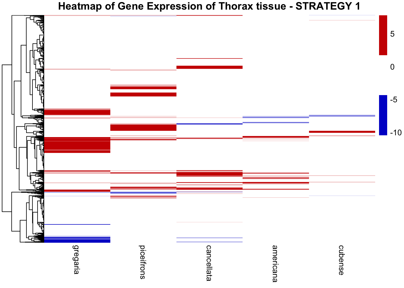
# Create heatmap
pheatmap(
heatmap_matrix,
color = color_palette2,
cluster_rows = TRUE, # Set to TRUE to cluster genes
cluster_cols = FALSE, # Set to TRUE to cluster samples
show_rownames = FALSE, # Show gene IDs
show_colnames = TRUE, # Show tissue and species names
fontsize_row = 6, # Adjust font size for rows if necessary
fontsize_col = 10, # Adjust font size for columns if necessary
main = "Heatmap of Gene Expression of Thorax tissue - STRATEGY 1"
)
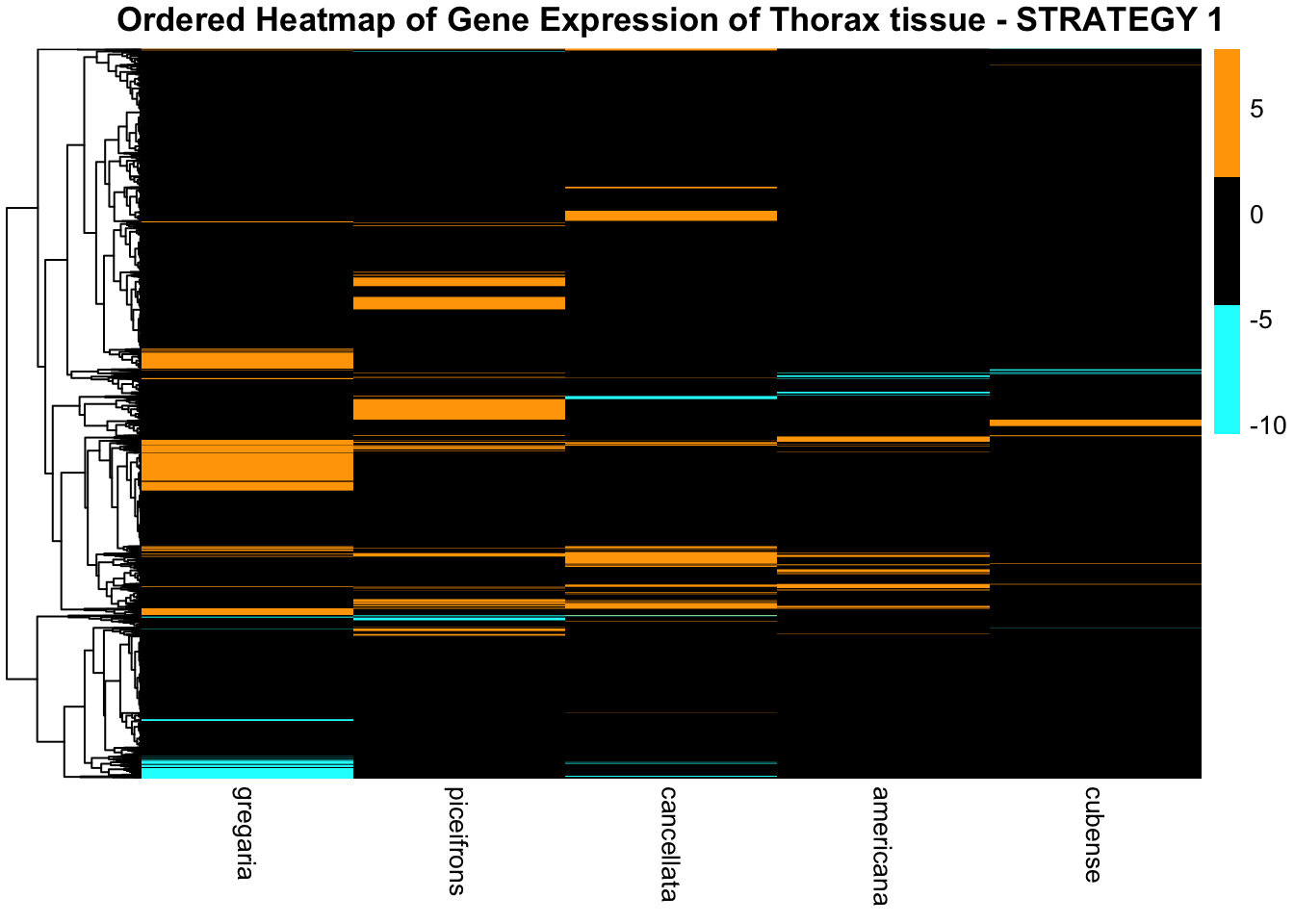
pheatmap(
  heatmap_matrix,
  color = color_palette,
  cluster_rows = TRUE,  # Set to TRUE to cluster genes
  cluster_cols = FALSE,  # Set to FALSE to prevent clustering on columns
  show_rownames = FALSE,  # Hide gene IDs
  show_colnames = TRUE,   # Show tissue and species names
  fontsize_row = 6,       # Adjust font size for rows if necessary
  fontsize_col = 10,      # Adjust font size for columns if necessary
  main = "Ordered Heatmap of Gene Expression of Thorax tissue - STRATEGY 1"
)
STRATEGY 2: Own RefSeq genome
sessionInfo()R version 4.4.1 (2024-06-14)
Platform: aarch64-apple-darwin20
Running under: macOS Sonoma 14.7
Matrix products: default
BLAS: /Library/Frameworks/R.framework/Versions/4.4-arm64/Resources/lib/libRblas.0.dylib
LAPACK: /Library/Frameworks/R.framework/Versions/4.4-arm64/Resources/lib/libRlapack.dylib; LAPACK version 3.12.0
locale:
[1] en_US.UTF-8/en_US.UTF-8/en_US.UTF-8/C/en_US.UTF-8/en_US.UTF-8
time zone: America/Chicago
tzcode source: internal
attached base packages:
[1] stats graphics grDevices utils datasets methods base
other attached packages:
[1] tibble_3.2.1 kableExtra_1.4.0 viridis_0.6.5
[4] viridisLite_0.4.2 RColorBrewer_1.1-3 tidyr_1.3.1
[7] pheatmap_1.0.12 ggVennDiagram_1.5.3 htmlwidgets_1.6.4
[10] plotly_4.10.4 ggplot2_3.5.1 dplyr_1.1.4
[13] knitr_1.48
loaded via a namespace (and not attached):
[1] sass_0.4.9 utf8_1.2.4 generics_0.1.3 xml2_1.3.6
[5] stringi_1.8.4 digest_0.6.37 magrittr_2.0.3 evaluate_1.0.1
[9] grid_4.4.1 fastmap_1.2.0 rprojroot_2.0.4 workflowr_1.7.1
[13] jsonlite_1.8.9 whisker_0.4.1 gridExtra_2.3 promises_1.3.0
[17] httr_1.4.7 purrr_1.0.2 fansi_1.0.6 crosstalk_1.2.1
[21] scales_1.3.0 textshaping_0.4.0 lazyeval_0.2.2 jquerylib_0.1.4
[25] cli_3.6.3 rlang_1.1.4 munsell_0.5.1 withr_3.0.2
[29] cachem_1.1.0 yaml_2.3.10 tools_4.4.1 colorspace_2.1-1
[33] httpuv_1.6.15 vctrs_0.6.5 R6_2.5.1 lifecycle_1.0.4
[37] git2r_0.35.0 stringr_1.5.1 fs_1.6.5 ragg_1.3.3
[41] pkgconfig_2.0.3 pillar_1.9.0 bslib_0.8.0 later_1.3.2
[45] gtable_0.3.6 glue_1.8.0 data.table_1.16.2 Rcpp_1.0.13-1
[49] systemfonts_1.1.0 xfun_0.49 tidyselect_1.2.1 highr_0.11
[53] rstudioapi_0.17.1 farver_2.1.2 htmltools_0.5.8.1 labeling_0.4.3
[57] svglite_2.1.3 rmarkdown_2.29 compiler_4.4.1