Last updated: 2024-11-01

Checks: 7 0

Knit directory: locust-comparative-genomics/

This reproducible R Markdown analysis was created with workflowr (version 1.7.1). The Checks tab describes the reproducibility checks that were applied when the results were created. The Past versions tab lists the development history.

R Markdown file: up-to-date

Great! Since the R Markdown file has been committed to the Git repository, you know the exact version of the code that produced these results.

Environment: empty

Great job! The global environment was empty. Objects defined in the global environment can affect the analysis in your R Markdown file in unknown ways. For reproduciblity it’s best to always run the code in an empty environment.

Seed: set.seed(20221025)

The command set.seed(20221025) was run prior to running the code in the R Markdown file. Setting a seed ensures that any results that rely on randomness, e.g. subsampling or permutations, are reproducible.

Session information: recorded

Great job! Recording the operating system, R version, and package versions is critical for reproducibility.

Cache: none

Nice! There were no cached chunks for this analysis, so you can be confident that you successfully produced the results during this run.

File paths: relative

Great job! Using relative paths to the files within your workflowr project makes it easier to run your code on other machines.

Repository version: 1aaa476

Great! You are using Git for version control. Tracking code development and connecting the code version to the results is critical for reproducibility.

The results in this page were generated with repository version 1aaa476. See the Past versions tab to see a history of the changes made to the R Markdown and HTML files.

Note that you need to be careful to ensure that all relevant files for the analysis have been committed to Git prior to generating the results (you can use wflow_publish or wflow_git_commit). workflowr only checks the R Markdown file, but you know if there are other scripts or data files that it depends on. Below is the status of the Git repository when the results were generated:


Ignored files:
    Ignored:    .DS_Store
    Ignored:    .RData
    Ignored:    .Rhistory
    Ignored:    .Rproj.user/
    Ignored:    analysis/.DS_Store
    Ignored:    analysis/.Rhistory
    Ignored:    data/.DS_Store
    Ignored:    data/.Rhistory
    Ignored:    data/OLD/.DS_Store
    Ignored:    data/OLD/DEseq2_SCUBE_SCUBE_THORAX_STARnew_features/.DS_Store
    Ignored:    data/OLD/DEseq2_SGREG_SGREG_HEAD_STARnew_features/.DS_Store
    Ignored:    data/OLD/DEseq2_SGREG_SGREG_THORAX_STARnew_features/.DS_Store
    Ignored:    data/OLD/americana/.DS_Store
    Ignored:    data/OLD/americana/deg_counts/.DS_Store
    Ignored:    data/OLD/americana/deg_counts/STAR_newparams/.DS_Store
    Ignored:    data/OLD/cubense/deg_counts/STAR/cubense/featurecounts/
    Ignored:    data/OLD/cubense/deg_counts/STAR/gregaria/
    Ignored:    data/OLD/gregaria/.DS_Store
    Ignored:    data/OLD/gregaria/deg_counts/.DS_Store
    Ignored:    data/OLD/gregaria/deg_counts/STAR/.DS_Store
    Ignored:    data/OLD/gregaria/deg_counts/STAR/gregaria/.DS_Store
    Ignored:    data/OLD/gregaria/deg_counts/STAR_newparams/.DS_Store
    Ignored:    data/OLD/piceifrons/.DS_Store
    Ignored:    data/annotation/
    Ignored:    data/list/.DS_Store
    Ignored:    figures/
    Ignored:    tables/

Note that any generated files, e.g. HTML, png, CSS, etc., are not included in this status report because it is ok for generated content to have uncommitted changes.

These are the previous versions of the repository in which changes were made to the R Markdown (analysis/2_orthologs-prediction.Rmd) and HTML (docs/2_orthologs-prediction.html) files. If you’ve configured a remote Git repository (see ?wflow_git_remote), click on the hyperlinks in the table below to view the files as they were in that past version.

File	Version	Author	Date	Message
Rmd	f01f1cf	Maeva TECHER	2024-11-01	Adding new files and docs
html	f01f1cf	Maeva TECHER	2024-11-01	Adding new files and docs
html	ba35b82	Maeva A. TECHER	2024-06-20	Build site.
html	c006e71	Maeva A. TECHER	2024-06-20	change
html	82ef59f	Maeva A. TECHER	2024-05-16	Build site.
Rmd	151afb3	Maeva A. TECHER	2024-05-16	wflow_publish("analysis/2_orthologs-prediction.Rmd")
html	4dd0e26	Maeva A. TECHER	2024-05-15	Build site.
Rmd	38ef822	Maeva A. TECHER	2024-05-15	wflow_publish("analysis/2_orthologs-prediction.Rmd")
html	ce82fe8	Maeva A. TECHER	2024-05-14	Build site.
Rmd	3ca5aee	Maeva A. TECHER	2024-05-14	wflow_publish("analysis/2_orthologs-prediction.Rmd")
html	ac06f45	Maeva A. TECHER	2024-05-14	Build site.
Rmd	be09a11	Maeva A. TECHER	2024-05-14	update markdown
html	be09a11	Maeva A. TECHER	2024-05-14	update markdown
html	0837617	Maeva A. TECHER	2024-01-30	Build site.
html	f701a01	Maeva A. TECHER	2024-01-30	reupdate
html	2ca8696	Maeva A. TECHER	2024-01-30	Build site.
html	5c5487e	Maeva A. TECHER	2024-01-30	Build site.
html	0135a6e	Maeva A. TECHER	2024-01-30	Build site.
Rmd	505a8dc	Maeva A. TECHER	2024-01-30	wflow_publish("analysis/2_orthologs-prediction.Rmd")
html	579056a	Maeva A. TECHER	2024-01-30	Build site.
Rmd	f50a3dd	Maeva A. TECHER	2024-01-30	wflow_publish("analysis/2_orthologs-prediction.Rmd")
html	f831779	Maeva A. TECHER	2024-01-24	Build site.
html	1b09cbe	Maeva A. TECHER	2024-01-24	remove
html	79006db	Maeva A. TECHER	2024-01-24	Build site.
Rmd	b195f57	Maeva A. TECHER	2024-01-24	refresh
html	b195f57	Maeva A. TECHER	2024-01-24	refresh
html	dfc68c7	Maeva A. TECHER	2023-12-18	Build site.
Rmd	53877fa	Maeva A. TECHER	2023-12-18	add pages

Comparative genomics and ortholog genes with OrthoFinder

We wanted to compare the six genomes of Schistocerca to get insights on gene evolution and relationships regarding their numbers, content, function and location. In order to achieve this, we need to identify groups of orthologous genes among our species of interest, considering at least one outgroup.

Orthologs are genes from different species that originated from a single ancestral gene and evolved through speciation events. However since genes can be lost or duplicated during evolution, some genes may not have exactly one orthologue in the genome of another species. Here we will separate the 1:1 orthologs to the the concept of orthogroups. Orthogroups can contain 1:1 orthologs but also several several orthologs from different species, including paralogs and one-to-many orthologs. Paralogs are genes within the same species that have originated from a shared ancestral genes but have diverged over time following gene duplication events.

IMPORTANT
We used OrthoFinder to identify the orthogroups using amino acid sequences from the longest isoform of each gene. For this part, refers to the AMAZINGLY WELL CURATED pipeline FormicidaeMolecularEvolution by Megan Barkdull (PhD Student at Cornell University). We describe below the modifications made and mostly copied the workflow from her Github.

1. Downloading data

We created the file “input-XXX.txt” as described to automatically download the coding sequence, protein sequence, GFF annotation data for each of our six Schistocerca species and annotated outgroups. The outgroups were choosen as close phylogenetic species with a RefSeq genome showing 1) a chromosome length, 2) associated with an annotation, 3) large size and 4) hybrid techniques used for assembly (last NCBI search: 28 April 2024).

Our target species for this study:
* The desert locust Schistocerca gregaria
* The South American locust Schistocerca cancellata
* The Central American locust Schistocerca piceifrons
* The American grasshopper Schistocerca americana
* The bird grasshopper Schistocerca serialis cubense
* The vagrant locust Schistocerca nitens

Our outgroup species:
* The European stick insect Bacillus rossius redtenbacheri. Reason: Closest relative available with chromosome length.
* The drywood termite Cryptotermes secundus. Reason: Eusocial insect with caste determination phenotypic plasticity.
* The Western honey bee Apis mellifera. Reason: Eusocial insect with caste determination phenotypic plasticity.
* The red fire ant Solenopsis invicta. Reason: Eusocial insect with caste determination phenotypic plasticity.
* The pea aphid Acyrthosiphon pisum. Reason: Insect with wing phenotypic plasticity in response to density and environment.
* The fruit fly Drosophila melanogaster. Reason: Model organism.

module_spider
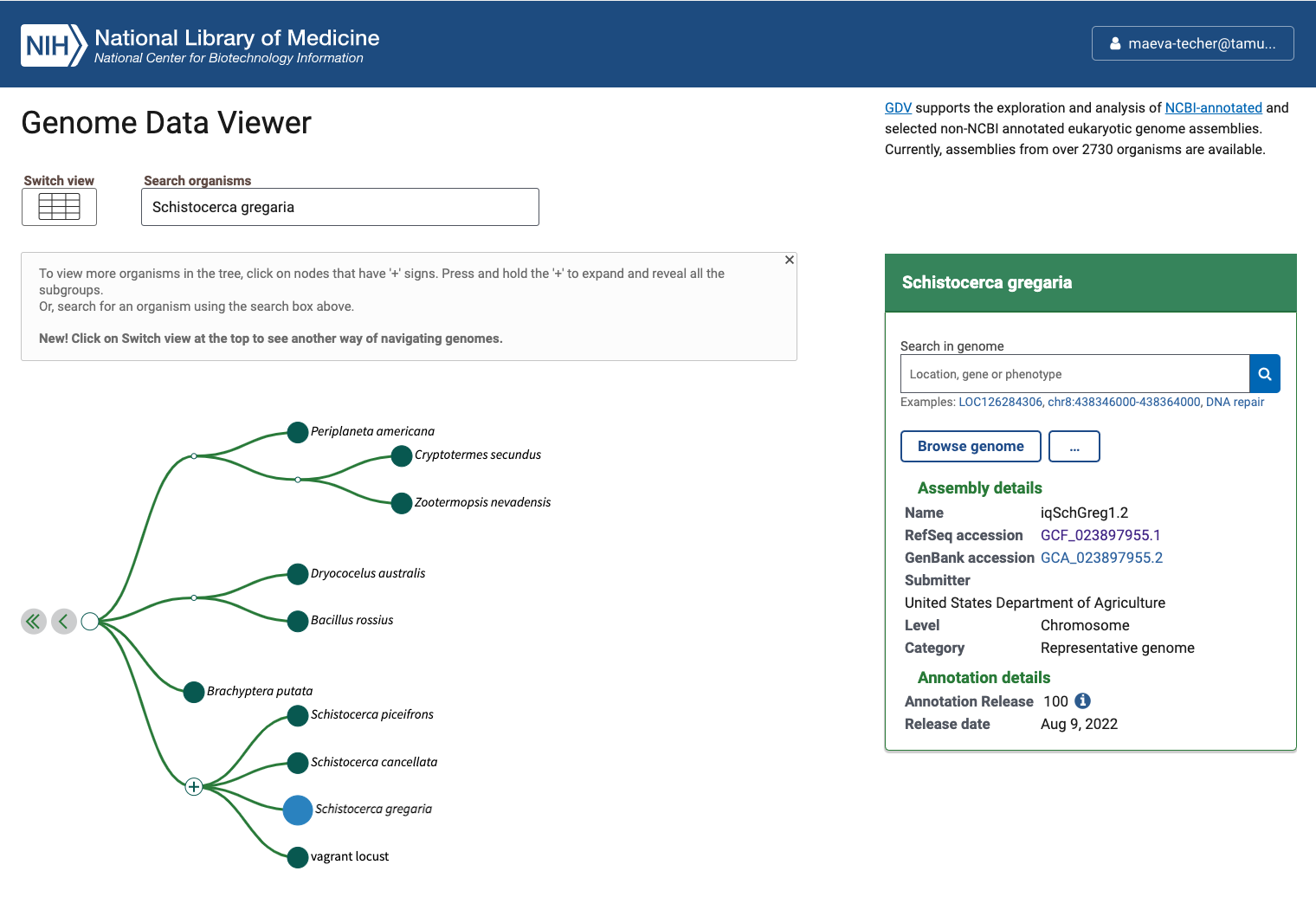
Status of Genome Data Viewer on NCBI for selecting our outgroups

NB: During our search, we identified very valuable genomes but for which no annotation was available (e.g., CAU_Lmig_1.0 for Locusta migratoria , iqMecThal1.2 Meconema thalassinum). However upon request to NCBI team, we were informed that the Locusta genome has not been annotated because of the presence of large bacterial contamination and Meconema does not possess RNA SRAs to help with the annotation.

Using the FTP NCBI link associated with each RefSeq, we created the input file.

./scripts/DataDownload ./scripts/inputurls_May2024.txt

On the TAMU Grace cluster, when you download do not run it on a node as it does not work. Run it from the login node or transfer the files already preloaded. This will creates a folder ./1_RawData with 3 files for each species.

In summary, below are the details of each RefSeq annotation that we will be using as input for OrthoFinder. It will be important to check that after steps 2-4, the number of protein coding genes OrthoFinder is similar to the initial input.


	Genomic Information of the RefSeq genomes used as input for OrthoFinder
Species	Order	Status	Genome_Size	Annotated_Genes	Protein_Coding
Schistocerca gregaria	Orthoptera	Locust	8.7 Gb	99467	19799
Schistocerca cancellata	Orthoptera	Locust	8.5 Gb	103533	16907
Schistocerca piceifrons	Orthoptera	Locust	8.7 Gb	96806	17490
Schistocerca americana	Orthoptera	Grasshopper	9.0 Gb	81274	17662
Schistocerca serialis cubense	Orthoptera	Grasshopper	9.1 Gb	75810	17237
Schistocerca nitens	Orthoptera	Grasshopper	8.8 Gb	72560	17500
Bacillus rossius redtenbacheri	Phasmatodea	Outgroup	1.6 Gb	19298	14448
Cryptotermes secundus	Blattodea	Outgroup	1.0 Gb	15413	13170
Apis mellifera	Hymenoptera	Outgroup	225.2 Mb	12398	9935
Solenopsis invicta	Hymenoptera	Outgroup	378.1 Mb	16996	14790
Acyrthosiphon pisum	Hemiptera	Outgroup	533.6 Mb	20307	17681
Drosophila melanogaster	Diptera	Outgroup	143.7 Mb	17872	13962

2. Selecting longest isoforms

Here again, we will follow the pipeline except that to run it on Grace cluster we will make small modifications. The idea is that we will use only the single longest isoform of each gene to ease the orthology analysis. While this might not always be the principal isoform of said gene, we will apply the same bias to all genes the same way.

First, to run R without bothering other users, we will claim one interactive node to make sure we can proactively update the package if there are some issues:

srun --ntasks 1 --cpus-per-task 4 --mem 10G --time 01:00:00 --pty bash

Then we will use any package preloaded on the cluster before needed to install our own on our user library if needed. We will need Pandoc for loading orthologr

ml GCC/12.2.0  OpenMPI/4.1.4 R_tamu/4.3.1
export R_LIBS=$SCRATCH/R_LIBS_USER/
ml Pandoc/2.13

We now simply run the script as indicated on the pipeline page:

./scripts/GeneRetrieval.R ./scripts/inputurls_May2024.txt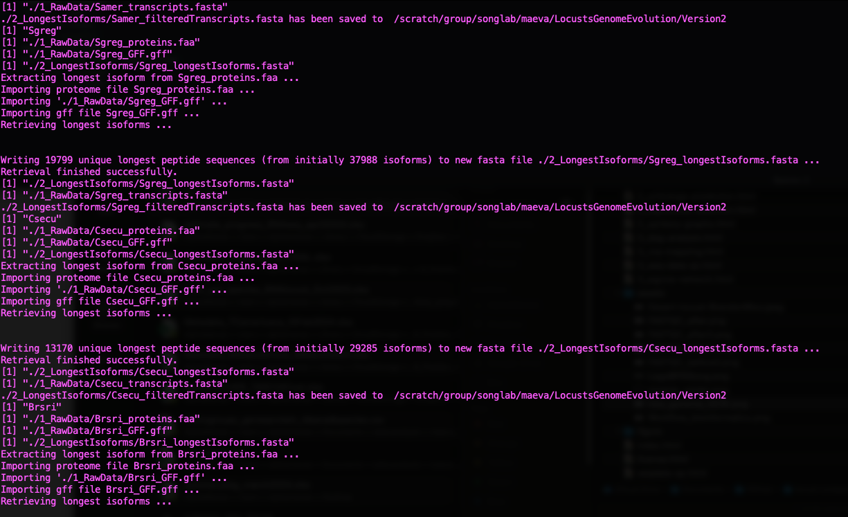

GeneRetrieval
Status of Gene Retrieval script when successful

Initially we wanted to also include the genome of Dryococelus australis (3.4Gb). However this will not be possible as the user submitted annotation does not match the need for orthologr here. There are some missing columns in the transcripts regarding “gene”.

3. Cleaning the raw data

For the cleaning step of the mbarkdull’s pipeline we simply followed the command line with no modifications.

./scripts/DataCleaning ./scripts/inputurls_May2024.txt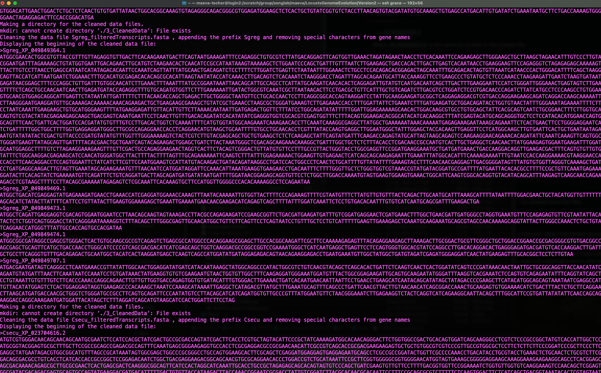

DataCleaning
Status of Data Cleaning script when successful

4. Translating nucleotide sequences to amino acid sequences

As mentioned in the pipeline page, we will mostly need to use amino acid sequences rather than protein and we need to translate the data we downloaded. We will be using the Python script from mbarkdull ./scripts/TranscriptFilesTranslateScript.py but before that we will modify our input file to only include only the 12 essential species.

We changed the script in head lines and lines 25-27, to call the module directly from the cluster as follow:

#!/bin/bash

##NECESSARY JOB SPECIFICATIONS
#SBATCH --job-name=Transdecoder         #Set the job name to "JobExample4"
#SBATCH --time=02:00:00         #Set the wall clock limit to 1hr and 30min
#SBATCH --ntasks=2              #Request 2 task
#SBATCH --cpus-per-task=4       #Request 8 task
#SBATCH --mem=20G              #Request 50GB per node

ml GCC/10.2.0 OpenMPI/4.0.5 TransDecoder/5.5.0 Biopython/1.78

   # Now we can run Transdecoder on the cleaned file:
    echo "First, attempting TransDecoder run on $cleanName"
    ml GCC/10.2.0 OpenMPI/4.0.5 TransDecoder/5.5.0
    TransDecoder.LongOrfs -t $cleanName
    TransDecoder.Predict -t $cleanName --single_best_only

and then we launched the script by changing the top lines to put in sbatch:

sbatch ./scripts/DataTranslating_modif ./scripts/inputurls_May2024.txt

5. Running Orthofinder

Now we will finally run Orthofinder to identify groups of orthologous genones in our translated amino acid sequences. We will also use MAFFT to produce multiple sequence alignment across our six species of Schistocerca and the outgroups.

Instead of using the ./scripts/DataOrthofinder from the pipeline, we will be running our own command line here. Before doing so, we did manually the creating of folders and moving of fasta files as follow:

  mkdir /LocustsGenomeEvolution/tmp
  mkdir ./5_OrthoFinder/fasta
  cp ./4_1_TranslatedData/OutputFiles/translated* ./5_OrthoFinder/fasta
  cd ./5_OrthoFinder/fasta
  rename translated '' translated*
  cd ../

To run orthofinder onto our Grace cluster, I checked the compatibility of the modules required and these are the versions acceptable to run in sbatchorthofinder.sh:

#!/bin/bash

##NECESSARY JOB SPECIFICATIONS
#SBATCH --job-name=orthofinder1         #Set the job name to "JobExample4"
#SBATCH --time=06:00:00         #Set the wall clock limit to 1hr and 30min
#SBATCH --ntasks=2              #Request 1 task
#SBATCH --cpus-per-task=4       #Request 1 task
#SBATCH --mem=30G              #Request 100GB per node

ml iccifort/2019.5.281  impi/2018.5.288 OrthoFinder/2.3.11-Python-3.7.4 
ml IQ-TREE/1.6.12 FastTree/2.1.11
ml MAFFT/7.453-with-extensions

orthofinder -S diamond -T iqtree -A mafft -I 5 -t 32 -a 4 -M msa -f /scratch/group/songlab/maeva/LocustsGenomeEvolution/Version2/5_OrthoFinder/fasta -p /scratch/group/songlab/maeva/LocustsGenomeEvolution/tmp

Here we use:
-S diamond DIAMOND as a sequence search program
-T iqtree IQTREE as a tree inference program
-A mafft MAFFT as the multiple sequence alignment (MSA) program
-I 5 MCL inflation parameter (default from the pipeline)
-t 32 number of threads

We want to run also orthofinder using BLAST as it can give -2% accuracy increase over DIAMOND but will be computationally more heavy. For this we will only change:

ml BLAST+/2.9.0
orthofinder -S blast

and we will run the script with the blast, iqtree and mafft options:

sbatch scripts/orthofinder_blast.sh

Now we are all done, we can explore the results and go on for the next steps.

6. Orthogroups to GeneID

At the end we obtain several folders, for which the content is extremely well explain by the software developer David Emms here.

Briefly, one of the important output in the folder Orthogroups is the actual Orthogroups.txt file. Although other files there are also important as we can use Orthogroups.GeneCount.tsv for CAFE5 later on, for example.

One of the issue with the pipeline we use is that, there will be some suffix in front of our protein coding, so we will remove that by using the following python code:

import re

# Define the input and output file names
input_file = 'Orthogroups.txt'
output_file = 'Orthogroups_reprocessed.txt'

# Read the input file
with open(input_file, 'r') as file:
    data = file.read()

# Remove all prefixes before any occurrence of "_XP", "_NP", and "_YP"
result = re.sub(r'\b\w+_(XP|NP|YP)', r'\1', data)

# Write the result to the output file
with open(output_file, 'w') as file:
    file.write(result)

print(f"Processed data has been written to {output_file}")

We used the python script protein2geneid_loop.py written by David to extract the protein_id from each gene_id and make a full table with all species. For this we need to run the script in the folder 1_RawData.

import os
import re

# Get the current working directory
gff_directory = os.getcwd()

# Create a directory to store the output files
output_directory = os.path.join(gff_directory, "output_files")
os.makedirs(output_directory, exist_ok=True)

# List GFF files with "_GFF.gff" extension
species_list = [filename for filename in os.listdir(gff_directory) if filename.endswith("_GFF.gff")]

# Process each species' GFF file
for species_filename in species_list:
    # Extract the species name from the file name
    species_name = re.sub(r"_GFF\.gff$", "", species_filename)
    
    # Construct input and output file paths
    input_path = os.path.join(gff_directory, species_filename)
    output_filename = f"xp{species_name}.gff"  # Remove the dot before species_name
    output_path = os.path.join(output_directory, output_filename)
    
    # Use 'grep' to filter lines containing "XP" and save to the output file
    grep_command = f'grep "XP" "{input_path}" > "{output_path}"'
    os.system(grep_command)
    
    # Print a message indicating the filtering process
    print(f"Filtered {species_filename} to {output_filename}")

    # Construct the output TSV file path
    tsv_output_filename = f'gffKey{species_name}.tsv'  # Remove the dot before species_name
    tsv_output_path = os.path.join(output_directory, tsv_output_filename)
    lol = {}

    # Read and process the contents of the GFF file
    with open(output_path) as gffFile:
        for line in gffFile:
            if re.search(r"product=[^;]+", line):
                gene_match = re.search(r"gene=[^;=]+", line)
                product_match = re.search(r"product=[^;]+", line)
                proteinID_match = re.search(r"protein_id=(.+)", line)
                
                if gene_match and product_match and proteinID_match:
                    gene = gene_match.group(0)
                    if gene.endswith('product'):
                        gene = gene[5:-7]
                    else:
                        gene = gene[5:]
                    
                    product = product_match.group(0)
                    product = product.replace("product=", "")
                    product = product.rstrip()
                    
                    proteinID = proteinID_match.group(1)
                    
                    if proteinID not in lol.keys():
                        lol[proteinID] = [gene, product, species_name]  # Add species name

    # Write the processed data to the output TSV file
    with open(tsv_output_path, 'w') as output:
        for proID, lis in lol.items():
            output.writelines(proID + '\t' + lis[0] + '\t' + lis[1] + '\t' + lis[2] + '\n')  # Include species name

    # Print a message indicating the processing of the GFF file
    print(f"Processed {output_filename} to {tsv_output_filename}")

# Concatenate all final files into a single file
final_output_filename = "allspecies_protein2geneid.tsv"
final_output_path = os.path.join(output_directory, final_output_filename)

with open(final_output_path, 'w') as final_output:
    for species_filename in species_list:
        species_name = re.sub(r"_GFF\.gff$", "", species_filename)
        tsv_output_filename = f'gffKey{species_name}.tsv'  # Remove the dot before species_name
        tsv_output_path = os.path.join(output_directory, tsv_output_filename)
        
        with open(tsv_output_path, 'r') as species_output:
            final_output.write(species_output.read())

print(f"Concatenated all species files into {final_output_filename}")

Launch the script as python protein2geneid_loop.py.

Once we have obtained both files, we can join them with R and we will have a correspondence among orthogroups_id, protein_id, gene_id, gene description and species.

NB: I noticed there are still some small issues with teh file allspecies_protein2geneid.tsv so I fixed it by hand afterwards.

library(readr)
library(tidyverse)

orthogroup <- read_table("data/orthologs/Orthogroups_reprocessed.txt", col_names = FALSE)

# We reshape the table so that we have one orthogroup line associated with one protein id
transformed_orthogroup <- orthogroup %>%
  pivot_longer(cols = -X1, names_to = "Protein_Column", values_to = "protein_id") %>%
  replace_na(list(X1 = "N/A")) %>%
  select(orthogroup = X1, protein_id) %>%
  filter(!is.na(protein_id))

# Export the table to  tab-separated text file (you can change the delimiter if needed)
write.table(transformed_orthogroup, file = "data/orthologs/Orthogroups_11species_May2024.txt", sep = "\t", quote = FALSE, row.names = FALSE)

proteingeneid <- read_tsv("data/orthologs/allspecies_protein2geneid.tsv", col_names = TRUE ) 

final_orthotable <- left_join(transformed_orthogroup, proteingeneid, by = "protein_id")
write.table(final_orthotable, file = "data/orthologs/Orthogroups_genesprotein_11species_May2024.csv", sep = ",", quote = FALSE, row.names = FALSE)

There we have it, the final table with all the corresponding IDs.

library(readr)
library(tidyverse)

fulltable <- read_csv("data/orthologs/Orthogroups_genesprotein_11species_May2024.csv", col_names = TRUE)
view(fulltable)

References

If you use this script, and orthologr please cite:

Drost et al. 2015. Evidence for Active Maintenance of Phylotranscriptomic Hourglass Patterns in Animal and Plant Embryogenesis. Mol. Biol. Evol. 32 (5): 1221-1231. doi:10.1093/molbev/msv012

If you use Transdecoder, please cite it as:

Haas, B., and A. Papanicolaou. “TransDecoder.” (2017).

If you use Orthofinder, please cite it:

OrthoFinder’s orthogroup and ortholog inference are described here:

Emms, D.M., Kelly, S. OrthoFinder: solving fundamental biases in whole genome comparisons dramatically improves orthogroup inference accuracy. Genome Biol 16, 157 (2015).

Emms, D.M., Kelly, S. OrthoFinder: phylogenetic orthology inference for comparative genomics. Genome Biol 20, 238 (2019).

If you use the OrthoFinder species tree then also cite:

Emms D.M. & Kelly S. STRIDE: Species Tree Root Inference from Gene Duplication Events (2017), Mol Biol Evol 34(12): 3267-3278.

Emms D.M. & Kelly S. STAG: Species Tree Inference from All Genes (2018), bioRxiv https://doi.org/10.1101/267914.

Please also cite MAFFT:

K. Katoh, K. Misawa, K. Kuma, and T. Miyata. 2002. MAFFT: a novel method for rapid multiple sequence alignment based on fast Fourier transform. Nucleic Acids Res. 30(14): 3059-3066.

sessionInfo()

R version 4.4.1 (2024-06-14)
Platform: aarch64-apple-darwin20
Running under: macOS Sonoma 14.7

Matrix products: default
BLAS:   /Library/Frameworks/R.framework/Versions/4.4-arm64/Resources/lib/libRblas.0.dylib 
LAPACK: /Library/Frameworks/R.framework/Versions/4.4-arm64/Resources/lib/libRlapack.dylib;  LAPACK version 3.12.0

locale:
[1] en_US.UTF-8/en_US.UTF-8/en_US.UTF-8/C/en_US.UTF-8/en_US.UTF-8

time zone: Asia/Tokyo
tzcode source: internal

attached base packages:
[1] stats     graphics  grDevices utils     datasets  methods   base     

other attached packages:
[1] kableExtra_1.4.0 knitr_1.48      

loaded via a namespace (and not attached):
 [1] jsonlite_1.8.9    highr_0.11        compiler_4.4.1    promises_1.3.0   
 [5] Rcpp_1.0.13       xml2_1.3.6        stringr_1.5.1     git2r_0.35.0     
 [9] later_1.3.2       jquerylib_0.1.4   systemfonts_1.1.0 scales_1.3.0     
[13] yaml_2.3.10       fastmap_1.2.0     R6_2.5.1          workflowr_1.7.1  
[17] tibble_3.2.1      munsell_0.5.1     rprojroot_2.0.4   svglite_2.1.3    
[21] bslib_0.8.0       pillar_1.9.0      rlang_1.1.4       utf8_1.2.4       
[25] cachem_1.1.0      stringi_1.8.4     httpuv_1.6.15     xfun_0.49        
[29] fs_1.6.5          sass_0.4.9        viridisLite_0.4.2 cli_3.6.3        
[33] magrittr_2.0.3    digest_0.6.37     rstudioapi_0.17.1 lifecycle_1.0.4  
[37] vctrs_0.6.5       evaluate_1.0.1    glue_1.8.0        whisker_0.4.1    
[41] fansi_1.0.6       colorspace_2.1-1  rmarkdown_2.28    tools_4.4.1      
[45] pkgconfig_2.0.3   htmltools_0.5.8.1

Orthology inference: How are genes related across Schistocerca species?

Maeva Techer

2024-11-01