Last updated: 2025-04-10

Checks: 6 1

Knit directory: HairCort-Evaluation-Nist2020/

This reproducible R Markdown analysis was created with workflowr (version 1.7.1). The Checks tab describes the reproducibility checks that were applied when the results were created. The Past versions tab lists the development history.

R Markdown file: uncommitted changes

The R Markdown file has unstaged changes. To know which version of the R Markdown file created these results, you’ll want to first commit it to the Git repo. If you’re still working on the analysis, you can ignore this warning. When you’re finished, you can run wflow_publish to commit the R Markdown file and build the HTML.

Environment: empty

Great job! The global environment was empty. Objects defined in the global environment can affect the analysis in your R Markdown file in unknown ways. For reproduciblity it’s best to always run the code in an empty environment.

Seed: set.seed(20241016)

The command set.seed(20241016) was run prior to running the code in the R Markdown file. Setting a seed ensures that any results that rely on randomness, e.g. subsampling or permutations, are reproducible.

Session information: recorded

Great job! Recording the operating system, R version, and package versions is critical for reproducibility.

Cache: none

Nice! There were no cached chunks for this analysis, so you can be confident that you successfully produced the results during this run.

File paths: relative

Great job! Using relative paths to the files within your workflowr project makes it easier to run your code on other machines.

Repository version: bbb70a9

Great! You are using Git for version control. Tracking code development and connecting the code version to the results is critical for reproducibility.

The results in this page were generated with repository version bbb70a9. See the Past versions tab to see a history of the changes made to the R Markdown and HTML files.

Note that you need to be careful to ensure that all relevant files for the analysis have been committed to Git prior to generating the results (you can use wflow_publish or wflow_git_commit). workflowr only checks the R Markdown file, but you know if there are other scripts or data files that it depends on. Below is the status of the Git repository when the results were generated:


Ignored files:
    Ignored:    .DS_Store
    Ignored:    .RData
    Ignored:    .Rhistory
    Ignored:    analysis/.DS_Store
    Ignored:    analysis/.Rhistory
    Ignored:    data/.DS_Store
    Ignored:    data/Test3/.DS_Store
    Ignored:    data/Test4/.DS_Store

Untracked files:
    Untracked:  analysis/ELISA_Analysis_FinalVals_comparisons_test3_test4.Rmd

Unstaged changes:
    Deleted:    ELISA_Analysis_FinalVals_comparisons_test3_test4.Rmd
    Deleted:    ELISA_Analysis_FinalVals_comparisons_test3_test4.html
    Modified:   analysis/ELISA_Analysis_RawVals_test3.Rmd
    Modified:   analysis/ELISA_Analysis_RawVals_test4.Rmd
    Modified:   analysis/ELISA_Calc_FinalVals_test3.Rmd
    Modified:   analysis/ELISA_Calc_FinalVals_test4.Rmd
    Modified:   analysis/ELISA_QC_test4.Rmd
    Modified:   data/Test4/Data_QC_filtered.csv
    Modified:   data/Test4/Data_QC_flagged.csv
    Modified:   data/Test4/Data_cort_values_methodA.csv
    Modified:   data/Test4/Data_cort_values_methodB.csv
    Modified:   data/Test4/Data_cort_values_methodC.csv
    Modified:   data/Test4/Data_cort_values_methodD.csv
    Modified:   data/Test4/failed_samples.csv
    Deleted:    temp.html

Note that any generated files, e.g. HTML, png, CSS, etc., are not included in this status report because it is ok for generated content to have uncommitted changes.

These are the previous versions of the repository in which changes were made to the R Markdown (analysis/ELISA_Calc_FinalVals_test4.Rmd) and HTML (docs/ELISA_Calc_FinalVals_test4.html) files. If you’ve configured a remote Git repository (see ?wflow_git_remote), click on the hyperlinks in the table below to view the files as they were in that past version.

File	Version	Author	Date	Message
html	bbb70a9	Paloma	2025-04-09	comparing methods
Rmd	ccad031	Paloma	2025-04-09	new_calc
html	ccad031	Paloma	2025-04-09	new_calc
html	77c2ab5	Paloma	2025-04-08	cleaning test3
Rmd	ced6eed	Paloma	2025-04-03	upd
html	ced6eed	Paloma	2025-04-03	upd
Rmd	ca6c804	Paloma	2025-04-03	new calc final vals
html	ca6c804	Paloma	2025-04-03	new calc final vals
Rmd	528855b	Paloma	2025-04-03	new_calc
html	528855b	Paloma	2025-04-03	new_calc

Summary

Cortisol value calculations

	Min.	1st Qu.	Median	Mean	3rd Qu.	Max.	NA’s
A) Standard Method	0.4142	1.9653	7.5533	14.1906	28.0667	50.933	3
B) Spike-Corrected Method	-45.870	-31.922	-1.929	-9.444	7.553	30.780	3
C) Standard, but simplified equation	0.4142	1.9653	7.5533	14.1906	28.0667	50.9333	3
D) Spike-Corrected (divided by two)	0.2335	1.5067	6.7184	9.7699	17.3683	32.2815	3

I calculated final cortisol values in pg/mg using the following key variables:

Ave_Conc_pg/ml: average ELISA reading per sample in pg/mL
Weight_mg: hair weight in mg
Buffer_nl: assay buffer volume in nL → we convert to mL
Spike: binary indicator (1 = spiked sample)
SpikeVol_uL: volume of spike added in µL
Dilution: dilution factor (already present)
Vol_in_well.tube_uL: total volume in well/tube in µL (for spike correction)
std: standard reading value
extraction: methanol volume ratio = vol added / vol recovered (1/0.75 ml)

Results:

Intra-assay CV: 14.5%
Intra-assay CV after removing low quality samples: 10%
Inter-assay CV: 21%

(Bindings for 20mg sample diluted in 250 uL, no spike: 64.8% and 48% in test3 and test4, respectively)

Conclusions:

Concerns: Overall quality of the plate is not great, but serial dilusions show clear parallelism and standards have values within the expected

Cortisol concentration calculations

# set reading value of spike (std1, 0.333 ug/dL), 
# and transforming to ug.dL

std <- (3191+3228)/2
std.r <- (std/10000)
std

[1] 3209.5

std.r

[1] 0.32095

# according to chatgpt, the spike's contribution is
# 1600 pg/mL, which is very similar to half of the reading for std 1 :]

Loading files and transforming units, including low quality data

df <- read.csv(file.path(data_path,"Data_QC_flagged.csv"))
kable(tail(df))

	Wells	Sample	Category	Weight_mg	Buffer_nl	Spike	SpikeVol_uL	Dilution_sample	Dilution_spike	Vol_in_well.tube_uL	Extraction_ratio	Raw.OD	Binding.Perc	Conc_pg.ml	Ave_Conc_pg.ml	CV.Perc	SD	SEM	CV_categ	Binding.Perc_categ	Failed_samples
77	G11	TP3A	P	12	220	1	25	1	1	50	1.351351	0.258	23.2	2800	2792	0.391	10.9	7.71	NA	NA	NA
78	H11	TP3A	P	12	220	1	25	1	1	50	1.351351	0.259	NA	2785	NA	NA	NA	NA	NA	NA	NA
79	A12	TP3B	P	12	60	1	25	1	1	50	1.333333	0.195	15.5	4084	4210	4.230	178.0	126.00	NA	UNDER 20% binding	UNDER 20% binding
80	B12	TP3B	P	12	60	1	25	1	1	50	1.333333	0.186	NA	4336	NA	NA	NA	NA	NA	NA	NA
81	C12	TP3C	P	12	60	1	25	1	1	50	1.333333	0.186	13.9	4336	4661	9.870	460.0	325.00	NA	UNDER 20% binding	UNDER 20% binding
82	D12	TP3C	P	12	60	1	25	1	1	50	1.333333	0.166	NA	4986	NA	NA	NA	NA	NA	NA	NA

# remove outlier
#df<- df[(df$Sample != "TP3A"),]

# Creating variables in indicated units
# dilution (buffer)
df$Buffer_ml <- c(df$Buffer_nl/1000)
df$Failed_samples[is.na(df$Failed_samples)] <- "OK"
table(df$Failed_samples)


        ABOVE 80% binding                   HIGH CV HIGH CV;ABOVE 80% binding 
                        4                         2                         7 
HIGH CV;UNDER 20% binding                        OK         UNDER 20% binding 
                        1                        60                         8

df$Failed_samples[df$Failed_samples == "ABOVE 80% binding"] <- "Out of curve"
df$Failed_samples[df$Failed_samples == "HIGH CV;ABOVE 80% binding"] <- "High CV & Out of curve"
df$Failed_samples[df$Failed_samples == "HIGH CV;UNDER 20% binding"] <- "High CV & Out of curve"
df$Failed_samples[df$Failed_samples == "HIGH CV"] <- "High CV"
df$Failed_samples[df$Failed_samples == "UNDER 20% binding"] <- "Out of curve"

df$Failed_samples <- factor(
  df$Failed_samples,
  levels = c(
    "OK",
    "Out of curve",
    "High CV",
    "High CV & Out of curve"
  )
)



# remove unnecessary information 
data <- df %>%
    dplyr::select(Wells, Sample, Category, Binding.Perc, Ave_Conc_pg.ml, Weight_mg, Buffer_ml, Spike, SpikeVol_uL, Dilution_sample, Dilution_spike, Extraction_ratio, Vol_in_well.tube_uL, Failed_samples) 



# remove duplicates
data <- data[!is.na(data$Binding.Perc), ]

kable(tail(data, 10))

	Wells	Sample	Category	Binding.Perc	Ave_Conc_pg.ml	Weight_mg	Buffer_ml	Spike	SpikeVol_uL	Dilution_sample	Dilution_spike	Extraction_ratio	Vol_in_well.tube_uL	Failed_samples
63	A10	TD7	D	99.0	86.73	20	0.11	1	110	64	64	1.333333	220	Out of curve
65	C10	TP1A	P	21.8	2986.00	6	0.06	1	25	1	1	1.333333	50	OK
67	E10	TP1B	P	18.1	3820.00	6	0.06	1	25	1	1	1.333333	50	High CV & Out of curve
69	G10	TP1C*FAIL	P	27.8	2242.00	6	0.06	1	25	1	1	1.851852	50	OK
71	A11	TP2A	P	17.3	3793.00	9	0.06	1	25	1	1	1.333333	50	Out of curve
73	C11	TP2B	P	21.1	3101.00	9	0.06	1	25	1	1	1.333333	50	OK
75	E11	TP2C	P	18.1	3634.00	9	0.06	1	25	1	1	1.333333	50	Out of curve
77	G11	TP3A	P	23.2	2792.00	12	0.22	1	25	1	1	1.351351	50	OK
79	A12	TP3B	P	15.5	4210.00	12	0.06	1	25	1	1	1.333333	50	Out of curve
81	C12	TP3C	P	13.9	4661.00	12	0.06	1	25	1	1	1.333333	50	Out of curve

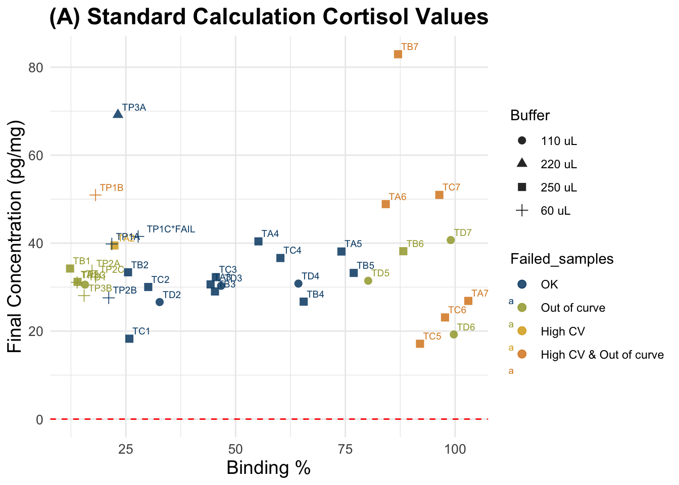
dim(data)

[1] 41 14

(A) Standard Calculation

Formula:

((A/B) * (C/D) * E * 10,000) = F

A = μg/dl from assay output;
B = weight (in mg) of hair subjected to extraction;
C = vol. (in ml) of methanol added to the powdered hair;
D = vol. (in ml) of methanol recovered from the extract and subsequently dried down;
E = vol. (in ml) of assay buffer used to reconstitute the dried extract;
F = final value of hair CORT Concentration in pg/mg.

##################################
##### Calculate final values #####
##################################

# Transform to μg/dl from assay output
data$Ave_Conc_ug.dL <- c(data$Ave_Conc_pg.ml/10000)

data$Final_conc_pg.mg <- c(
    ((data$Ave_Conc_ug.dL) / data$Weight_mg) * # A/B *
      data$Extraction_ratio *                                  # C/D  *     
      data$Buffer_ml * 10000 * data$Dilution_sample)                 # E * 10000
data <- data[order(data$Sample),]
write.csv(data, file.path(data_path, "Data_cort_values_methodA.csv"), row.names = F)

# summary for all samples
summary(data$Final_conc_pg.mg)

   Min. 1st Qu.  Median    Mean 3rd Qu.    Max.    NA's 
  17.13   29.01   32.27   35.28   39.47   82.94       4

kable(tail(data, 7))

	Wells	Sample	Category	Binding.Perc	Ave_Conc_pg.ml	Weight_mg	Buffer_ml	Spike	SpikeVol_uL	Dilution_sample	Dilution_spike	Extraction_ratio	Vol_in_well.tube_uL	Failed_samples	Ave_Conc_ug.dL	Final_conc_pg.mg
69	G10	TP1C*FAIL	P	27.8	2242	6	0.06	1	25	1	1	1.851852	50	OK	0.2242	41.51852
71	A11	TP2A	P	17.3	3793	9	0.06	1	25	1	1	1.333333	50	Out of curve	0.3793	33.71556
73	C11	TP2B	P	21.1	3101	9	0.06	1	25	1	1	1.333333	50	OK	0.3101	27.56444
75	E11	TP2C	P	18.1	3634	9	0.06	1	25	1	1	1.333333	50	Out of curve	0.3634	32.30222
77	G11	TP3A	P	23.2	2792	12	0.22	1	25	1	1	1.351351	50	OK	0.2792	69.17117
79	A12	TP3B	P	15.5	4210	12	0.06	1	25	1	1	1.333333	50	Out of curve	0.4210	28.06667
81	C12	TP3C	P	13.9	4661	12	0.06	1	25	1	1	1.333333	50	Out of curve	0.4661	31.07333

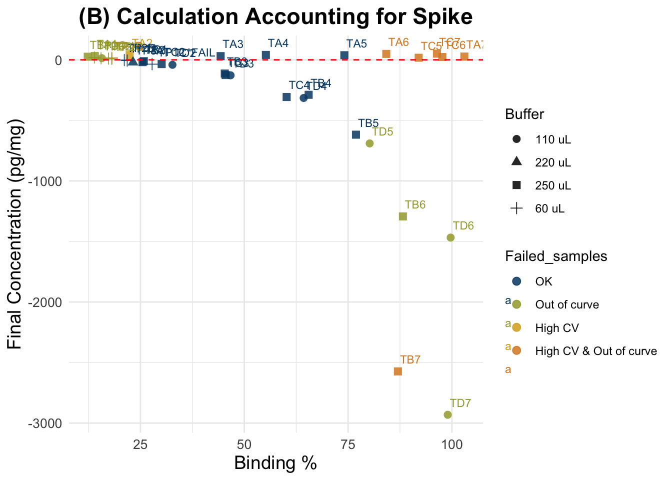
dim(data)

[1] 41 16

(B) Accounting for Spike

We followed the procedure described in Nist et al. 2020:

“Thus, after pipetting 25μL of standards and samples into the appropriate wells of the 96-well assay plate, we added 25μL of the 0.333ug/dL standard to all samples, resulting in a 1:2 dilution of samples. The remainder of the manufacturer’s protocol was unchanged. We analyzed the assay plate in a Powerwave plate reader (BioTek, Winooski, VT) at 450nm and subtracted background values from all assay wells. In the calculations, we subtracted the 0.333ug/dL standard reading from the sample readings. Samples that resulted in a negative number were considered nondetectable. We converted cortisol levels from ug/dL, as measured by the assay, to pg/mg—based on the mass of hair collected and analyzed using the following formula:

A/B * C/D * E * 10,000 * 2 = F

where - A = μg/dl from assay output; - B = weight (in mg) of collected hair; - C = vol. (in ml) of methanol added to the powdered hair; - D = vol. (in ml) of methanol recovered from the extract and subsequently dried down; - E = vol. (in ml) of assay buffer used to reconstitute the dried extract; 10,000 accounts for changes in metrics; 2 accounts for the dilution factor after addition of the spike; and - F = final value of hair cortisol concentration in pg/mg”

dSpike <- data

##################################
##### Calculate final values #####
##################################

dSpike$Final_conc_pg.mg <- 
  ifelse(
    dSpike$Spike == 1,    ## Only spiked samples
      ((dSpike$Ave_Conc_ug.dL - (std.r)) / # (A-spike) / B
        dSpike$Weight_mg) 
        * data$Extraction_ratio *                  # C / D
        dSpike$Buffer_ml * 10000 * 2 * dSpike$Dilution_sample,    # E * 10000 * 2
        dSpike$Final_conc_pg.mg  
    )


write.csv(dSpike, file.path(data_path, "Data_cort_values_methodB.csv"), row.names = F)

# summary for all samples
summary(dSpike$Final_conc_pg.mg)

    Min.  1st Qu.   Median     Mean  3rd Qu.     Max.     NA's 
-2931.24  -127.69    -5.96  -285.62    23.11    50.96        4

dSpikeSub <- data[c(data$Spike == 0), ]
summary(dSpikeSub$Final_conc_pg.mg)

   Min. 1st Qu.  Median    Mean 3rd Qu.    Max.    NA's 
  17.13   27.81   34.65   34.67   40.17   50.96       4

kable(tail(dSpike, 10))

	Wells	Sample	Category	Binding.Perc	Ave_Conc_pg.ml	Weight_mg	Buffer_ml	Spike	SpikeVol_uL	Dilution_sample	Dilution_spike	Extraction_ratio	Vol_in_well.tube_uL	Failed_samples	Ave_Conc_ug.dL	Final_conc_pg.mg
63	A10	TD7	D	99.0	86.73	20	0.11	1	110	64	64	1.333333	220	Out of curve	0.008673	-2931.240106
65	C10	TP1A	P	21.8	2986.00	6	0.06	1	25	1	1	1.333333	50	OK	0.298600	-5.960000
67	E10	TP1B	P	18.1	3820.00	6	0.06	1	25	1	1	1.333333	50	High CV & Out of curve	0.382000	16.280000
69	G10	TP1C*FAIL	P	27.8	2242.00	6	0.06	1	25	1	1	1.851852	50	OK	0.224200	-35.833333
71	A11	TP2A	P	17.3	3793.00	9	0.06	1	25	1	1	1.333333	50	Out of curve	0.379300	10.373333
73	C11	TP2B	P	21.1	3101.00	9	0.06	1	25	1	1	1.333333	50	OK	0.310100	-1.928889
75	E11	TP2C	P	18.1	3634.00	9	0.06	1	25	1	1	1.333333	50	Out of curve	0.363400	7.546667
77	G11	TP3A	P	23.2	2792.00	12	0.22	1	25	1	1	1.351351	50	OK	0.279200	-20.686937
79	A12	TP3B	P	15.5	4210.00	12	0.06	1	25	1	1	1.333333	50	Out of curve	0.421000	13.340000
81	C12	TP3C	P	13.9	4661.00	12	0.06	1	25	1	1	1.333333	50	Out of curve	0.466100	19.353333

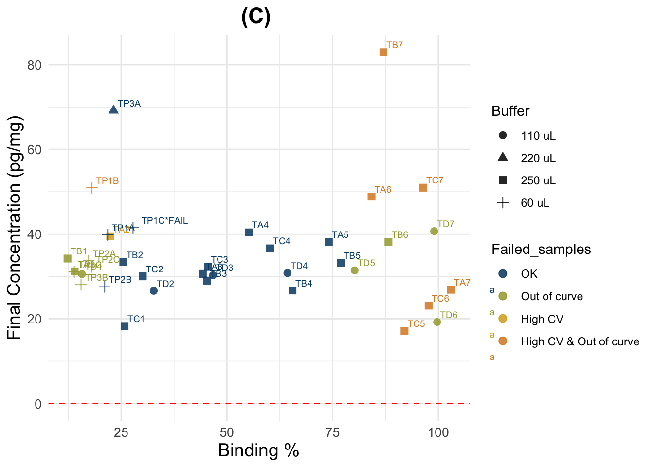
(C) Skip unit transformation

##################################
##### Calculate final values #####
################################## 
datac <- data
datac$Final_conc_pg.mg <- c(
    (datac$Ave_Conc_pg.ml / datac$Weight_mg) * # A/B *
     data$Extraction_ratio *                                  # C/D  *     
      datac$Buffer_ml * datac$Dilution_sample)                 # E 
datac <- datac[order(datac$Sample),]
write.csv(datac, file.path(data_path, "Data_cort_values_methodC.csv"), row.names = F)

# summary for all samples
summary(datac$Final_conc_pg.mg)

   Min. 1st Qu.  Median    Mean 3rd Qu.    Max.    NA's 
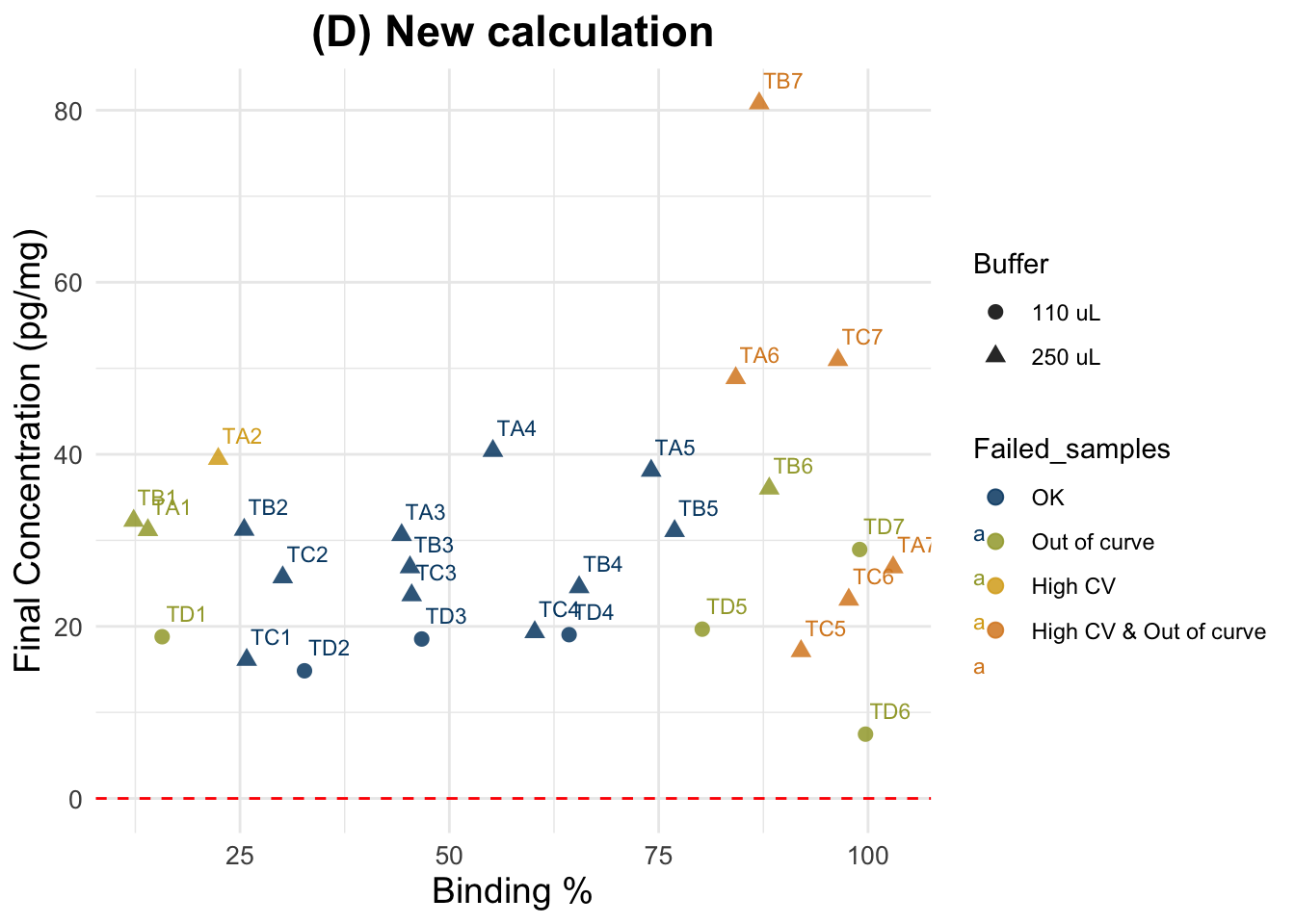
  17.13   29.01   32.27   35.28   39.47   82.94       4

(D) Account for Spike contribution (uses vol. of spike, conc. of spike, and total reconstit. vol.)

Spike contribution (pg/mL) = (Vol. spike (mL) x Conc. spike (pg/mL) ) / Vol. reconstitution (mL) or total vol. in well (50uL) (depending on where the spike was added)

# Calculate contribution of spike according to the different volumes in which it was added
# Consider that contribution of spike in serial dilutions gets smaller 

# Vol. of spike transformed to mL
data$SpikeVol_ml <- data$SpikeVol_uL/1000
# Concentration of the spike:
std

[1] 3209.5

# Vol. reconstitution (mL) is the total volume in tube or well (sample + spike), after adding spike.
# transform to mL
data$Vol_in_well.tube_ml <- data$Vol_in_well.tube_uL/1000


  ##( Spike vol. x Spike Conc.)
  ## ------------------------  / dilution = Spike contribution
  ##      Total vol. 
  
# Cortisol added by spike in wells: 0.0025 mL x 3200 pg/mL = 80 pg
# Calculate cort contribution of spike to each sample
data$Spike.cont_pg.mL <- ((data$SpikeVol_ml * std  / # Volume of spike * Spike concentration
                            data$Vol_in_well.tube_ml) / # divided by the total volume (spike + sample)
                              data$Dilution_spike) # resulting number changes depending on the dilution

dSpiked <- data
                          
##################################
##### Calculate final values #####
##################################


dSpiked$Final_conc_pg.mg <- 
     (((dSpiked$Ave_Conc_pg.ml - dSpiked$Spike.cont_pg.mL)) / # (A - spike) / B
      dSpiked$Weight_mg) *
     dSpiked$Extraction_ratio *      # C / D
      dSpiked$Buffer_ml * dSpiked$Dilution_sample    # E * 



write.csv(dSpiked, file.path(data_path, "Data_cort_values_methodD.csv"), row.names = F)

# summary for all samples
summary(dSpiked$Final_conc_pg.mg)

   Min. 1st Qu.  Median    Mean 3rd Qu.    Max.    NA's 
  7.472  18.533  24.559  27.009  31.196  80.804       4

kable(head(dSpiked[!is.na(dSpiked$Final_conc_pg.mg) , c("Sample", "Final_conc_pg.mg", "Ave_Conc_pg.ml", "Spike.cont_pg.mL", "Binding.Perc", "Weight_mg", "Buffer_ml", "SpikeVol_uL", "Dilution_sample", "Dilution_spike", "Vol_in_well.tube_uL", "Extraction_ratio")],10))

	Sample	Final_conc_pg.mg	Ave_Conc_pg.ml	Spike.cont_pg.mL	Binding.Perc	Weight_mg	Buffer_ml	SpikeVol_uL	Dilution_sample	Dilution_spike	Vol_in_well.tube_uL	Extraction_ratio
9	TA1	31.19595	4617.00	0.0000	14.0	50	0.25	0	1	1	50	1.351351
11	TA2	39.47297	2921.00	0.0000	22.4	50	0.25	0	2	1	50	1.351351
13	TA3	30.62162	1133.00	0.0000	44.3	50	0.25	0	4	1	50	1.351351
15	TA4	40.40000	747.40	0.0000	55.2	50	0.25	0	8	1	50	1.351351
17	TA5	38.09730	352.40	0.0000	74.1	50	0.25	0	16	1	50	1.351351
19	TA6	48.86486	226.00	0.0000	84.2	50	0.25	0	32	1	50	1.351351
21	TA7	26.86703	62.13	0.0000	103.0	50	0.25	0	64	1	50	1.351351
23	TB1	32.28152	5134.00	291.7727	12.3	50	0.25	25	1	1	275	1.333333
25	TB2	31.23367	2503.00	160.4750	25.5	50	0.25	25	2	2	250	1.333333
27	TB3	26.87367	1088.00	80.2375	45.3	50	0.25	25	4	4	250	1.333333

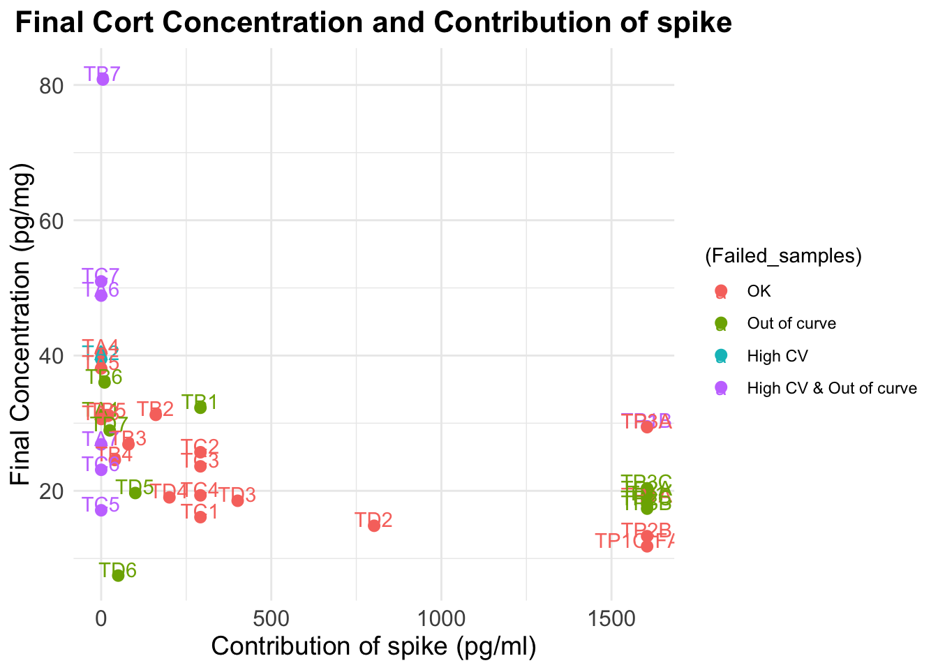
Plots

(A) Standard Calculation

Version	Author	Date
ccad031	Paloma	2025-04-09
ced6eed	Paloma	2025-04-03

(B) Accounting for Spike

Version	Author	Date
ccad031	Paloma	2025-04-09
ced6eed	Paloma	2025-04-03

(C) Simplified Standard Calculation

Version	Author	Date
ccad031	Paloma	2025-04-09
ced6eed	Paloma	2025-04-03

(D) New calculation (substract half of the spike from A)

Version	Author	Date
ccad031	Paloma	2025-04-09
ced6eed	Paloma	2025-04-03

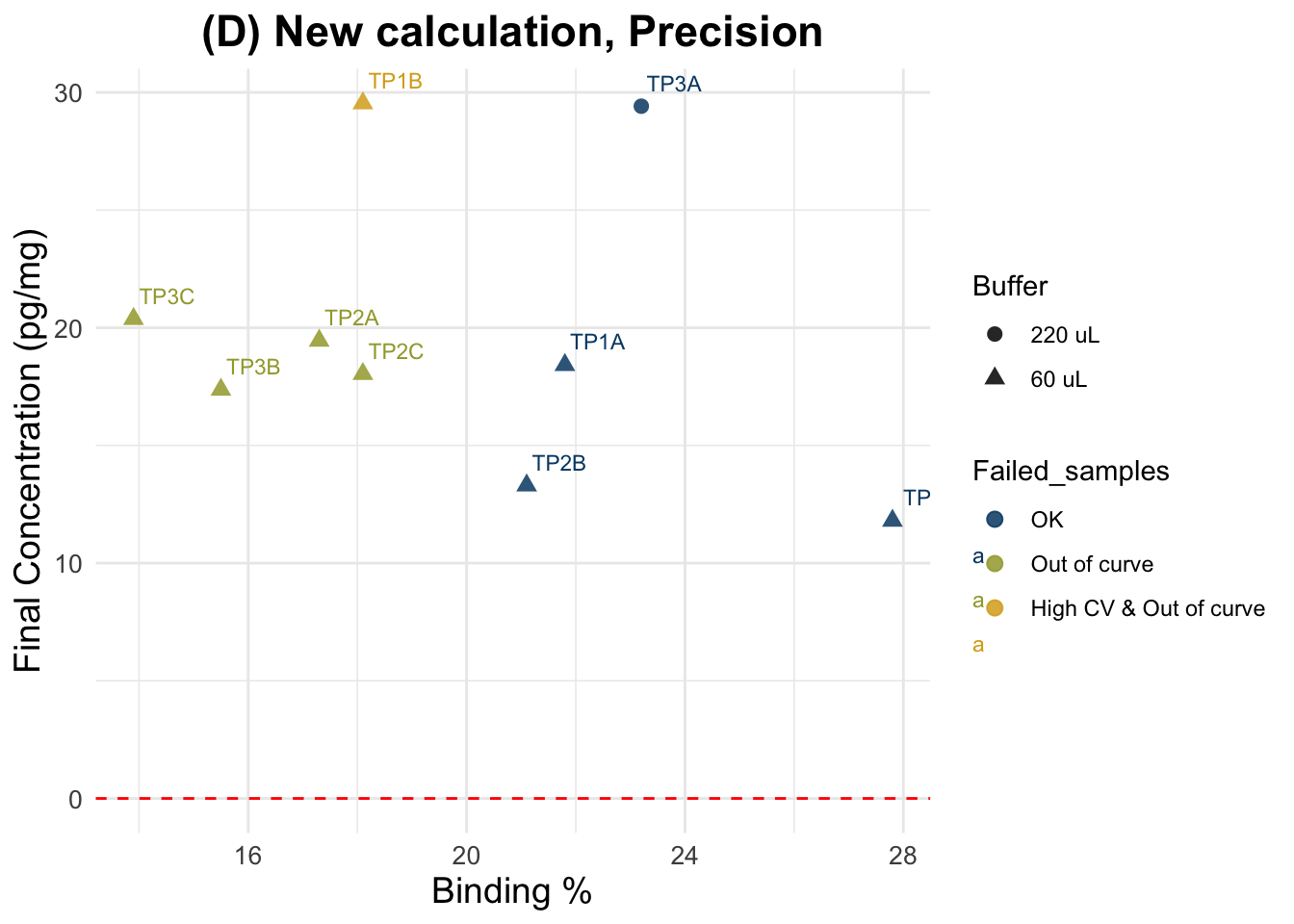
Evaluation

Since all spiked samples produce negative values, we will continue our analyses using only non-spiked samples.

ggplot(dSpiked, aes(y = Final_conc_pg.mg, 
                  x = Spike.cont_pg.mL, 
                  color = (Failed_samples))) + 
                 # fill = factor(Spike.cont_pg.mL))) +
  geom_point(size = 2.5) +  
  geom_text(label = c(dSpiked$Sample), nudge_y = 0.95, nudge_x = -1.2) +
 # geom_hline(yintercept = mean(data$Final_conc_pg.mg), 
  #           color = "gray80",
   #          linetype = "dashed") +
  theme_minimal() +  
  labs(
    title = "Final Cort Concentration and Contribution of spike",
    y = "Final Concentration (pg/mg)",
    x = "Contribution of spike (pg/ml)"  
  ) +
  theme(
    plot.title = element_text(hjust = 0.5, size = 16, face = "bold"),  
    axis.title = element_text(size = 14),  
    axis.text = element_text(size = 12) 
  )

Version	Author	Date
ccad031	Paloma	2025-04-09
ced6eed	Paloma	2025-04-03
528855b	Paloma	2025-04-03

sessionInfo()

R version 4.4.3 (2025-02-28)
Platform: aarch64-apple-darwin20
Running under: macOS Sequoia 15.4

Matrix products: default
BLAS:   /Library/Frameworks/R.framework/Versions/4.4-arm64/Resources/lib/libRblas.0.dylib 
LAPACK: /Library/Frameworks/R.framework/Versions/4.4-arm64/Resources/lib/libRlapack.dylib;  LAPACK version 3.12.0

locale:
[1] en_US.UTF-8/en_US.UTF-8/en_US.UTF-8/C/en_US.UTF-8/en_US.UTF-8

time zone: America/Detroit
tzcode source: internal

attached base packages:
[1] stats     graphics  grDevices utils     datasets  methods   base     

other attached packages:
[1] dplyr_1.1.4     paletteer_1.6.0 broom_1.0.7     ggplot2_3.5.1  
[5] knitr_1.49     

loaded via a namespace (and not attached):
 [1] sass_0.4.9        utf8_1.2.4        generics_0.1.3    tidyr_1.3.1      
 [5] prismatic_1.1.2   stringi_1.8.4     digest_0.6.37     magrittr_2.0.3   
 [9] evaluate_1.0.1    grid_4.4.3        fastmap_1.2.0     rprojroot_2.0.4  
[13] workflowr_1.7.1   jsonlite_1.8.9    whisker_0.4.1     backports_1.5.0  
[17] rematch2_2.1.2    promises_1.3.0    purrr_1.0.2       fansi_1.0.6      
[21] scales_1.3.0      jquerylib_0.1.4   cli_3.6.3         rlang_1.1.4      
[25] munsell_0.5.1     withr_3.0.2       cachem_1.1.0      yaml_2.3.10      
[29] tools_4.4.3       colorspace_2.1-1  httpuv_1.6.15     vctrs_0.6.5      
[33] R6_2.5.1          lifecycle_1.0.4   git2r_0.35.0      stringr_1.5.1    
[37] fs_1.6.5          pkgconfig_2.0.3   pillar_1.9.0      bslib_0.8.0      
[41] later_1.3.2       gtable_0.3.6      glue_1.8.0        Rcpp_1.0.13-1    
[45] xfun_0.49         tibble_3.2.1      tidyselect_1.2.1  rstudioapi_0.17.1
[49] farver_2.1.2      htmltools_0.5.8.1 rmarkdown_2.29    labeling_0.4.3   
[53] compiler_4.4.3

Cortisol Concentration Values, Test4

Paloma Contreras

2025-04-10

Summary

Cortisol concentration calculations

(A) Standard Calculation

(B) Accounting for Spike

(C) Skip unit transformation

(D) Account for Spike contribution (uses vol. of spike, conc. of spike, and total reconstit. vol.)

Plots

(A) Standard Calculation

(B) Accounting for Spike

(C) Simplified Standard Calculation

(D) New calculation (substract half of the spike from A)

Evaluation