6 Other functionalities

The dispRity package also contains several other functions that are not specific to multidimensional analysis but that are often used by dispRity internal functions. However, we decided to make these functions also available at a user level since they can be handy for certain specific operations! You’ll find a brief description of each of them (alphabetically) here:

6.1 clean.data

This is a rather useful function that allows matching a matrix or a data.frame to a tree (phylo) or a distribution of trees (multiPhylo). This function outputs the cleaned data and trees (if cleaning was needed) and a list of dropped rows and tips.

## Generating a trees with labels from a to e
dummy_tree <- rtree(5, tip.label = LETTERS[1:5])

## Generating a matrix with rows from b to f
dummy_data <- matrix(1, 5, 2, dimnames = list(LETTERS[2:6], c("var1", "var2")))

##Cleaning the trees and the data
(cleaned <- clean.data(data = dummy_data, tree = dummy_tree))

## $tree
## 
## Phylogenetic tree with 4 tips and 3 internal nodes.
## 
## Tip labels:
## [1] "E" "B" "C" "D"
## 
## Rooted; includes branch lengths.
## 
## $data
##   var1 var2
## B    1    1
## C    1    1
## D    1    1
## E    1    1
## 
## $dropped_tips
## [1] "A"
## 
## $dropped_rows
## [1] "F"

6.2 crown.stem

This function quiet handily separates tips from a phylogeny between crown members (the living taxa and their descendants) and their stem members (the fossil taxa without any living relatives).

data(BeckLee_tree)
## Diving both crow and stem species
(crown.stem(BeckLee_tree, inc.nodes = FALSE))

## $crown
##  [1] "Dasypodidae"     "Bradypus"        "Myrmecophagidae"
##  [4] "Todralestes"     "Potamogalinae"   "Dilambdogale"   
##  [7] "Widanelfarasia"  "Rhynchocyon"     "Procavia"       
## [10] "Moeritherium"    "Pezosiren"       "Trichechus"     
## [13] "Tribosphenomys"  "Paramys"         "Rhombomylus"    
## [16] "Gomphos"         "Mimotona"        "Cynocephalus"   
## [19] "Purgatorius"     "Plesiadapis"     "Notharctus"     
## [22] "Adapis"          "Patriomanis"     "Protictis"      
## [25] "Vulpavus"        "Miacis"          "Icaronycteris"  
## [28] "Soricidae"       "Solenodon"       "Eoryctes"       
## 
## $stem
##  [1] "Daulestes"              "Bulaklestes"           
##  [3] "Uchkudukodon"           "Kennalestes"           
##  [5] "Asioryctes"             "Ukhaatherium"          
##  [7] "Cimolestes"             "unnamed_cimolestid"    
##  [9] "Maelestes"              "Batodon"               
## [11] "Kulbeckia"              "Zhangolestes"          
## [13] "unnamed_zalambdalestid" "Zalambdalestes"        
## [15] "Barunlestes"            "Gypsonictops"          
## [17] "Leptictis"              "Oxyclaenus"            
## [19] "Protungulatum"          "Oxyprimus"

Note that it is possible to include or exclude nodes from the output. To see a more applied example: this function is used in chapter 03: specific tutorials.

6.3 get.bin.ages

This function is similar than the crown.stem one as it is based on a tree but this one outputs the stratigraphic bins ages that the tree is covering. This can be useful to generate precise bin ages for the chrono.subsets function:

get.bin.ages(BeckLee_tree)

##  [1] 132.9000 129.4000 125.0000 113.0000 100.5000  93.9000  89.8000
##  [8]  86.3000  83.6000  72.1000  66.0000  61.6000  59.2000  56.0000
## [15]  47.8000  41.2000  37.8000  33.9000  28.1000  23.0300  20.4400
## [22]  15.9700  13.8200  11.6300   7.2460   5.3330   3.6000   2.5800
## [29]   1.8000   0.7810   0.1260   0.0117   0.0000

Note that this function outputs the stratigraphic age limits by default but this can be customisable by specifying the type of data (e.g. type = "Eon" for eons). The function also intakes several optional arguments such as whether to output the startm end, range or midpoint of the stratigraphy or the year of reference of the International Commission of Stratigraphy. To see a more applied example: this function is used in chapter 03: specific tutorials.

6.4 pair.plot

This utility function allows to plot a matrix image of pairwise comparisons. This can be useful when getting pairwise comparisons and if you’d like to see at a glance which pairs of comparisons have high or low values.

## Random data
data <- matrix(data = runif(42), ncol = 2)

## Plotting the first column as a pairwise comparisons
pair.plot(data, what = 1, col = c("orange", "blue"), legend = TRUE, diag = 1)

Here blue squares are ones that have a high value and orange ones the ones that have low values. Note that the values plotted correspond the first column of the data as designated by what = 1.

It is also possible to add some tokens or symbols to quickly highlight to specific cells, for example which elements in the data are below a certain value:

## The same plot as before without the diagonal being the maximal observed value
pair.plot(data, what = 1, col = c("orange", "blue"), legend = TRUE, diag = "max")
## Highlighting with an asterisk which squares have a value below 0.2
pair.plot(data, what = 1, binary = 0.2, add = "*", cex = 2)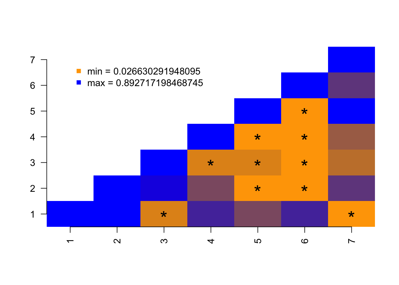

This function can also be used as a binary display when running a series of pairwise t-tests. For example, the following script runs a wilcoxon test between the time-slices from the disparity example dataset and displays in black which pairs of slices have a p-value below 0.05:

## Loading disparity data
data(disparity)

## Testing the pairwise difference between slices
tests <- test.dispRity(disparity, test = wilcox.test, correction = "bonferroni")

## Plotting the significance
pair.plot(as.data.frame(tests), what = "p.value", binary = 0.05)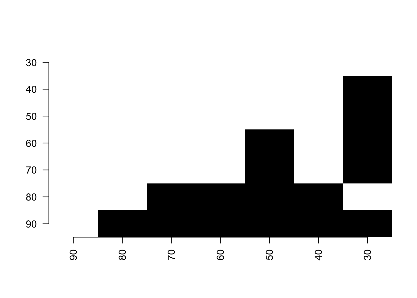

6.5 reduce.matrix

This function allows to reduce columns or rows of a matrix to make sure that there is enough overlap for further analysis. This is particularly useful if you are going to use distance matrices since it uses the vegan::vegdist function to test whether distances can be calculated or not.

For example, if we have a patchy matrix like so (where the black squares represent available data):

set.seed(1)
## A 10*5 matrix
na_matrix <- matrix(rnorm(50), 10, 5)
## Making sure some rows don't overlap
na_matrix[1, 1:2] <- NA
na_matrix[2, 3:5] <- NA
## Adding 50% NAs
na_matrix[sample(1:50, 25)] <- NA
## Illustrating the gappy matrix
image(t(na_matrix), col = "black")

We can use the reduce.matrix to double check whether any rows cannot be compared. The functions needs as an input the type of distance that will be used, say a "gower" distance:

## Reducing the matrix by row
(reduction <- reduce.matrix(na_matrix, distance = "gower"))

## $rows.to.remove
## [1] "9" "1"
## 
## $cols.to.remove
## NULL

We can not remove the rows 1 and 9 and see if that improved the overlap:

image(t(na_matrix[-as.numeric(reduction$rows.to.remove), ]), col = "black")

6.6 slice.tree

This function is a modification of the paleotree::timeSliceTree function that allows to make slices through a phylogenetic tree. Compared to the paleotree::timeSliceTree, this function allows a model to decide which tip or node to use when slicing through a branch (whereas paleotree::timeSliceTree always choose the first available tip alphabetically). The models for choosing which tip or node are the same as the ones used in the chrono.subsets and are described in chapter 03: specific tutorials.

The function works by using at least a tree, a slice age and a model:

set.seed(1)
## Generate a random ultrametric tree
tree <- rcoal(20)
## Add some node labels
tree$node.label <- letters[1:19]
## Add its root time
tree$root.time <- max(tree.age(tree)$ages)

## Slicing the tree at age 0.75
tree_75 <- slice.tree(tree, age = 0.75, "acctran")

## Showing both trees
par(mfrow = c(1,2))
plot(tree, main = "original tree")
axisPhylo() ; nodelabels(tree$node.label, cex = 0.8)
abline(v = (max(tree.age(tree)$ages) - 0.75), col = "red")
plot(tree_75, main = "sliced tree")

6.7 slide.nodes and remove.zero.brlen

This function allows to slide nodes along a tree! In other words it allows to change the branch length leading to a node without modifying the overall tree shape. This can be useful to add some value to 0 branch lengths for example.

The function works by taking a node (or a list of nodes), a tree and a sliding value. The node will be moved “up” (towards the tips) for the given sliding value. You can move the node “down” (towards the roots) using a negative value.

set.seed(42)
## Generating simple coalescent tree
tree <- rcoal(5)

## Sliding node 8 up and down
tree_slide_up <- slide.nodes(8, tree, slide = 0.075)
tree_slide_down <- slide.nodes(8, tree, slide = -0.075)

## Display the results
par(mfrow = c(3,1))
plot(tree, main = "original tree") ; axisPhylo() ; nodelabels()
plot(tree_slide_up, main = "slide up!") ; axisPhylo() ; nodelabels()
plot(tree_slide_down, main = "slide down!") ; axisPhylo() ; nodelabels()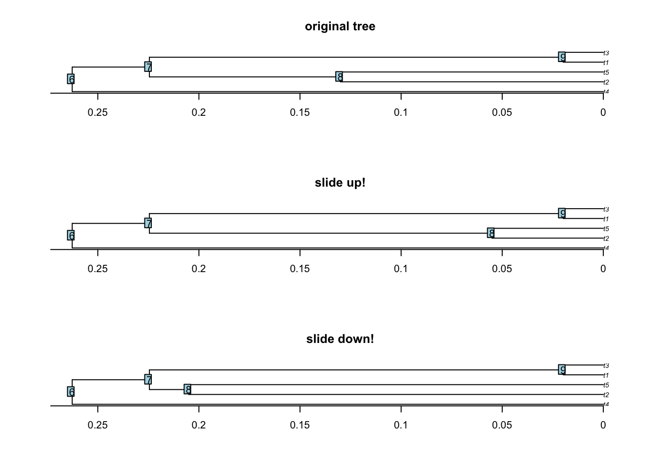

The remove.zero.brlen is a “clever” wrapping function that uses the slide.nodes function to stochastically remove zero branch lengths across a whole tree. This function will slide nodes up or down in successive postorder traversals (i.e. going down the tree clade by clade) in order to minimise the number of nodes to slide while making sure there are no silly negative branch lengths produced! By default it is trying to slide the nodes using 1% of the minimum branch length to avoid changing the topology too much.

set.seed(42)
## Generating a tree
tree <- rtree(20)

## Adding some zero branch lengths (5)
tree$edge.length[sample(1:Nedge(tree), 5)] <- 0

## And now removing these zero branch lengths!
tree_no_zero <- remove.zero.brlen(tree)

## Exaggerating the removal (to make it visible)
tree_exaggerated <- remove.zero.brlen(tree, slide = 1)

## Check the differences
any(tree$edge.length == 0)

## [1] TRUE

any(tree_no_zero$edge.length == 0)

## [1] FALSE

any(tree_exaggerated$edge.length == 0)

## [1] FALSE

## Display the results
par(mfrow = c(3,1))
plot(tree, main = "with zero edges")
plot(tree_no_zero, main = "without zero edges!")
plot(tree_exaggerated, main = "with longer edges")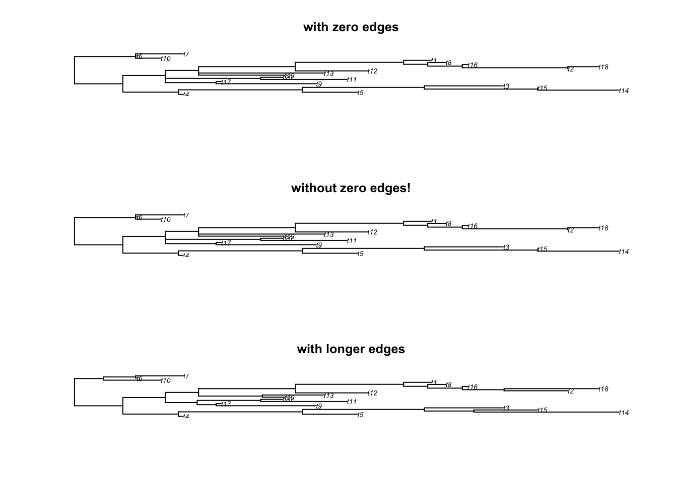

6.8 tree.age

This function allows to quickly calculate the ages of each tips and nodes present in a tree.

set.seed(1)
tree <- rtree(10)
## The tree age from a 10 tip tree
tree.age(tree)

##     ages elements
## 1  0.707       t7
## 2  0.142       t2
## 3  0.000       t3
## 4  1.467       t8
## 5  1.366       t1
## 6  1.895       t5
## 7  1.536       t6
## 8  1.456       t9
## 9  0.815      t10
## 10 2.343       t4
## 11 3.011       11
## 12 2.631       12
## 13 1.854       13
## 14 0.919       14
## 15 0.267       15
## 16 2.618       16
## 17 2.235       17
## 18 2.136       18
## 19 1.642       19

It also allows to set the age of the root of the tree:

## The ages starting from -100 units
tree.age(tree, age = 100)

##       ages elements
## 1   23.472       t7
## 2    4.705       t2
## 3    0.000       t3
## 4   48.736       t8
## 5   45.352       t1
## 6   62.931       t5
## 7   51.012       t6
## 8   48.349       t9
## 9   27.055      t10
## 10  77.800       t4
## 11 100.000       11
## 12  87.379       12
## 13  61.559       13
## 14  30.517       14
## 15   8.875       15
## 16  86.934       16
## 17  74.235       17
## 18  70.924       18
## 19  54.533       19

Usually tree age is calculated from the present to the past (e.g. in million years ago) but it is possible to reverse it using the order = present option:

## The ages in terms of tip/node height
tree.age(tree, order = "present")

##     ages elements
## 1  2.304       t7
## 2  2.869       t2
## 3  3.011       t3
## 4  1.544       t8
## 5  1.646       t1
## 6  1.116       t5
## 7  1.475       t6
## 8  1.555       t9
## 9  2.196      t10
## 10 0.668       t4
## 11 0.000       11
## 12 0.380       12
## 13 1.157       13
## 14 2.092       14
## 15 2.744       15
## 16 0.393       16
## 17 0.776       17
## 18 0.876       18
## 19 1.369       19