Phenotype Analysis of Brazilian Drought Trials

Last updated: 2025-01-13

Checks: 6 1

Knit directory: Genomic-Selection-for-Drought-Tolerance-Using-Genome-Wide-SNPs-in-Casava/

This reproducible R Markdown analysis was created with workflowr (version 1.7.1). The Checks tab describes the reproducibility checks that were applied when the results were created. The Past versions tab lists the development history.

R Markdown file: uncommitted changes

The R Markdown file has unstaged changes. To know which version of the R Markdown file created these results, you’ll want to first commit it to the Git repo. If you’re still working on the analysis, you can ignore this warning. When you’re finished, you can run wflow_publish to commit the R Markdown file and build the HTML.

Environment: empty

Great job! The global environment was empty. Objects defined in the global environment can affect the analysis in your R Markdown file in unknown ways. For reproduciblity it’s best to always run the code in an empty environment.

Seed: set.seed(20221020)

The command set.seed(20221020) was run prior to running the code in the R Markdown file. Setting a seed ensures that any results that rely on randomness, e.g. subsampling or permutations, are reproducible.

Session information: recorded

Great job! Recording the operating system, R version, and package versions is critical for reproducibility.

Cache: none

Nice! There were no cached chunks for this analysis, so you can be confident that you successfully produced the results during this run.

File paths: relative

Great job! Using relative paths to the files within your workflowr project makes it easier to run your code on other machines.

Repository version: 78cd01a

Great! You are using Git for version control. Tracking code development and connecting the code version to the results is critical for reproducibility.

The results in this page were generated with repository version 78cd01a. See the Past versions tab to see a history of the changes made to the R Markdown and HTML files.

Note that you need to be careful to ensure that all relevant files for the analysis have been committed to Git prior to generating the results (you can use wflow_publish or wflow_git_commit). workflowr only checks the R Markdown file, but you know if there are other scripts or data files that it depends on. Below is the status of the Git repository when the results were generated:


Ignored files:
    Ignored:    .Rhistory
    Ignored:    .Rproj.user/
    Ignored:    data/allchrAR08.txt

Untracked files:
    Untracked:  data/Articles/
    Untracked:  data/Artigo/
    Untracked:  data/Phenotyping2.xlsx
    Untracked:  data/dados__temp_umi.csv
    Untracked:  data/data.rar

Unstaged changes:
    Modified:   Genomic-Selection-for-Drought-Tolerance-Using-Genome-Wide-SNPs-in-Casava.Rproj
    Modified:   analysis/GWS.Rmd
    Modified:   analysis/mixed_models.Rmd
    Modified:   analysis/phenotype.Rmd
    Modified:   data/SNPs.rds
    Modified:   data/pheno_clean.csv
    Deleted:    output/BLUPS.csv
    Deleted:    output/BLUPS_par.Rdata
    Deleted:    output/README.md
    Deleted:    output/media_pheno.csv
    Deleted:    output/varcomp.csv

Note that any generated files, e.g. HTML, png, CSS, etc., are not included in this status report because it is ok for generated content to have uncommitted changes.

These are the previous versions of the repository in which changes were made to the R Markdown (analysis/phenotype.Rmd) and HTML (docs/phenotype.html) files. If you’ve configured a remote Git repository (see ?wflow_git_remote), click on the hyperlinks in the table below to view the files as they were in that past version.

File	Version	Author	Date	Message
html	21def57	WevertonGomesCosta	2025-01-13	update index and phenotype.html
Rmd	7b8bd72	WevertonGomesCosta	2025-01-13	update phenotype.Rmd
Rmd	77e21a6	Weverton Gomes	2025-01-13	Update Index and phenotype
html	97fd0b9	Weverton Gomes	2025-01-07	update about.html, license.html, phenotype.html
Rmd	54c6e28	Weverton Gomes	2025-01-07	update site, index.rmd, license.rmd, phenotype.rmd
html	c64a991	Weverton Gomes	2023-10-27	add phenotype html
Rmd	286b492	Weverton Gomes	2023-10-27	Update Scripts and README
Rmd	90dc112	WevertonGomesCosta	2022-11-17	Update
Rmd	6cc4d23	WevertonGomesCosta	2022-11-17	Update
html	6cc4d23	WevertonGomesCosta	2022-11-17	Update
html	d930880	WevertonGomesCosta	2022-11-11	Update
Rmd	5988c27	WevertonGomesCosta	2022-11-11	Update
html	5988c27	WevertonGomesCosta	2022-11-11	Update
Rmd	bf7b1d3	WevertonGomesCosta	2022-11-11	Update
html	bf7b1d3	WevertonGomesCosta	2022-11-11	Update

Libraries

Load the necessary libraries:

library(kableExtra)
library(tidyverse)
#if (!require("BiocManager", quietly = TRUE))
#    install.packages("BiocManager")
#BiocManager::install("ComplexHeatmap")
require(ComplexHeatmap)
library(data.table)
library(readxl)
library(metan)
library(DataExplorer)
library(ggthemes)
library(GGally)
theme_set(theme_bw())

Data import and manipulation

Import the phenotypic dataset, excluding traits without information and redundant traits:

pheno <- read_excel("data/Phenotyping2.xlsx", na = "NA") %>%
  select_if(~ !all(is.na(.))) %>%  # Deleting traits without information
  select(-c("Local", "Tratamento"))

Convert character traits to factors, and numeric grades to integer factors:

pheno <- pheno %>%
  mutate(across(c(Clone, Ano, row, col, Bloco), as.factor))

Exploratory Data Analysis

Provide an introductory analysis of the dataset:

introduce(pheno) %>%
  t() %>%
  kbl(escape = F, align = 'c') %>%
  kable_classic("hover", full_width = F, position = "center", fixed_thead = T)

rows	2336
columns	29
discrete_columns	6
continuous_columns	23
all_missing_columns	0
total_missing_values	16875
complete_rows	440
total_observations	67744
memory_usage	534240

We don’t have any columns that have all of the missing observations, but we do have a lot of missing values in every dataset. Some manipulations should be performed to improve the quality of the data.

Environment Analysis

Heatmap visualization of clone presence per year:

pheno_year_count <- pheno %>%
  count(Ano, Clone)

genmat <- model.matrix(~ -1 + Clone, data = pheno_year_count)
envmat <- model.matrix(~ -1 + Ano, data = pheno_year_count)
genenvmat <- t(envmat) %*% genmat
genenvmat_ch <- ifelse(genenvmat == 1, "Present", "Absent")

Heatmap(genenvmat_ch, 
        col = c("white", "tomato"), 
        show_column_names = F, 
        heatmap_legend_param = list(title = ""),
        column_title = "Genotypes", 
        row_title = "Environments")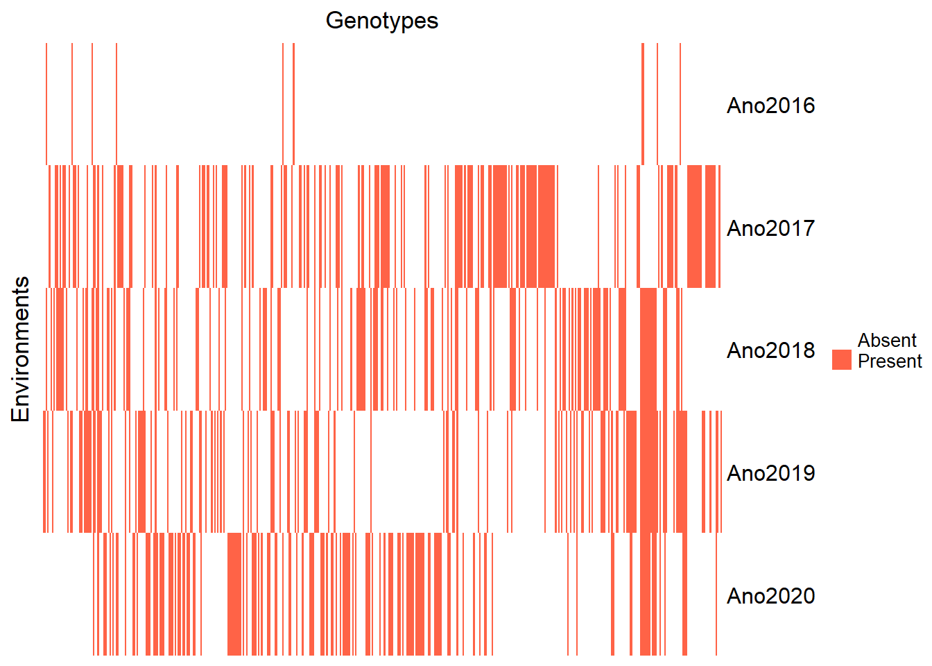

Version	Author	Date
77e21a6	Weverton Gomes	2025-01-13

Filter out the year 2016 due to insufficient observations:

pheno <- pheno %>%
  filter(Ano != 2016) %>%
  droplevels()

Reinspect the updated heatmap:

pheno_year_count <- pheno %>%
  count(Ano, Clone)

genmat <- model.matrix(~ -1 + Clone, data = pheno_year_count)
envmat <- model.matrix(~ -1 + Ano, data = pheno_year_count)
genenvmat <- t(envmat) %*% genmat
genenvmat_ch <- ifelse(genenvmat == 1, "Present", "Absent")

Heatmap(genenvmat_ch, 
        col = c("white", "tomato"), 
        show_column_names = F, 
        heatmap_legend_param = list(title = ""),
        column_title = "Genotypes", 
        row_title = "Environments")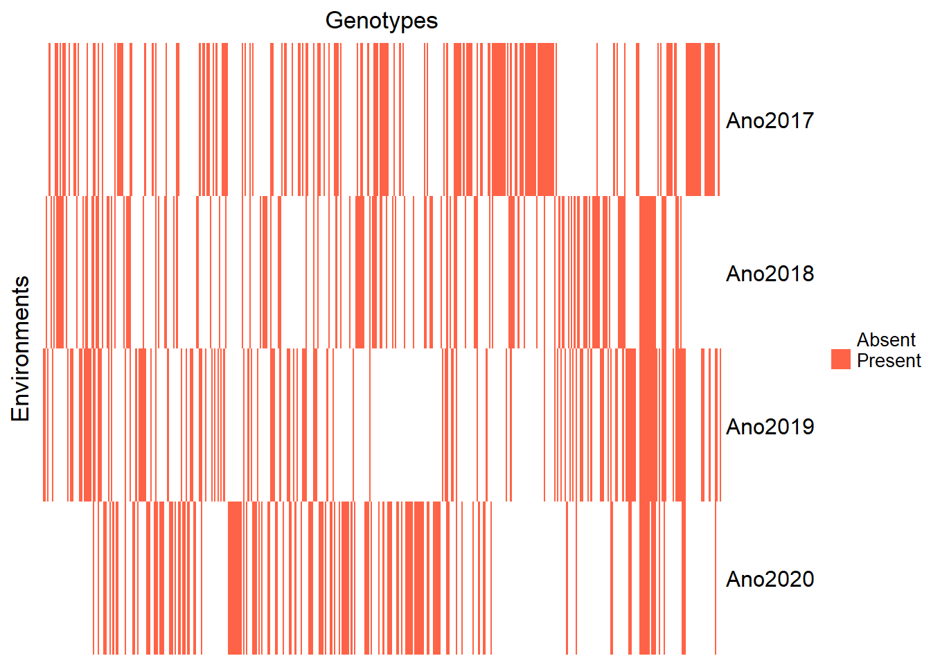

Version	Author	Date
77e21a6	Weverton Gomes	2025-01-13

Visualize the number of environments and genotypes:

genotype_year_table <- genenvmat %*% t(genenvmat) %>%
  kbl(escape = F, align = 'c') %>%
  kable_classic("hover", full_width = F, position = "center", fixed_thead = T)
rm(pheno_year_count, genmat, envmat, genenvmat, genenvmat_ch)
genotype_year_table

	Ano2017	Ano2018	Ano2019	Ano2020
Ano2017	165	42	22	14
Ano2018	42	138	39	16
Ano2019	22	39	133	29
Ano2020	14	16	29	138

Observe that some clones were evaluated in only one year. The number of clones evaluated across different years is summarized below:

pheno %>%
  count(Ano, Clone) %>%
  count(Clone) %>%
  count(n) %>%
  kbl(escape = F, align = 'c', col.names = c("N of Environment", "N of Genotypes")) %>%
  kable_classic("hover", full_width = F, position = "center", fixed_thead = T)

Storing counts in `nn`, as `n` already present in input
ℹ Use `name = "new_name"` to pick a new name.

N of Environment	N of Genotypes
1	350
2	72
3	20
4	5

Only 5 clones were evaluated in all years, which might affect the model’s accuracy. Therefore, adopting mixed models via REML in the analysis is suitable for obtaining BLUPs.

Analysis of traits

Provide descriptive statistics for each trait:

summary_table <- summary(pheno) %>%
  t() %>%
  kbl(escape = F, align = 'c') %>%
  kable_classic("hover", full_width = F, position = "center", fixed_thead = T)
summary_table


Clone	BGM-0164: 16	BGM-0170: 16	BGM-0396: 16	BGM-1243: 16	BGM-1267: 16	BGM-0134: 12	(Other) :2204
Ano	2017:660	2018:552	2019:532	2020:552	NA	NA	NA
Bloco	1:574	2:574	3:574	4:574	NA	NA	NA
row	11 : 121	3 : 120	10 : 120	2 : 119	6 : 118	4 : 117	(Other):1581
col	6 : 131	4 : 130	8 : 130	2 : 128	5 : 128	9 : 128	(Other):1521
N_Roots	Min. : 0.125	1st Qu.: 2.333	Median : 4.000	Mean : 4.293	3rd Qu.: 6.000	Max. :15.667	NA’s :322
FRY	Min. : 0.116	1st Qu.: 1.857	Median : 3.750	Mean : 4.946	3rd Qu.: 6.857	Max. :22.200	NA’s :335
ShY	Min. : 0.694	1st Qu.: 6.944	Median :11.167	Mean :14.228	3rd Qu.:18.714	Max. :61.167	NA’s :211
DMC	Min. :11.98	1st Qu.:25.00	Median :28.80	Mean :29.06	3rd Qu.:32.78	Max. :48.34	NA’s :968
StY	Min. :0.0154	1st Qu.:0.5494	Median :1.2068	Mean :1.5164	3rd Qu.:2.1092	Max. :8.8669	NA’s :978
Plant.Height	Min. :0.3600	1st Qu.:0.9633	Median :1.1600	Mean :1.1919	3rd Qu.:1.3908	Max. :3.0333	NA’s :220
HI	Min. : 1.574	1st Qu.:15.726	Median :23.345	Mean :24.556	3rd Qu.:31.884	Max. :71.967	NA’s :341
StC	Min. : 7.326	1st Qu.:20.350	Median :24.147	Mean :24.419	3rd Qu.:28.160	Max. :43.686	NA’s :968
PltArc	Min. :1.000	1st Qu.:1.000	Median :2.000	Mean :1.996	3rd Qu.:3.000	Max. :5.000	NA’s :678
Leaf.Ret	Min. :0.3333	1st Qu.:1.0000	Median :1.3333	Mean :1.7796	3rd Qu.:2.0000	Max. :5.0000	NA’s :216
Root.Le	Min. : 7.00	1st Qu.:19.00	Median :23.00	Mean :23.21	3rd Qu.:27.00	Max. :47.33	NA’s :339
Root.Di	Min. : 6.12	1st Qu.:23.36	Median :28.17	Mean :28.88	3rd Qu.:33.50	Max. :63.30	NA’s :339
Stem.D	Min. :1.013	1st Qu.:1.859	Median :2.101	Mean :2.112	3rd Qu.:2.362	Max. :4.373	NA’s :224
Mite	Min. :1.000	1st Qu.:3.000	Median :3.667	Mean :3.475	3rd Qu.:4.000	Max. :5.000	NA’s :222
Incidence_Mites	Min. :1	1st Qu.:1	Median :1	Mean :1	3rd Qu.:1	Max. :1	NA’s :674
Nstem.Plant	Min. :1.000	1st Qu.:1.333	Median :2.000	Mean :2.131	3rd Qu.:2.667	Max. :6.667	NA’s :850
Stand6MAP	Min. :1.000	1st Qu.:4.000	Median :6.000	Mean :5.202	3rd Qu.:7.000	Max. :8.000	NA’s :849
Branching	Min. :0.0000	1st Qu.:0.0000	Median :0.3333	Mean :0.5911	3rd Qu.:1.0000	Max. :4.0000	NA’s :673
Staygreen	Min. :1.000	1st Qu.:1.000	Median :1.000	Mean :1.292	3rd Qu.:2.000	Max. :3.000	NA’s :669
Vigor	Mode:logical	TRUE:1075	NA’s:1221	NA	NA	NA	NA
Flowering	Min. :0.0000	1st Qu.:0.0000	Median :0.0000	Mean :0.0074	3rd Qu.:0.0000	Max. :1.0000	NA’s :673
Canopy_Lenght	Min. : 10.00	1st Qu.: 54.33	Median : 72.00	Mean : 73.35	3rd Qu.: 91.67	Max. :240.17	NA’s :1458
Canopy_Width	Min. : 7.50	1st Qu.: 56.33	Median : 75.58	Mean : 76.68	3rd Qu.: 96.00	Max. :213.33	NA’s :1458
Leaf_Lenght	Min. : 3.750	1st Qu.: 8.417	Median :11.250	Mean :11.676	3rd Qu.:14.200	Max. :32.667	NA’s :1459

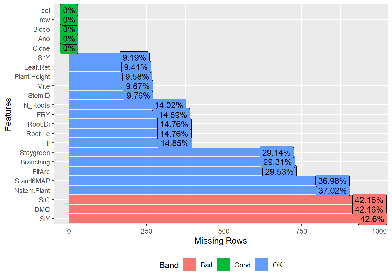
Exclude traits with high missing value ratios:

pheno <- pheno %>%
  select(-c(Incidence_Mites, Vigor, Flowering, Leaf_Lenght, Canopy_Width, Canopy_Lenght))

Ensure that the traits have acceptable missing value ratios:

plot_missing(pheno)

Version	Author	Date
77e21a6	Weverton Gomes	2025-01-13

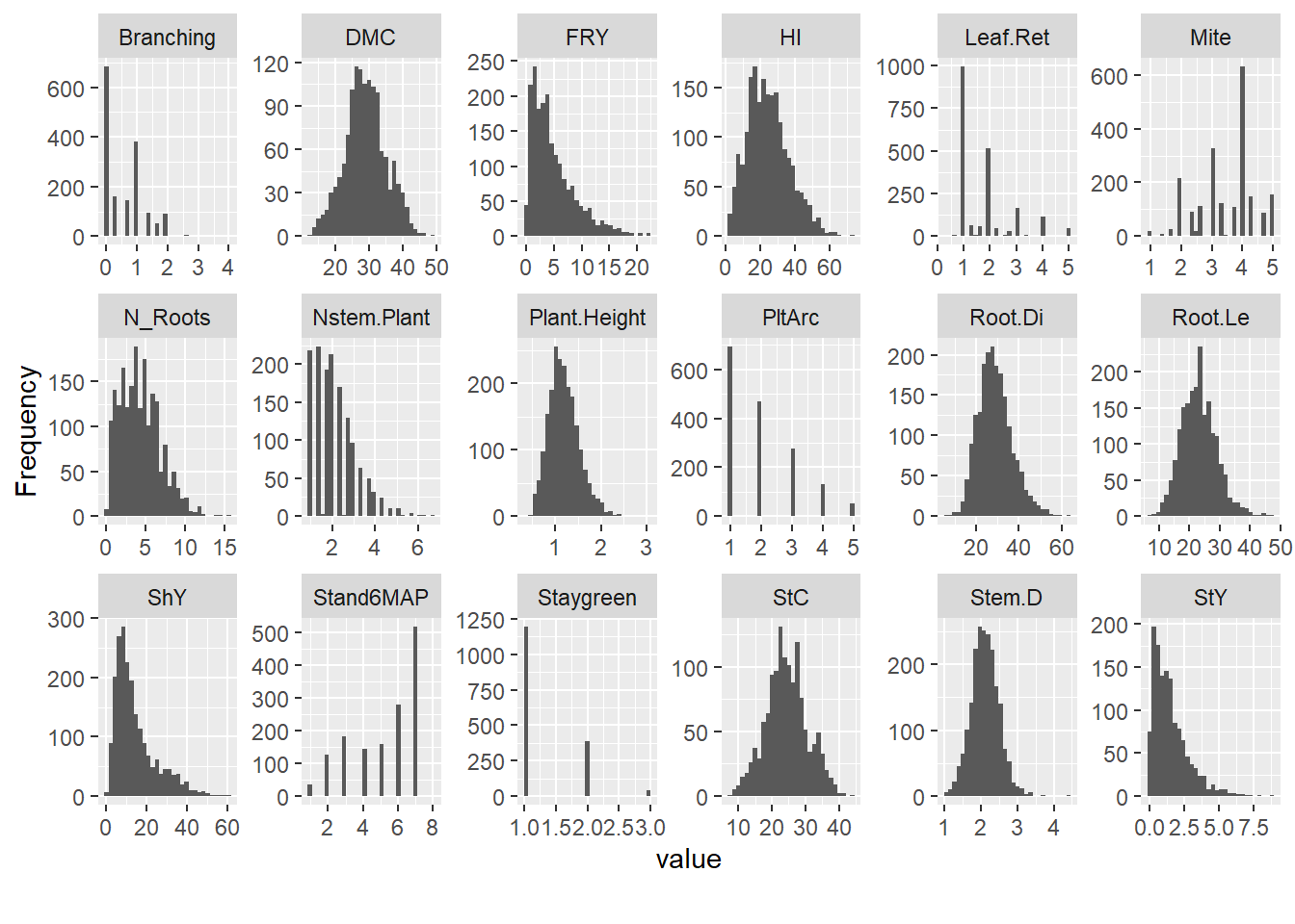
Evaluate the distribution of traits by year with histograms for quantitative traits:

plot_histogram(pheno, ncol = 6)

Version	Author	Date
77e21a6	Weverton Gomes	2025-01-13

Remove traits that lack normal distribution:

pheno <- pheno %>%
  select(-c(Branching, Leaf.Ret, Mite, PltArc, Stand6MAP, Staygreen))

Analisys of Clone

Inspect missing values by clone and year:

pheno_missing_summary <- pheno %>%
  select(-Bloco, -row, -col) %>%
  group_by(Clone, Ano) %>%
  summarise_all(.funs = list(~ sum(is.na(.)))) %>%
  ungroup() %>%
  select_numeric_cols() %>%
  mutate(mean = rowMeans(.),
         Clone.Ano = factor(unique(interaction(pheno$Clone, pheno$Ano)))) %>%
  filter(mean > 2) %>%
  droplevels()

missing_genotypes <- nlevels(pheno_missing_summary$Clone.Ano) %>%
  kbl(escape = F, align = 'c', col.names = c("N of genotypes")) %>%
  kable_classic("hover", full_width = F, position = "center", fixed_thead = T)
missing_genotypes

N of genotypes
54

Evaluate clone and year descriptive statistics:

clone_year_stats <- ge_details(pheno, Ano, Clone, resp = everything()) %>%
  t() %>%
  kbl(escape = F, align = 'c') %>%
  kable_classic("hover", full_width = F, position = "center", fixed_thead = T)
clone_year_stats

Parameters	Mean	SE	SD	CV	Min	Max	MinENV	MaxENV	MinGEN	MaxGEN
N_Roots	4.29	0.06	2.51	58.56	0.12 (BGM-1031 in 2017)	15.67 (2012-107-002 in 2019)	2018 (1.62)	2019 (5.76)	BGM-0411 (0.33)	2012-107-002 (11.33)
FRY	4.95	0.09	4.04	81.79	0.12 (BGM-0886 in 2017)	22.2 (BGM-1267 in 2018)	2017 (2.75)	2020 (6.52)	BGM-1488 (0.34)	IAC-14 (14.07)
ShY	14.23	0.22	10.16	71.45	0.69 (BGM-0996 in 2017)	61.17 (BGM-2124 in 2020)	2017 (8.47)	2020 (25.87)	BGM-0048 (1.52)	BGM-2124 (54.33)
DMC	29.06	0.17	6.1	21	11.98 (BGM-0626 in 2020)	48.34 (BGM-1015 in 2020)	2020 (26.21)	2018 (35.38)	BGM-0626 (14.98)	BGM-1015 (45.02)
StY	1.52	0.04	1.27	84.01	0.02 (BGM-0340 in 2019)	8.87 (BGM-0396 in 2018)	2019 (1.32)	2018 (1.84)	BGM-0089 (0.06)	BGM-1023 (4.76)
Plant.Height	1.19	0.01	0.33	27.43	0.36 (BGM-0426 in 2020)	3.03 (BR-11-24-156 in 2020)	2017 (1)	2019 (1.48)	Jatobá (0.58)	BGM-1200 (1.91)
HI	24.56	0.27	11.89	48.42	1.57 (BGM-1159 in 2017)	71.97 (BGM-1315 in 2018)	2020 (18.61)	2018 (32.36)	BGM-0961 (2.5)	Mata_Fome_Branca (52.78)
StC	24.42	0.17	6.11	25.05	7.33 (BGM-0626 in 2020)	43.69 (BGM-1015 in 2020)	2020 (21.56)	2018 (30.78)	BGM-0626 (10.33)	BGM-1015 (40.37)
Root.Le	23.21	0.13	5.8	24.99	7 (BGM-1574 in 2017)	47.33 (BGM-0396 in 2018)	2017 (19.72)	2019 (27.14)	Jatobá (8.5)	BGM-1956 (35.5)
Root.Di	28.88	0.18	7.9	27.35	6.12 (BGM-2142 in 2019)	63.3 (BRS Mulatinha in 2018)	2017 (24.49)	2018 (34.74)	BGM-0089 (12.14)	BGM-1956 (48.91)
Stem.D	2.11	0.01	0.38	17.9	1.01 (BGM-0592 in 2018)	4.37 (BRS Tapioqueira in 2020)	2018 (2.02)	2017 (2.16)	BGM-0048 (1.25)	BGM-1523 (2.93)
Nstem.Plant	2.13	0.03	0.95	44.53	1 (BGM-0036 in 2018)	6.67 (BGM-0714 in 2019)	2018 (1.44)	2019 (2.71)	BGM-0066 (1)	BGM-0451 (4.44)

Again, some traits were not computed for the year 2017, so we have to eliminate that year when performing the analysis for these traits.

Evaluate the clone-only descriptive statistics for the traits.

cv_stats <- desc_stat(pheno, by = Ano, na.rm = TRUE, stats = "cv") %>%
  na.omit() %>%
  arrange(desc(cv)) %>%
  pivot_wider(names_from = "Ano", values_from = "cv") %>%
  kbl(escape = F, align = 'c') %>%
  kable_classic("hover", full_width = F, position = "center", fixed_thead = T)
cv_stats

variable	2018	2020	2019	2017
StY	91.8742	81.2220	72.3243	NA
FRY	86.0073	68.4455	70.0326	66.8379
ShY	69.0625	42.7475	47.4901	45.4973
N_Roots	63.2913	47.0839	47.2357	48.8708
HI	41.5442	43.3204	41.8572	48.2942
Nstem.Plant	33.3849	37.1507	37.3740	NA
Plant.Height	28.0409	24.0927	19.1125	21.0398
StC	15.6937	27.3600	16.5407	NA
Root.Le	27.1625	18.9730	21.1089	21.5823
Root.Di	23.3943	20.5858	24.3155	21.0039
DMC	13.6086	22.5059	13.8212	NA
Stem.D	22.3941	17.5042	15.7037	16.7774

Some traits were not computed for the year 2017, so we have to eliminate that year when performing the analysis for these traits and some traits presented hight cv, as StY and FRY.

General Inspection

Identifying outliers in all non-categorical variables:

inspect(pheno %>%
          select_if(~ !is.factor(.)), verbose = FALSE) %>%
  arrange(desc(Outlier)) %>%
  kbl(escape = F, align = 'c') %>%
  kable_classic(
    "hover",
    full_width = F,
    position = "center",
    fixed_thead = T
  )

Variable	Class	Missing	Valid_n	Min	Median	Max	Outlier	Text
ShY	numeric	Yes	2085	0.69	11.17	61.17	89	NA
FRY	numeric	Yes	1961	0.12	3.75	22.20	71	NA
StY	numeric	Yes	1318	0.02	1.21	8.87	49	NA
Root.Di	numeric	Yes	1957	6.12	28.17	63.30	32	NA
Nstem.Plant	numeric	Yes	1446	1.00	2.00	6.67	30	NA
Plant.Height	numeric	Yes	2076	0.36	1.16	3.03	23	NA
Stem.D	numeric	Yes	2072	1.01	2.10	4.37	22	NA
Root.Le	numeric	Yes	1957	7.00	23.00	47.33	19	NA
N_Roots	numeric	Yes	1974	0.12	4.00	15.67	16	NA
HI	numeric	Yes	1955	1.57	23.35	71.97	15	NA
DMC	numeric	Yes	1328	11.98	28.80	48.34	6	NA
StC	numeric	Yes	1328	7.33	24.15	43.69	6	NA

Confirming what was previously described, most traits with high coefficients of variation (CV) have many outliers.

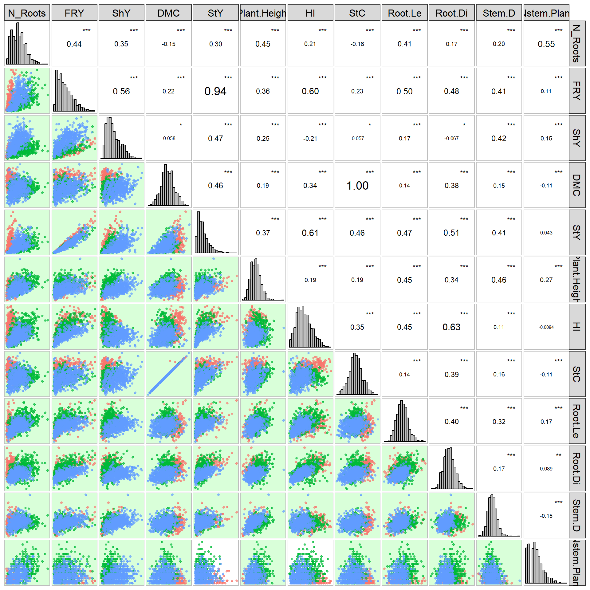
Inspect overall data correlations and save clean data:

# Plotting correlations
corr_plot(pheno, col.by = Ano)

Version	Author	Date
0d2a1ed	WevertonGomesCosta	2025-01-13
77e21a6	Weverton Gomes	2025-01-13

Climate data

# Load the climate data
climate_data <- read.csv("data/dados__temp_umi.csv", sep = ";", na = "null", dec = ",")

# Convert the date column to date format
climate_data$Data.Medicao <- dmy(climate_data$Data.Medicao)

# Extract the year and semester from the date
climate_data <- climate_data %>%
  mutate(Ano = year(Data.Medicao), Semestre = ifelse(month(Data.Medicao) <= 6, "1-6", "7-12"))

# Calculate the means per semester and year for each variable
semester_means <- climate_data %>%
  group_by(Ano, Semestre) %>%
  summarise_if(is.numeric, ~mean(., na.rm = TRUE))

# Display the results
semester_means %>%
  kbl(escape = F, align = 'c') %>%
  kable_classic("hover", full_width = F, position = "center", fixed_thead = T)

Ano	Semestre	EVAPORACAO.DO.PICHE..DIARIA.mm.	INSOLACAO.TOTAL..DIARIO.h.	PRECIPITACAO.TOTAL..DIARIO.mm.	TEMPERATURA.MAXIMA..DIARIA..C.	TEMPERATURA.MEDIA.COMPENSADA..DIARIA..C.	TEMPERATURA.MINIMA..DIARIA..C.	UMIDADE.RELATIVA.DO.AR..MEDIA.DIARIA…	UMIDADE.RELATIVA.DO.AR..MINIMA.DIARIA…	VENTO..VELOCIDADE.MEDIA.DIARIA.m.s.
2016	1-6	10.607182	8.453297	1.7829670	32.94780	27.85220	23.30440	65.63571	55.33516	2.703846
2016	7-12	13.772826	9.549456	0.1625000	33.72609	28.05217	22.64511	58.46141	47.90217	3.155978
2017	1-6	12.409945	8.513260	0.5801105	33.51271	28.48122	23.77845	60.43833	50.20994	2.971271
2017	7-12	13.032065	8.686957	0.2304348	32.30109	26.99239	22.08533	55.83770	44.88587	3.279891
2018	1-6	9.982873	7.917680	1.4602210	32.39779	27.39116	23.11713	62.37821	50.77348	2.782320
2018	7-12	12.984239	9.203261	0.3222826	33.13152	27.72283	22.60054	54.03859	43.55978	3.023913
2019	1-6	10.839326	8.501695	1.1387640	33.57175	28.31243	23.88596	61.06723	48.66298	2.758989
2019	7-12	13.895652	9.229891	0.1972826	33.72391	27.91413	22.59565	53.56667	43.01087	3.244565
2020	1-6	8.186517	6.869101	1.9252809	32.20337	27.24157	23.48090	70.01461	59.37234	2.555056
2020	7-12	12.382065	8.848913	0.9619565	32.79946	27.07017	21.95217	59.94088	47.12500	3.020109

Then, now we go to execute the mixed models analisys script: mixed_models.Rmd

sessionInfo()

R version 4.3.1 (2023-06-16 ucrt)
Platform: x86_64-w64-mingw32/x64 (64-bit)
Running under: Windows 10 x64 (build 19045)

Matrix products: default


locale:
[1] LC_COLLATE=Portuguese_Brazil.utf8  LC_CTYPE=Portuguese_Brazil.utf8   
[3] LC_MONETARY=Portuguese_Brazil.utf8 LC_NUMERIC=C                      
[5] LC_TIME=Portuguese_Brazil.utf8    

time zone: America/Sao_Paulo
tzcode source: internal

attached base packages:
[1] grid      stats     graphics  grDevices utils     datasets  methods  
[8] base     

other attached packages:
 [1] GGally_2.1.2          ggthemes_4.2.4        DataExplorer_0.8.2   
 [4] metan_1.18.0          readxl_1.4.3          data.table_1.14.8    
 [7] ComplexHeatmap_2.16.0 lubridate_1.9.2       forcats_1.0.0        
[10] stringr_1.5.0         dplyr_1.1.2           purrr_1.0.2          
[13] readr_2.1.4           tidyr_1.3.0           tibble_3.2.1         
[16] ggplot2_3.4.3         tidyverse_2.0.0       kableExtra_1.3.4     

loaded via a namespace (and not attached):
  [1] gridExtra_2.3       writexl_1.4.2       rlang_1.1.1        
  [4] magrittr_2.0.3      clue_0.3-64         GetoptLong_1.0.5   
  [7] git2r_0.32.0        matrixStats_1.0.0   compiler_4.3.1     
 [10] png_0.1-8           systemfonts_1.0.4   vctrs_0.6.3        
 [13] rvest_1.0.3         pkgconfig_2.0.3     shape_1.4.6        
 [16] crayon_1.5.2        fastmap_1.1.1       labeling_0.4.2     
 [19] utf8_1.2.3          promises_1.2.1      rmarkdown_2.24     
 [22] tzdb_0.4.0          nloptr_2.0.3        xfun_0.40          
 [25] cachem_1.0.8        jsonlite_1.8.7      highr_0.10         
 [28] later_1.3.1         reshape_0.8.9       tweenr_2.0.2       
 [31] parallel_4.3.1      cluster_2.1.4       R6_2.5.1           
 [34] bslib_0.5.1         stringi_1.7.12      RColorBrewer_1.1-3 
 [37] boot_1.3-28.1       numDeriv_2016.8-1.1 jquerylib_0.1.4    
 [40] cellranger_1.1.0    Rcpp_1.0.11         iterators_1.0.14   
 [43] knitr_1.43          IRanges_2.34.1      igraph_1.5.1       
 [46] Matrix_1.6-1        httpuv_1.6.11       splines_4.3.1      
 [49] timechange_0.2.0    tidyselect_1.2.0    rstudioapi_0.15.0  
 [52] yaml_2.3.7          doParallel_1.0.17   codetools_0.2-19   
 [55] lmerTest_3.1-3      lattice_0.21-8      plyr_1.8.8         
 [58] withr_2.5.2         evaluate_0.22       polyclip_1.10-4    
 [61] xml2_1.3.5          circlize_0.4.15     pillar_1.9.0       
 [64] whisker_0.4.1       foreach_1.5.2       stats4_4.3.1       
 [67] generics_0.1.3      rprojroot_2.0.3     mathjaxr_1.6-0     
 [70] S4Vectors_0.38.1    hms_1.1.3           munsell_0.5.0      
 [73] scales_1.2.1        minqa_1.2.6         glue_1.6.2         
 [76] tools_4.3.1         lme4_1.1-34         webshot_0.5.5      
 [79] fs_1.6.3            colorspace_2.1-0    networkD3_0.4      
 [82] nlme_3.1-163        patchwork_1.1.3     ggforce_0.4.1      
 [85] cli_3.6.1           workflowr_1.7.1     fansi_1.0.4        
 [88] viridisLite_0.4.2   svglite_2.1.1       gtable_0.3.4       
 [91] sass_0.4.7          digest_0.6.33       BiocGenerics_0.46.0
 [94] ggrepel_0.9.3       htmlwidgets_1.6.2   rjson_0.2.21       
 [97] farver_2.1.1        htmltools_0.5.6     lifecycle_1.0.3    
[100] httr_1.4.7          GlobalOptions_0.1.2 MASS_7.3-60

Weverton Gomes da Costa, Pós-Doutorando, Embrapa Mandioca e Fruticultura, wevertonufv@gmail.com ↩︎