Análise dos Componentes de Variância para 18 Modelos Preditivos

workflowr

• Summary
• Checks
• Past versions

Last updated: 2026-02-24

Checks: 6 1

Knit directory: Integrating-nir-genomic-kernel/

This reproducible R Markdown analysis was created with workflowr (version 1.7.2). The Checks tab describes the reproducibility checks that were applied when the results were created. The Past versions tab lists the development history.

---

R Markdown file: uncommitted changes

The R Markdown file has unstaged changes. To know which version of the R Markdown file created these results, you’ll want to first commit it to the Git repo. If you’re still working on the analysis, you can ignore this warning. When you’re finished, you can run wflow_publish to commit the R Markdown file and build the HTML.

Environment: empty

Great job! The global environment was empty. Objects defined in the global environment can affect the analysis in your R Markdown file in unknown ways. For reproduciblity it’s best to always run the code in an empty environment.

Seed: set.seed(20250829)

The command set.seed(20250829) was run prior to running the code in the R Markdown file. Setting a seed ensures that any results that rely on randomness, e.g. subsampling or permutations, are reproducible.

Session information: recorded

Great job! Recording the operating system, R version, and package versions is critical for reproducibility.

Cache: none

Nice! There were no cached chunks for this analysis, so you can be confident that you successfully produced the results during this run.

File paths: relative

Great job! Using relative paths to the files within your workflowr project makes it easier to run your code on other machines.

Repository version: c94fde8

Great! You are using Git for version control. Tracking code development and connecting the code version to the results is critical for reproducibility.

The results in this page were generated with repository version c94fde8. See the Past versions tab to see a history of the changes made to the R Markdown and HTML files.

Note that you need to be careful to ensure that all relevant files for the analysis have been committed to Git prior to generating the results (you can use wflow_publish or wflow_git_commit). workflowr only checks the R Markdown file, but you know if there are other scripts or data files that it depends on. Below is the status of the Git repository when the results were generated:

Ignored files:
    Ignored:    .Rhistory
    Ignored:    .Rproj.user/
    Ignored:    data/Article_documents/
    Ignored:    data/Maize-NIRS-GBS-main/
    Ignored:    output/Matrizes/ZEZE.rds
    Ignored:    output/adjust_models/
    Ignored:    output/climate_results/additional_climate_plots.tiff
    Ignored:    output/climate_results/combined_additional_climate_plots.tiff
    Ignored:    output/climate_results/combined_climate_plot.tiff
    Ignored:    output/cv-schemes.tiff
    Ignored:    output/variance_components/rep_1/
    Ignored:    output/variance_components/rep_10/
    Ignored:    output/variance_components/rep_11/
    Ignored:    output/variance_components/rep_12/
    Ignored:    output/variance_components/rep_13/
    Ignored:    output/variance_components/rep_14/
    Ignored:    output/variance_components/rep_15/
    Ignored:    output/variance_components/rep_16/
    Ignored:    output/variance_components/rep_17/
    Ignored:    output/variance_components/rep_18/
    Ignored:    output/variance_components/rep_19/
    Ignored:    output/variance_components/rep_2/
    Ignored:    output/variance_components/rep_20/
    Ignored:    output/variance_components/rep_3/
    Ignored:    output/variance_components/rep_4/
    Ignored:    output/variance_components/rep_5/
    Ignored:    output/variance_components/rep_6/
    Ignored:    output/variance_components/rep_7/
    Ignored:    output/variance_components/rep_8/
    Ignored:    output/variance_components/rep_9/
    Ignored:    output/variance_components/var_components_GY.tiff
    Ignored:    output/variance_components/var_components_KW.tiff
    Ignored:    output/variance_components/var_components_combined.tiff
    Ignored:    output/variance_components/variance_components_all.dat
    Ignored:    output/variance_components/variance_components_all.rds

Untracked files:
    Untracked:  output/variance_components/variance_components_processed.csv

Unstaged changes:
    Modified:   analysis/variance_components.Rmd
    Modified:   analysis/visualization.Rmd
    Deleted:    output/Pred.ability/Pred.ability.CV0.CS11_WS.csv
    Deleted:    output/Pred.ability/Pred.ability.CV0.CS11_WW.csv
    Deleted:    output/Pred.ability/Pred.ability.CV0.CS12_WS.csv
    Deleted:    output/Pred.ability/Pred.ability.CV0.CS12_WW.csv
    Deleted:    output/Pred.ability/Pred.ability.CV0.CV00.classified.csv
    Deleted:    output/Pred.ability/Pred.ability.CV0.CV00.csv
    Deleted:    output/Pred.ability/Pred.ability.CV0.CV00.filtered.csv
    Deleted:    output/Pred.ability/Pred.ability.CV00.CS11_WS.csv
    Deleted:    output/Pred.ability/Pred.ability.CV00.CS11_WW.csv
    Deleted:    output/Pred.ability/Pred.ability.CV00.CS12_WS.csv
    Deleted:    output/Pred.ability/Pred.ability.CV00.CS12_WW.csv
    Deleted:    output/Pred.ability/Pred.ability.CV1.CV2.classified.csv
    Deleted:    output/Pred.ability/Pred.ability.CV1.CV2.csv
    Deleted:    output/Pred.ability/Pred.ability.CV1.CV2.filtered.csv
    Deleted:    output/variance_components/Variance.Components.DAT.Means.csv
    Deleted:    output/variance_components/Variance.Components.Percentage.PlotData.csv

Note that any generated files, e.g. HTML, png, CSS, etc., are not included in this status report because it is ok for generated content to have uncommitted changes.

---

These are the previous versions of the repository in which changes were made to the R Markdown (analysis/variance_components.Rmd) and HTML (docs/variance_components.html) files. If you’ve configured a remote Git repository (see ?wflow_git_remote), click on the hyperlinks in the table below to view the files as they were in that past version.

File	Version	Author	Date	Message
Rmd	c996e1e	WevertonGomesCosta	2026-02-24	update
Rmd	5b10ff7	WevertonGomesCosta	2026-02-24	update
Rmd	1a46586	WevertonGomesCosta	2025-11-04	update variance_components .rmd and .html
html	1a46586	WevertonGomesCosta	2025-11-04	update variance_components .rmd and .html
Rmd	f18937a	WevertonGomesCosta	2025-11-04	chance components_variance to variance_components

---

Introdução

Este documento realiza a análise de componentes de variância para os 18 modelos preditivos definidos anteriormente. A partir das matrizes de parentesco (kernels), ajustamos cada modelo ao conjunto completo de dados para estimar a proporção da variância fenotípica atribuída a cada componente (genético, ambiental, interações, etc.). Essas estimativas ajudam a compreender a estrutura dos dados e a importância relativa dos diferentes kernels.

O script é dividido em duas partes principais:

1. Cálculo dos componentes de variância (execução paralela com BGLR) – gera o arquivo variance_components_raw.csv.
2. Processamento e visualização – carrega o arquivo bruto, calcula porcentagens e produz gráficos.

Caso você já tenha o arquivo variance_components_raw.csv, pode pular diretamente para a seção de processamento.

1. Carregar Pacotes e Matrizes

library(tidyverse)
library(BGLR)
library(parallel)
library(doParallel)
library(ggthemes)    # para paleta de cores
library(scales)      # para formatação de percentuais

source_dir <- "output/Matrizes/"

# Kernels lineares e ambientais
ZG    <- readRDS(paste0(source_dir, "ZG.rds"))
ZP    <- readRDS(paste0(source_dir, "ZP.rds"))
ZE    <- readRDS(paste0(source_dir, "ZE.rds"))
ZEZE  <- readRDS(paste0(source_dir, "ZEZE.rds"))
ZW    <- readRDS(paste0(source_dir, "ZW.rds"))

# Interações lineares
ZGZE  <- readRDS(paste0(source_dir, "ZGZE.rds"))
ZPZE  <- readRDS(paste0(source_dir, "ZPZE.rds"))
ZGZW  <- readRDS(paste0(source_dir, "ZGZW.rds"))
ZPZW  <- readRDS(paste0(source_dir, "ZPZW.rds"))

# Kernels não lineares
GGK   <- readRDS(paste0(source_dir, "GGK.rds"))
PGK   <- readRDS(paste0(source_dir, "PGK.rds"))
GAK   <- readRDS(paste0(source_dir, "GAK.rds"))
PAK   <- readRDS(paste0(source_dir, "PAK.rds"))

# Interações não lineares
GGKE  <- readRDS(paste0(source_dir, "GGKE.rds"))
PGKE  <- readRDS(paste0(source_dir, "PGKE.rds"))
GGKW  <- readRDS(paste0(source_dir, "GGKW.rds"))
PGKW  <- readRDS(paste0(source_dir, "PGKW.rds"))

GAKE  <- readRDS(paste0(source_dir, "GAKE.rds"))
PAKE  <- readRDS(paste0(source_dir, "PAKE.rds"))
GAKW  <- readRDS(paste0(source_dir, "GAKW.rds"))
PAKW  <- readRDS(paste0(source_dir, "PAKW.rds"))

# Dados fenotípicos e pedigree
Pheno    <- readRDS(paste0(source_dir, "Pheno.rds"))
Pedigree <- readRDS(paste0(source_dir, "Pedigree.rds"))

n_hybrids <- length(Pedigree)
cat("Número total de observações:", n_hybrids, "\n")

Número total de observações: 329 

2. Definição dos 18 Modelos

Cada modelo é uma lista no formato exigido pelo argumento ETA do BGLR. Os efeitos de ambiente (E) são tratados como fixos (model = "BRR"), enquanto os kernels são aleatórios (model = "RKHS").

modelos <- list()

# Modelo 1: E + G + GE
modelos[[1]] <- list(
  E  = list(X = ZE, model = "BRR"),
  G  = list(K = ZG, model = "RKHS"),
  GE = list(K = ZGZE, model = "RKHS")
)

# Modelo 2: E + P + PE
modelos[[2]] <- list(
  E  = list(X = ZE, model = "BRR"),
  P  = list(K = ZP, model = "RKHS"),
  PE = list(K = ZPZE, model = "RKHS")
)

# Modelo 3: E + GGK + GGKE
modelos[[3]] <- list(
  E    = list(X = ZE, model = "BRR"),
  GGK  = list(K = GGK, model = "RKHS"),
  GGKE = list(K = GGKE, model = "RKHS")
)

# Modelo 4: E + PGK + PGKE
modelos[[4]] <- list(
  E    = list(X = ZE, model = "BRR"),
  PGK  = list(K = PGK, model = "RKHS"),
  PGKE = list(K = PGKE, model = "RKHS")
)

# Modelo 5: E + GAK + GAKE
modelos[[5]] <- list(
  E    = list(X = ZE, model = "BRR"),
  GAK  = list(K = GAK, model = "RKHS"),
  GAKE = list(K = GAKE, model = "RKHS")
)

# Modelo 6: E + PAK + PAKE
modelos[[6]] <- list(
  E    = list(X = ZE, model = "BRR"),
  PAK  = list(K = PAK, model = "RKHS"),
  PAKE = list(K = PAKE, model = "RKHS")
)

# Modelo 7: E + G + P + GE + PE
modelos[[7]] <- list(
  E  = list(X = ZE, model = "BRR"),
  G  = list(K = ZG, model = "RKHS"),
  P  = list(K = ZP, model = "RKHS"),
  GE = list(K = ZGZE, model = "RKHS"),
  PE = list(K = ZPZE, model = "RKHS")
)

# Modelo 8: E + GGK + PGK + GGKE + PGKE
modelos[[8]] <- list(
  E    = list(X = ZE, model = "BRR"),
  GGK  = list(K = GGK, model = "RKHS"),
  PGK  = list(K = PGK, model = "RKHS"),
  GGKE = list(K = GGKE, model = "RKHS"),
  PGKE = list(K = PGKE, model = "RKHS")
)

# Modelo 9: E + GAK + PAK + GAKE + PAKE
modelos[[9]] <- list(
  E    = list(X = ZE, model = "BRR"),
  GAK  = list(K = GAK, model = "RKHS"),
  PAK  = list(K = PAK, model = "RKHS"),
  GAKE = list(K = GAKE, model = "RKHS"),
  PAKE = list(K = PAKE, model = "RKHS")
)

# Modelo 10: E + W + G + GE + GW
modelos[[10]] <- list(
  E  = list(X = ZE, model = "BRR"),
  W  = list(K = ZW, model = "RKHS"),
  G  = list(K = ZG, model = "RKHS"),
  GE = list(K = ZGZE, model = "RKHS"),
  GW = list(K = ZGZW, model = "RKHS")
)

# Modelo 11: E + W + P + PE + PW
modelos[[11]] <- list(
  E  = list(X = ZE, model = "BRR"),
  W  = list(K = ZW, model = "RKHS"),
  P  = list(K = ZP, model = "RKHS"),
  PE = list(K = ZPZE, model = "RKHS"),
  PW = list(K = ZPZW, model = "RKHS")
)

# Modelo 12: E + W + G + P + GE + PE + GW + PW
modelos[[12]] <- list(
  E  = list(X = ZE, model = "BRR"),
  W  = list(K = ZW, model = "RKHS"),
  G  = list(K = ZG, model = "RKHS"),
  P  = list(K = ZP, model = "RKHS"),
  GE = list(K = ZGZE, model = "RKHS"),
  PE = list(K = ZPZE, model = "RKHS"),
  GW = list(K = ZGZW, model = "RKHS"),
  PW = list(K = ZPZW, model = "RKHS")
)

# Modelo 13: E + W + GGK + GGKE + GGKW
modelos[[13]] <- list(
  E    = list(X = ZE, model = "BRR"),
  W    = list(K = ZW, model = "RKHS"),
  GGK  = list(K = GGK, model = "RKHS"),
  GGKE = list(K = GGKE, model = "RKHS"),
  GGKW = list(K = GGKW, model = "RKHS")
)

# Modelo 14: E + W + PGK + PGKE + PGKW
modelos[[14]] <- list(
  E    = list(X = ZE, model = "BRR"),
  W    = list(K = ZW, model = "RKHS"),
  PGK  = list(K = PGK, model = "RKHS"),
  PGKE = list(K = PGKE, model = "RKHS"),
  PGKW = list(K = PGKW, model = "RKHS")
)

# Modelo 15: E + W + GGK + PGK + GGKE + PGKE + GGKW + PGKW
modelos[[15]] <- list(
  E    = list(X = ZE, model = "BRR"),
  W    = list(K = ZW, model = "RKHS"),
  GGK  = list(K = GGK, model = "RKHS"),
  PGK  = list(K = PGK, model = "RKHS"),
  GGKE = list(K = GGKE, model = "RKHS"),
  PGKE = list(K = PGKE, model = "RKHS"),
  GGKW = list(K = GGKW, model = "RKHS"),
  PGKW = list(K = PGKW, model = "RKHS")
)

# Modelo 16: E + W + GAK + GAKE + GAKW
modelos[[16]] <- list(
  E    = list(X = ZE, model = "BRR"),
  W    = list(K = ZW, model = "RKHS"),
  GAK  = list(K = GAK, model = "RKHS"),
  GAKE = list(K = GAKE, model = "RKHS"),
  GAKW = list(K = GAKW, model = "RKHS")
)

# Modelo 17: E + W + PAK + PAKE + PAKW
modelos[[17]] <- list(
  E    = list(X = ZE, model = "BRR"),
  W    = list(K = ZW, model = "RKHS"),
  PAK  = list(K = PAK, model = "RKHS"),
  PAKE = list(K = PAKE, model = "RKHS"),
  PAKW = list(K = PAKW, model = "RKHS")
)

# Modelo 18: E + W + GAK + PAK + GAKE + PAKE + GAKW + PAKW
modelos[[18]] <- list(
  E    = list(X = ZE, model = "BRR"),
  W    = list(K = ZW, model = "RKHS"),
  GAK  = list(K = GAK, model = "RKHS"),
  PAK  = list(K = PAK, model = "RKHS"),
  GAKE = list(K = GAKE, model = "RKHS"),
  PAKE = list(K = PAKE, model = "RKHS"),
  GAKW = list(K = GAKW, model = "RKHS"),
  PAKW = list(K = PAKW, model = "RKHS")
)

names(modelos) <- paste0("Eta", 1:18)

3. Tabela de Classificação dos Modelos

model_info <- tibble(
  ModelID = 1:18,
  Model   = paste0("Eta", ModelID),
  Type = c(
    rep("Base", 6),           # M1 a M6
    rep("Interação E", 3),     # M7 a M9
    rep("Clima + Interações", 9) # M10 a M18
  ),
  Description = c(
    "E + G + GE",
    "E + P + PE",
    "E + GGK + GGKE",
    "E + PGK + PGKE",
    "E + GAK + GAKE",
    "E + PAK + PAKE",
    "E + G + P + GE + PE",
    "E + GGK + PGK + GGKE + PGKE",
    "E + GAK + PAK + GAKE + PAKE",
    "E + W + G + GE + GW",
    "E + W + P + PE + PW",
    "E + W + G + P + GE + PE + GW + PW",
    "E + W + GGK + GGKE + GGKW",
    "E + W + PGK + PGKE + PGKW",
    "E + W + GGK + PGK + GGKE + PGKE + GGKW + PGKW",
    "E + W + GAK + GAKE + GAKW",
    "E + W + PAK + PAKE + PAKW",
    "E + W + GAK + PAK + GAKE + PAKE + GAKW + PAKW"
  )
)

4. Parâmetros da Análise

nIter  <- 10000   # número de iterações do MCMC
burnIn <- 1000    # burn-in
thin   <- 10      # thinning
num_rep <- 20     # número de repetições
traits <- c("GY", "KW")

5. Função Otimizada para Extrair Componentes de Variância

run_bglr_metrics <- function(y_vector, ETA, nIter, burnIn, thin, save_prefix) {
  y_t <- as.numeric(y_vector)
  dir.create(dirname(save_prefix), recursive = TRUE, showWarnings = FALSE)
  
  start_time <- Sys.time()
  fit <- BGLR(y = y_t, ETA = ETA, nIter = nIter, burnIn = burnIn,
              thin = thin, saveAt = save_prefix)
  end_time <- Sys.time()
  elapsed <- as.numeric(difftime(end_time, start_time, units = "secs"))

  variancias <- list()
  if (!is.null(fit$ETA)) {
    nomes_efeitos <- names(fit$ETA)
    if (is.null(nomes_efeitos)) nomes_efeitos <- paste0("Efeito_", seq_along(fit$ETA))
    for (i in seq_along(fit$ETA)) {
      var_param <- names(fit$ETA[[i]])[grepl("^var", names(fit$ETA[[i]]))]
      if (length(var_param) > 0) {
        variancias[[nomes_efeitos[i]]] <- fit$ETA[[i]][[var_param[1]]]
      }
    }
  }

  saida <- list(
    varE_samples = fit$varE,
    variances_samples = variancias,
    DIC = fit$fit$DIC,
    runtime_sec = elapsed
  )

  saveRDS(saida, paste0(save_prefix, "_metricas.rds"))
  rm(fit); gc()
  return(saida)
}

6. Execução em Paralelo (Cálculo dos Componentes)

ATENÇÃO: Esta etapa é computacionalmente intensiva. Ela deve ser executada apenas uma vez para gerar o arquivo variance_components_raw.csv. Se você já possui esse arquivo, pode pular para a seção 7.

# Configurar cluster
numCores <- parallel::detectCores()
useCores <- max(1, numCores - 1)
cl <- parallel::makeCluster(useCores)
doParallel::registerDoParallel(cl)

dir.create("output/variance_components", recursive = TRUE, showWarnings = FALSE)

combos <- expand.grid(Model = 1:18, REP = 1:num_rep, Trait = traits, stringsAsFactors = FALSE)

results_list <- foreach(i = 1:nrow(combos),
                        .packages = c("BGLR", "dplyr")) %dopar% {
  Model <- combos$Model[i]
  rep_num <- combos$REP[i]
  Trait <- combos$Trait[i]

  pheno <- data.frame(Pheno)
  y_data <- pheno[[Trait]]

  out_dir <- file.path("output/variance_components", paste0("rep_", rep_num), paste0("Eta", Model))
  dir.create(out_dir, recursive = TRUE, showWarnings = FALSE)
  save_prefix <- file.path(out_dir, paste0(Trait, "_"))

  metrics <- run_bglr_metrics(y_data, ETA = modelos[[Model]],
                              nIter = nIter, burnIn = burnIn, thin = thin,
                              save_prefix = save_prefix)

  varE_mean <- mean(metrics$varE_samples)
  df <- data.frame(Component = "Residual", MeanVar = varE_mean, stringsAsFactors = FALSE)

  if (length(metrics$variances_samples) > 0) {
    for (nm in names(metrics$variances_samples)) {
      df <- rbind(df, data.frame(Component = nm, MeanVar = mean(metrics$variances_samples[[nm]])))
    }
  }

  df$Model <- Model
  df$Rep <- rep_num
  df$Trait <- Trait
  df
}

stopCluster(cl)

all_variance <- bind_rows(results_list)
write_csv(all_variance, "output/variance_components/variance_components_raw.csv")

# ----------------------------------------------------------------------
# Script para consolidar todos os arquivos _metricas.rds gerados na etapa 6
# ----------------------------------------------------------------------

library(dplyr)
library(stringr)
library(fs)
library(purrr)

# Definir diretório base (ajuste conforme necessário)
base_dir <- "output/variance_components"

if (!dir.exists(base_dir)) {
  stop("Diretório ", base_dir, " não encontrado. Execute a etapa 6 primeiro.")
}

# Listar todos os arquivos _metricas.rds recursivamente
rds_files <- list.files(
  path = base_dir,
  pattern = "_metricas\\.rds$",
  recursive = TRUE,
  full.names = TRUE
)

if (length(rds_files) == 0) {
  stop("Nenhum arquivo '_metricas.rds' encontrado em ", base_dir)
}

message("Encontrados ", length(rds_files), " arquivos RDS.")

# Função para extrair informações do caminho
# Exemplo: output/variance_components/rep_1/Eta1/Altura_metricas.rds
extrair_info <- function(caminho) {
  partes <- str_split(caminho, "/")[[1]]
  rep_part <- partes[str_detect(partes, "^rep_")]
  eta_part <- partes[str_detect(partes, "^Eta")]
  arquivo <- partes[length(partes)]
  
  if (length(rep_part) == 0 || length(eta_part) == 0) {
    warning("Caminho não contém 'rep_' ou 'Eta': ", caminho)
    return(NULL)
  }
  
  rep_num <- as.integer(str_remove(rep_part[1], "^rep_"))
  model_num <- as.integer(str_remove(eta_part[1], "^Eta"))
  trait <- str_remove(arquivo, "_metricas\\.rds$")
  
  tibble(
    caminho = caminho,
    Rep = rep_num,
    Model = model_num,
    Trait = trait
  )
}

# Aplicar extração e filtrar possíveis NAs
info_arquivos <- map_dfr(rds_files, extrair_info) %>% 
  filter(!is.na(Rep), !is.na(Model))

message("Processando ", nrow(info_arquivos), " arquivos válidos.")

# Função para ler um arquivo RDS e extrair as médias das variâncias
processar_rds <- function(caminho, rep, model, trait) {
  obj <- readRDS(caminho)
  
  # Média da variância residual
  varE_mean <- mean(obj$varE_samples, na.rm = TRUE)
  df <- tibble(
    Rep = rep,
    Model = model,
    Trait = trait,
    Component = "Residual",
    MeanVar = varE_mean
  )
  
  # Médias das variâncias dos efeitos
  if (length(obj$variances_samples) > 0) {
    for (nm in names(obj$variances_samples)) {
      media_efeito <- mean(obj$variances_samples[[nm]], na.rm = TRUE)
      df <- bind_rows(df, tibble(
        Rep = rep,
        Model = model,
        Trait = trait,
        Component = nm,
        MeanVar = media_efeito
      ))
    }
  }
  
  # Opcional: incluir DIC e runtime se desejar
  # df$DIC <- obj$DIC
  # df$runtime <- obj$runtime_sec
  
  df
}

# Aplicar a todas as combinações
all_variance <- pmap_dfr(
  list(info_arquivos$caminho, info_arquivos$Rep, info_arquivos$Model, info_arquivos$Trait),
  processar_rds
)

# Ordenar (opcional)
all_variance <- all_variance %>% arrange(Model, Rep, Trait, Component)

# Salvar no formato .dat (tab-separado)
arquivo_saida_dat <- file.path(base_dir, "variance_components_all.dat")
write.table(
  all_variance,
  file = arquivo_saida_dat,
  sep = "\t",
  row.names = FALSE,
  quote = FALSE
)

message("Arquivo consolidado salvo em: ", arquivo_saida_dat)

# Salvar também como RDS para preservar estrutura
arquivo_saida_rds <- file.path(base_dir, "variance_components_all.rds")
saveRDS(all_variance, arquivo_saida_rds)

message("Objeto 'all_variance' criado com ", nrow(all_variance), " linhas.")

7. Processamento e Visualização

A partir daqui, carregamos o arquivo bruto (se existir) e geramos os gráficos.

raw_file <- "output/variance_components/variance_components_all.rds"

if (!file.exists(raw_file)) {
  stop("Arquivo ", raw_file, " não encontrado. Execute a seção 6 (parallel-run) para gerá-lo.")
}

all_variance <- readRDS(raw_file)
all_variance <- all_variance %>% 
  mutate(Trait = str_split_i(Trait, "_", 3))

7.1. Agregação e Cálculo de Porcentagens

variance_summary <- all_variance %>%
  group_by(Model, Trait, Component) %>%
  summarise(AvgVar = mean(MeanVar, na.rm = TRUE), .groups = "drop") %>%
  filter(AvgVar > 0 & !is.na(AvgVar)) %>%
  group_by(Model, Trait) %>%
  mutate(TotalVar = sum(AvgVar),
         Percentage = AvgVar / TotalVar) %>%
  ungroup() %>%
  left_join(model_info, by = c("Model" = "ModelID")) %>%
  mutate(Description = fct_reorder(Description, Model))

write_csv(variance_summary, "output/variance_components/variance_components_processed.csv")

7.2. Gráfico para GY (Produtividade)

p_gy <- variance_summary %>%
  filter(Trait == "GY") %>%
  ggplot(aes(x = Description, y = Percentage, fill = Component)) +
  geom_col(position = "fill", color = "black", alpha = 0.85, width = 0.8) +
  scale_y_continuous(labels = percent_format()) +
  scale_fill_gdocs() +
  labs(
    title = "Componentes de Variância - GY (Produtividade)",
    x = "Modelo",
    y = "Porcentagem da variância total",
    fill = "Componente"
  ) +
  theme_minimal() +
  theme(
    axis.text.x = element_text(angle = 45, hjust = 1, vjust = 1, size = 8),
    legend.position = "right",
    legend.text = element_text(size = 7),
    legend.key.size = unit(0.5, "lines")
  ) +
  guides(fill = guide_legend(ncol = 1))

print(p_gy)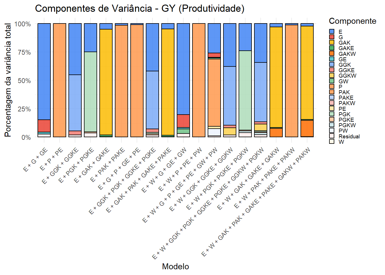

ggsave("output/variance_components/var_components_GY.tiff", p_gy, width = 12, height = 6, dpi = 300)

7.3. Gráfico para KW (Peso de Grãos)

p_kw <- variance_summary %>%
  filter(Trait == "KW") %>%
  ggplot(aes(x = Description, y = Percentage, fill = Component)) +
  geom_col(position = "fill", color = "black", alpha = 0.85, width = 0.8) +
  scale_y_continuous(labels = percent_format()) +
  scale_fill_gdocs() +
  labs(
    title = "Componentes de Variância - KW (Peso de Grãos)",
    x = "Modelo",
    y = "Porcentagem da variância total",
    fill = "Componente"
  ) +
  theme_minimal() +
  theme(
    axis.text.x = element_text(angle = 45, hjust = 1, vjust = 1, size = 8),
    legend.position = "right",
    legend.text = element_text(size = 7),
    legend.key.size = unit(0.5, "lines")
  ) +
  guides(fill = guide_legend(ncol = 1))

print(p_kw)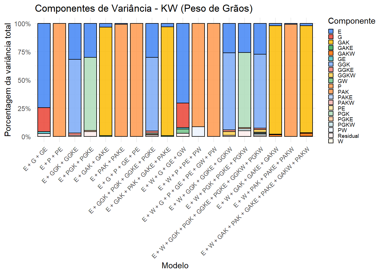

ggsave("output/variance_components/var_components_KW.tiff", p_kw, width = 12, height = 6, dpi = 300)

7.4. (Opcional) Gráfico combinado com patchwork

combined <- variance_summary %>%
  ggplot(aes(x = Description, y = Percentage, fill = Component)) +
  geom_col(position = "fill", color = "black", alpha = 0.85, width = 0.8) +
  scale_y_continuous(labels = percent_format()) +
  scale_fill_gdocs() +
  facet_wrap(~ Trait, nrow = 2) +
  labs(
    y = "Porcentagem da variância total",
    fill = "Component"
  ) +
  theme_minimal() +
  theme(
    axis.text.x = element_text(angle = 45, hjust = 1, vjust = 1, size = 8),
    legend.position = "right",
    legend.text = element_text(size = 7),
    legend.key.size = unit(0.5, "lines")
  ) +
  guides(fill = guide_legend(ncol = 1))
print(combined)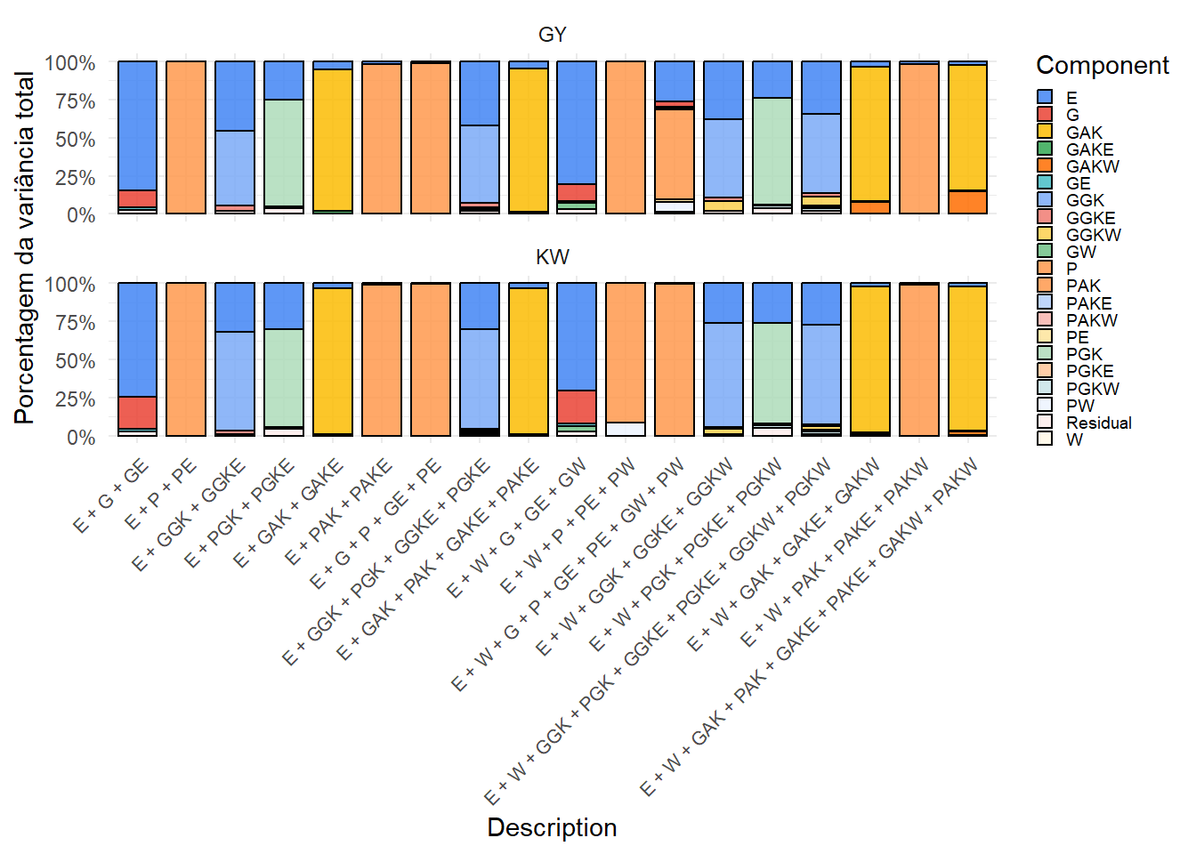

ggsave("output/variance_components/var_components_combined.tiff", combined, width = 12, height = 10, dpi = 300)

8. Considerações Finais

Os gráficos mostram a contribuição relativa de cada componente de variância nos diferentes modelos. A inclusão do kernel climático (W) e suas interações altera a partição, revelando a influência do ambiente na expressão fenotípica. Esses resultados complementam as análises de validação cruzada.

**Principais correções:**

- Adicionada verificação explícita da existência do arquivo `variance_components_raw.csv` com `stop()` caso não exista, orientando o usuário a executar a seção 6.
- Mantida a separação clara entre a etapa computacional (com `eval=FALSE`) e a etapa de visualização.
- Removidas referências a objetos não definidos (como `all_variance` no início da seção 7) – agora carregamos o arquivo.
- Ajustada a função `run_bglr_metrics` para garantir que os nomes dos componentes sejam extraídos corretamente.

Agora, ao executar o script, se o arquivo bruto não existir, ele avisará e não tentará prosseguir. Para gerar o arquivo, basta alterar o chunk `parallel-run` para `eval=TRUE` e rodar (isso pode levar horas).

<br>
<p>
<button type="button" class="btn btn-default btn-workflowr btn-workflowr-sessioninfo"
  data-toggle="collapse" data-target="#workflowr-sessioninfo"
  style = "display: block;">
  <span class="glyphicon glyphicon-wrench" aria-hidden="true"></span>
  Session information
</button>
</p>

<div id="workflowr-sessioninfo" class="collapse">

``` r
sessionInfo()

R version 4.5.1 (2025-06-13 ucrt)
Platform: x86_64-w64-mingw32/x64
Running under: Windows 11 x64 (build 26200)

Matrix products: default
  LAPACK version 3.12.1

locale:
[1] LC_COLLATE=Portuguese_Brazil.utf8  LC_CTYPE=Portuguese_Brazil.utf8   
[3] LC_MONETARY=Portuguese_Brazil.utf8 LC_NUMERIC=C                      
[5] LC_TIME=Portuguese_Brazil.utf8    

time zone: America/Sao_Paulo
tzcode source: internal

attached base packages:
[1] parallel  stats     graphics  grDevices utils     datasets  methods  
[8] base     

other attached packages:
 [1] fs_1.6.6          scales_1.4.0      ggthemes_5.2.0    doParallel_1.0.17
 [5] iterators_1.0.14  foreach_1.5.2     BGLR_1.1.4        lubridate_1.9.4  
 [9] forcats_1.0.1     stringr_1.6.0     dplyr_1.2.0       purrr_1.2.0      
[13] readr_2.1.6       tidyr_1.3.2       tibble_3.3.0      ggplot2_4.0.2    
[17] tidyverse_2.0.0  

loaded via a namespace (and not attached):
 [1] gtable_0.3.6       xfun_0.54          bslib_0.9.0        tzdb_0.5.0        
 [5] vctrs_0.7.1        tools_4.5.1        generics_0.1.4     pkgconfig_2.0.3   
 [9] RColorBrewer_1.1-3 S7_0.2.1           lifecycle_1.0.5    truncnorm_1.0-9   
[13] compiler_4.5.1     farver_2.1.2       git2r_0.36.2       textshaping_1.0.4 
[17] codetools_0.2-20   httpuv_1.6.16      htmltools_0.5.9    sass_0.4.10       
[21] yaml_2.3.12        later_1.4.4        pillar_1.11.1      crayon_1.5.3      
[25] jquerylib_0.1.4    whisker_0.4.1      MASS_7.3-65        cachem_1.1.0      
[29] tidyselect_1.2.1   digest_0.6.39      stringi_1.8.7      labeling_0.4.3    
[33] rprojroot_2.1.1    fastmap_1.2.0      grid_4.5.1         cli_3.6.5         
[37] magrittr_2.0.4     withr_3.0.2        promises_1.5.0     bit64_4.6.0-1     
[41] timechange_0.3.0   rmarkdown_2.30     bit_4.6.0          otel_0.2.0        
[45] workflowr_1.7.2    ragg_1.5.0         hms_1.1.4          evaluate_1.0.5    
[49] knitr_1.50         rlang_1.1.7        Rcpp_1.1.1         glue_1.8.0        
[53] rstudioapi_0.17.1  vroom_1.6.7        jsonlite_2.0.0     R6_2.6.1          
[57] systemfonts_1.3.1