Reproduce a paper in Rmd
Last updated: 2018-11-10
workflowr checks: (Click a bullet for more information)-
✔ R Markdown file: up-to-date
Great! Since the R Markdown file has been committed to the Git repository, you know the exact version of the code that produced these results.
-
✔ Environment: empty
Great job! The global environment was empty. Objects defined in the global environment can affect the analysis in your R Markdown file in unknown ways. For reproduciblity it’s best to always run the code in an empty environment.
-
✔ Seed:
set.seed(20181015)The command
set.seed(20181015)was run prior to running the code in the R Markdown file. Setting a seed ensures that any results that rely on randomness, e.g. subsampling or permutations, are reproducible. -
✔ Session information: recorded
Great job! Recording the operating system, R version, and package versions is critical for reproducibility.
-
Great! You are using Git for version control. Tracking code development and connecting the code version to the results is critical for reproducibility. The version displayed above was the version of the Git repository at the time these results were generated.✔ Repository version: 41b8aa2
Note that you need to be careful to ensure that all relevant files for the analysis have been committed to Git prior to generating the results (you can usewflow_publishorwflow_git_commit). workflowr only checks the R Markdown file, but you know if there are other scripts or data files that it depends on. Below is the status of the Git repository when the results were generated:
Note that any generated files, e.g. HTML, png, CSS, etc., are not included in this status report because it is ok for generated content to have uncommitted changes.Ignored files: Ignored: .DS_Store Ignored: .Rhistory Ignored: .Rproj.user/ Ignored: analysis/.DS_Store Ignored: analysis/data/ Ignored: analysis/package.Rmd Ignored: assets/ Ignored: docs/.DS_Store Untracked files: Untracked: docs/assets/Boettiger-2018-Ecology_Letters.pdf Untracked: docs/assets/Packaging-Data-Analytical Work-Reproducibly-Using-R-and-Friends.pdf Untracked: docs/css/ Untracked: libs/
Expand here to see past versions:
| File | Version | Author | Date | Message |
|---|---|---|---|---|
| html | 97818bf | annakrystalli | 2018-11-10 | Build site. |
| Rmd | 63e35ee | annakrystalli | 2018-11-10 | add link to complete compendium |
| html | 2c1e957 | annakrystalli | 2018-10-31 | Build site. |
| html | c26c936 | annakrystalli | 2018-10-31 | Build site. |
| Rmd | d3f45b6 | annakrystalli | 2018-10-31 | add intro, re-publish |
| html | 52adf4f | annakrystalli | 2018-10-30 | Build site. |
| Rmd | f7c3c51 | annakrystalli | 2018-10-30 | commit final draft |
In this section we’re going to create a literate programming document to reproduce the paper in a format suitable for journal submission or as a pre-print. We’ll do this using the course materials we downloaded.
In particular, we’re going to combine the code in analysis.R, the text in paper.txt and the references in the refs.bib file in an .Rmd document to reproduce paper.pdf.
More information on working on academic journals with Bookdown
Create journal article template using rticles
The rticles package is designed to simplify the creation of documents that conform to submission standards. A suite of custom R Markdown templates for popular journals is provided by the package.
delete paper/ subdirectory
First, let’s delete the current analysis/paper folder as we’re going to create a new paper.Rmd template.
create new paper template
This particular paper was published in Ecology Letters, an Elsevier Journal. We can create a new paper.Rmd template from the templates provided by rticles package.
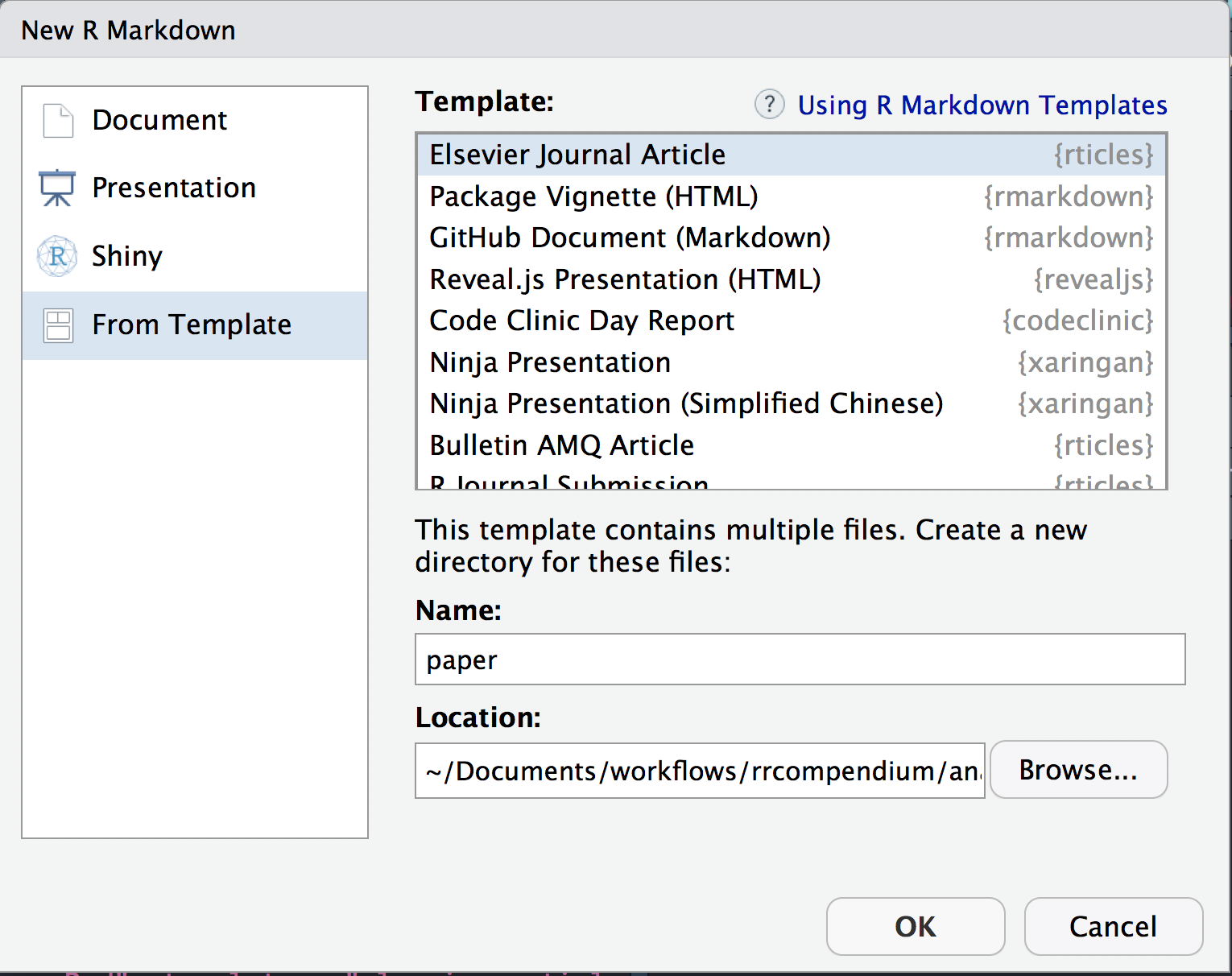
We can use the New R Markdown dialog
Select:
- Template: Elesevier Journal Article
- Name: paper
- Location:
~/Documents/workflows/rrcompendium/analysis
Or we can use rmarkdown::draft() to create articles:
Both these functions create the following files in a new directory analysis/paper.
analysis/paper
├── elsarticle.cls
├── mybibfile.bib
├── numcompress.sty
└── paper.Rmd
The
elsarticle.clscontains contains the citation language style for the references.The
mybibfile.bibcontains an example reference list.The new
paper.Rmdis the file we will be working in.
Let’s open it up and start editing it.
Update YAML
The YAML header in Paper.Rmd contains document wide metadata and is pre-populated with some fields relevant to an academic publication.
---
title: Short Paper
author:
  - name: Alice Anonymous
    email: alice@example.com
    affiliation: Some Institute of Technology
    footnote: Corresponding Author
  - name: Bob Security
    email: bob@example.com
    affiliation: Another University
address:
  - code: Some Institute of Technology
    address: Department, Street, City, State, Zip
  - code: Another University
    address: Department, Street, City, State, Zip
abstract: |
  This is the abstract.

  It consists of two paragraphs.

journal: "An awesome journal"
date: "2018-11-10"
bibliography: mybibfile.bib
output: rticles::elsevier_article
---
Here we’re going to reproduce paper.pdf as is, so we’ll actually be editing the file with details from the original publication.
First, let’s clear all text BELOW the YAML header (which is delimited by ---. DO NOT delete the YAML header).
Next, let’s open paper.txt from the course material which contains all text from the in paper.pdf. We can use it to complete some of the fields in the YAML header.
title
Add the paper title to this field
title: "From noise to knowledge: how randomness generates novel phenomena and reveals information"
address
Here we specify the addresses associated with the affiliations specified in authors
address:
  - code: a
    address: "Dept of Environmental Science, Policy, and Management, University of California Berkeley, Berkeley CA 94720-3114, USA"
Note that the field code in address cross-references with the affiliations specified in author.
bibliography
Before specifying the bibliography, we need to copy the refs.bib file associated with paper.pdf from the course materials and save it in our analysis/paper subdirectory.
Next we can set the refs.bib as the source for our paper’s bibliograpraphy:
bibliography: refs.biblayout
We can add an additional field called layout which specifies the layout of the output and takes the following values.
- review: doublespace margins
- 3p: singlespace margins
- 5p: two-column
Let’s use singlespace margins
layout: 3ppreamble
We can add also an additional field called preamble. This allows us to include LaTeX packages and functions. We’ll use the following to add linenumbers and doublespacing.
preamble: |
  \usepackage[nomarkers]{endfloat}
  \linenumbers
  \usepackage{setspace}
  \doublespacing
abstract
This field should contain the abstract
abstract: |

  # Abstract

  Noise, as the term itself suggests, is most often seen a nuisance to ecological insight, a inconvenient reality that must be acknowledged, a haystack that must be stripped away to reveal the processes of interest underneath. Yet despite this well-earned reputation, noise is often interesting in its own right: noise can induce novel phenomena that could not be understood from some underlying determinstic model alone.  Nor is all noise the same, and close examination of differences in frequency, color or magnitude can reveal insights that would otherwise be inaccessible.  Yet with each aspect of stochasticity leading to some new or unexpected behavior, the time is right to move beyond the familiar refrain of "everything is important" (Bjørnstad & Grenfell 2001).  Stochastic phenomena can suggest new ways of inferring process from pattern, and thus spark more dialog between theory and empirical perspectives that best advances the field as a whole. I highlight a few compelling examples, while observing that the study of stochastic phenomena are only beginning to make this translation into empirical inference.  There are rich opportunities at this interface in the years ahead.
output
The output format. In this case, the template is correctly pre-populated with rticles::elsevier_article so no need to edit.
output: rticles::elsevier_articleAdd text
Now let’s add the main body of the paper from paper.txt.
add new page after abstract
First, let’s a add a new page after the abstract using:
\newpage
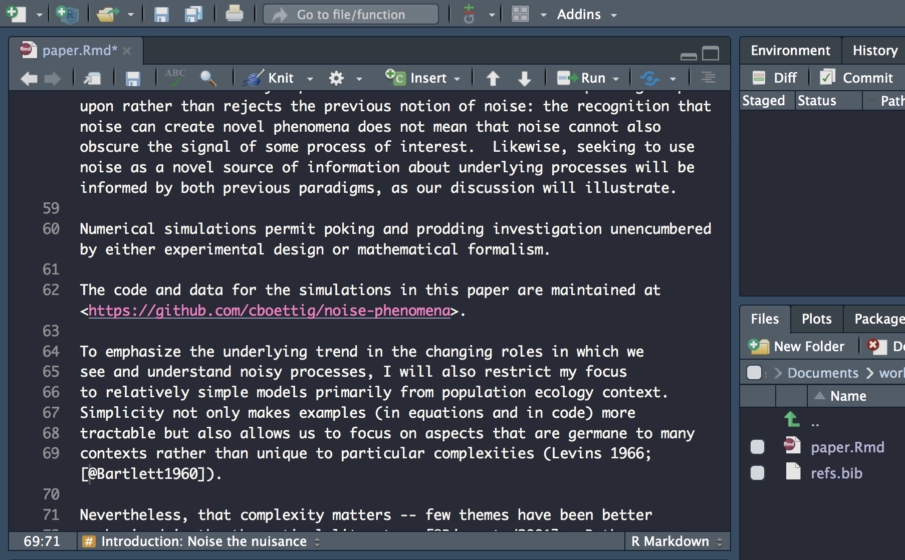
copy and paste text from paper.txt
We do not need the details we’ve just completed the YAML with, so ignore the title, abstract etc and just copy everything in paper.txt from the Introduction header down to and including the reference section header.
# Introduction: Noise the nuisance

To many, stochasticity, or more simply, noise,
is just that -- something which obscures patterns we are

...
...
...
...
...

# Acknowledgements

The author acknowledges feedback and advice from the editor,
Tim Coulson and two anonymous reviewers. This work was supported in
part by  USDA National Institute of Food and Agriculture, Hatch
project CA-B-INS-0162-H.

# References
Check pdf output
Let’s knit our document and have our first look at the resulting pdf by clicking on the Knit tab.
Update references
Next we’ll replace the flat citations in the text with real linked citation which can be used to auto-generate formatted inline citations and the references section.
Insert formatted citations
We’ll use the citr package, which provides functions and an RStudio addin to search a BibTeX-file to create and insert formatted Markdown citations into the current document.
Once citr is installed and you have restarted your R session, the addin appears in the addin menu. The addin will automatically look up the Bib(La)TeX-file(s) specified in the YAML front matter.
To insert a citation
Select text to replace with a citation
Launch
citraddin: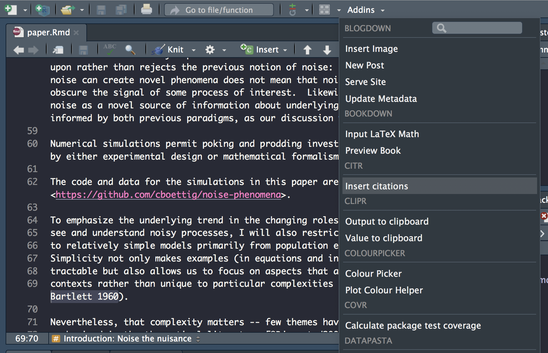
Search for citation to insert
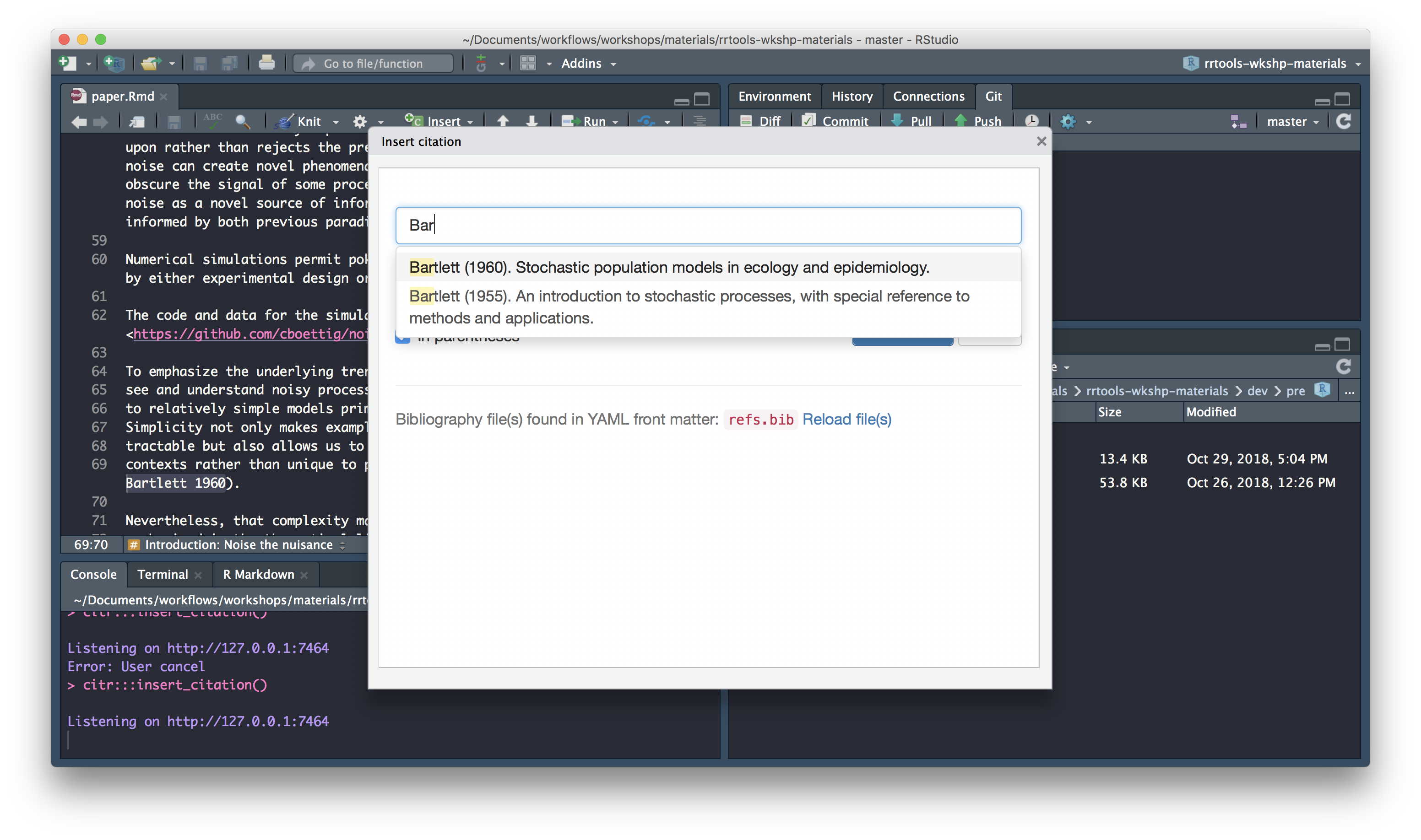
Select citation to insert
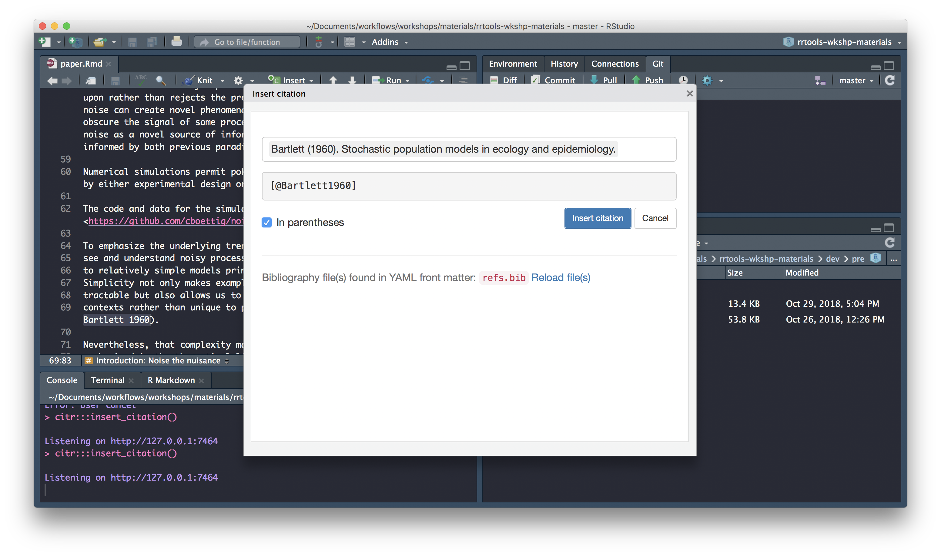
Insert citation
Carry on updating the rest of the citations. Don’t forget to check the abstract for citations!
Update math
For the sake of time today, and not to open this topic too deeply here, I’ve included the following LaTex equation syntax in the text:
\begin{align}
\frac{\mathrm{d} n}{\mathrm{d} t} = \underbrace{c n \left(1 - \frac{n}{N}\right)}_{\textrm{birth}} - \underbrace{e n}_{\textrm{death}}, \label{levins}
\end{align}
that generates equation 1 in the paper.pdf.
\[\begin{align} \frac{\mathrm{d} n}{\mathrm{d} t} = \underbrace{c n \left(1 - \frac{n}{N}\right)}_{\textrm{birth}} - \underbrace{e n}_{\textrm{death}}, \label{levins} \end{align}\]
So you don’t need to edit anything here.
Check Math expressions and Markdown extensions by bookdown for more information.
update inline math
Inline LaTeX equations and parameters can be written between a pair of dollar signs using the LaTeX syntax, e.g., $f(x) = 1/x$ generates \(f(x) = 1/x\).
Using paper.pdf to identify mathematical expressions in the text (generally they appear in italic), edit your paper.Rmd, enclosing them between dollar signs.
Check pdf output
Let’s knit our document to check our references and maths annotations have been updated correctly by clicking on the Knit tab.
Add code
Now that we’ve set up the text for our paper, let’s insert the code to generate figure 1.
Add libraries chunk
First let’s insert a libraries code chunk right at the top of the document to set up our analysis. Because it’s a setup chunk we set include = F which suppresses all output resulting from chunk evaluation.
  ```{r libraries, include=FALSE}

 ```
set document chunk options
Now, let’s set some knitr options for the whole document by adding the following code to our libraries chunk:
knitr::opts_chunk$set(echo = FALSE, message=FALSE, warning=FALSE,
                      dev="cairo_pdf", fig.width=7, fig.height=3.5)
We’re setting default chunk options to:
echo = FALSEmessage = FALSEwarning = FALSE
to suppress code, warnings and messages in the output, and
dev="cairo_pdf"fig.width=7fig.height=3.5
to specify how figures will appear.
add libraries
Copy and paste the code for loading all the libraries from analysis.R. Add library rrcompendium so we can access function recode_system_size. The libraries chunk should now look like so:
knitr::opts_chunk$set(echo = FALSE, message=FALSE, warning=FALSE,
                      dev="cairo_pdf", fig.width=7, fig.height=3.5)

library(dplyr)
library(readr)
library(ggplot2)
library(ggthemes)
library(rrcompendium)
Add set-theme chunk
Right below the libraries chunk, insert a new chunk and call it set-theme
Copy the code to set the plot theme and pasted into the set-theme code:
Add figure1 chunk
Now scroll down towards the bottom of the document and create a new chunk just above the Conclusions section. Call it figure1
Add code
Copy and paste the remaining code into a new chunk which will create figure 1.
# create colour palette
colours <- ptol_pal()(2)

# load-data
data <- read_csv(here::here("gillespie.csv"), col_types = "cdiddd")

# recode-data
data <- data %>%
  mutate(system_size = recode(system_size, large = "A. 1000 total sites", small= "B. 100 total sites"))

# plot-gillespie
data %>%
  ggplot(aes(x = time)) +
  geom_hline(aes(yintercept = mean), lty=2, col=colours[2]) +
  geom_hline(aes(yintercept = minus_sd), lty=2, col=colours[2]) +
  geom_hline(aes(yintercept = plus_sd), lty=2, col=colours[2]) +
  geom_line(aes(y = n), col=colours[1]) +
  facet_wrap(~system_size, scales = "free_y")
edit code
Edit the code to
update the path to
gillespie.csvstreamline the code to a single pipe to include
recode_system_size
read_csv(here::here("analysis", "data","raw_data", "gillespie.csv"),
         col_types = "cdiddd")  %>%
    # recode-data
    recode_system_size() %>%
    # plot-gillespie
    ggplot(aes(x = time)) +
    geom_hline(aes(yintercept = mean), lty=2, col=colours[2]) +
    geom_hline(aes(yintercept = minus_sd), lty=2, col=colours[2]) +
    geom_hline(aes(yintercept = plus_sd), lty=2, col=colours[2]) +
    geom_line(aes(y = n), col=colours[1]) +
    facet_wrap(~system_size, scales = "free_y")
Add caption
Finally, let’s update chunk figure1 to include a figure caption. The text for the caption is at the bottom of paper.txt. We can include it in the chunk header through chunk option fig.cap like so:
```{r figure1, figure1, fig.cap="Population dynamics from a Gillespie simulation of the Levins model with large (N=1000, panel A) and small (N=100, panel B) number of sites (blue) show relatively weaker effects of demographic noise in the bigger system. Models are otherwise identical, with e = 0.2 and c = 1 (code in appendix A). Theoretical predictions for mean and plus/minus one standard deviation shown in horizontal re dashed lines."} ```Render final document to pdf
Let’s check our final work by re-knitting to pdf. You should be looking at something that looks a lot like paper.pdf
Add paper dependencies
Finally, before we’re finished, let’s ensure the additional dependencies introduced in the paper are included. We can use rrtools::add_dependencies_to_description()
This function scans script files (.R, .Rmd, .Rnw, .Rpres, etc.) for external package dependencies indicated by library(), require() or :: and adds those packages to the Imports field in the package DESCRIPTION:
Imports:
    bookdown,
    dplyr,
    ggplot2 (>= 3.0.0),
    ggthemes (>= 3.5.0),
    here (>= 0.1),
    knitr (>= 1.20),
    rticles (>= 0.6)
🔨 Install and Restart
Commit and push to GitHub!
Final compendium
You can see the resulting rrcompendium here
The complete compendium should contain the following files:
.
├── CONDUCT.md
├── CONTRIBUTING.md
├── DESCRIPTION
├── LICENSE
├── LICENSE.md
├── NAMESPACE
├── R
│   └── process-data.R
├── README.Rmd
├── README.md
├── analysis
│   ├── data
│   │   ├── DO-NOT-EDIT-ANY-FILES-IN-HERE-BY-HAND
│   │   ├── derived_data
│   │   └── raw_data
│   │       └── gillespie.csv
│   ├── figures
│   ├── paper
│   │   ├── elsarticle.cls
│   │   ├── mybibfile.bib
│   │   ├── numcompress.sty
│   │   ├── paper.Rmd
│   │   ├── paper.fff
│   │   ├── paper.pdf
│   │   ├── paper.spl
│   │   ├── paper.tex
│   │   ├── paper_files
│   │   │   └── figure-latex
│   │   │       └── figure1-1.pdf
│   │   └── refs.bib
│   └── templates
│       ├── journal-of-archaeological-science.csl
│       ├── template.Rmd
│       └── template.docx
├── inst
│   └── testdata
│       └── gillespie.csv
├── man
│   └── recode_system_size.Rd
├── rrcompendium.Rproj
└── tests
    ├── testthat
    │   └── test-process-data.R
    └── testthat.R
Session information
This reproducible R Markdown analysis was created with workflowr 1.1.1