Introduction to R
Anthony Hung
2019-04-25
Last updated: 2019-05-27
Checks: 6 0
Knit directory: MSTPsummerstatistics/
This reproducible R Markdown analysis was created with workflowr (version 1.3.0). The Checks tab describes the reproducibility checks that were applied when the results were created. The Past versions tab lists the development history.
Great! Since the R Markdown file has been committed to the Git repository, you know the exact version of the code that produced these results.
Great job! The global environment was empty. Objects defined in the global environment can affect the analysis in your R Markdown file in unknown ways. For reproduciblity it’s best to always run the code in an empty environment.
The command set.seed(20180927) was run prior to running the code in the R Markdown file. Setting a seed ensures that any results that rely on randomness, e.g. subsampling or permutations, are reproducible.
Great job! Recording the operating system, R version, and package versions is critical for reproducibility.
Nice! There were no cached chunks for this analysis, so you can be confident that you successfully produced the results during this run.
Great! You are using Git for version control. Tracking code development and connecting the code version to the results is critical for reproducibility. The version displayed above was the version of the Git repository at the time these results were generated.
Note that you need to be careful to ensure that all relevant files for the analysis have been committed to Git prior to generating the results (you can use wflow_publish or wflow_git_commit). workflowr only checks the R Markdown file, but you know if there are other scripts or data files that it depends on. Below is the status of the Git repository when the results were generated:
Ignored files:
    Ignored:    .DS_Store
    Ignored:    .Rhistory
    Ignored:    .Rproj.user/
    Ignored:    analysis/.RData
    Ignored:    analysis/.Rhistory
Note that any generated files, e.g. HTML, png, CSS, etc., are not included in this status report because it is ok for generated content to have uncommitted changes.
These are the previous versions of the R Markdown and HTML files. If you’ve configured a remote Git repository (see ?wflow_git_remote), click on the hyperlinks in the table below to view them.
| File | Version | Author | Date | Message |
|---|---|---|---|---|
| html | b291d24 | Anthony Hung | 2019-05-24 | Build site. |
| html | 4e210d6 | Anthony Hung | 2019-05-24 | Build site. |
| html | c4bdfdc | Anthony Hung | 2019-05-22 | Build site. |
| Rmd | dd1e411 | Anthony Hung | 2019-05-22 | before republishing syllabus |
| html | dd1e411 | Anthony Hung | 2019-05-22 | before republishing syllabus |
| Rmd | 4ce8e85 | Anthony Hung | 2019-05-21 | bandersnatch add |
| html | 4ce8e85 | Anthony Hung | 2019-05-21 | bandersnatch add |
| html | 096760a | Anthony Hung | 2019-05-18 | Build site. |
| html | da98ae8 | Anthony Hung | 2019-05-17 | Build site. |
| html | bb90220 | Anthony Hung | 2019-05-17 | commit before publishing |
| Rmd | 239723e | Anthony Hung | 2019-05-08 | Update learning objectives |
| html | 239723e | Anthony Hung | 2019-05-08 | Update learning objectives |
| html | 2ec7944 | Anthony Hung | 2019-05-06 | Build site. |
| html | 536085f | Anthony Hung | 2019-05-06 | Build site. |
| html | ee75486 | Anthony Hung | 2019-05-04 | Build site. |
| html | 5ea5f30 | Anthony Hung | 2019-04-29 | Build site. |
| html | e0e8156 | Anthony Hung | 2019-04-29 | Build site. |
| html | e746cf5 | Anthony Hung | 2019-04-28 | Build site. |
| Rmd | 133df4a | Anthony Hung | 2019-04-28 | introR |
| html | 133df4a | Anthony Hung | 2019-04-28 | introR |
| html | 22b3720 | Anthony Hung | 2019-04-26 | Build site. |
| html | ddb3114 | Anthony Hung | 2019-04-26 | Build site. |
| html | 413d065 | Anthony Hung | 2019-04-26 | Build site. |
| html | 6b98d6c | Anthony Hung | 2019-04-26 | Build site. |
| Rmd | 9f13e70 | Anthony Hung | 2019-04-25 | finish CLT |
| html | 9f13e70 | Anthony Hung | 2019-04-25 | finish CLT |
Introduction
Here, we introduce R, a statistical programming language. Doing statistics within a programming language brings many advantages, including allowing one to organize all analyses into program files that can be rerun to replicate analyses. In addition to using R, we will be using RStudio, an integrated development environment (IDE), which assists us in working with R and outputs of our code as we develop it. Our objective today is to get everyone up to speed with working knowledge of R and programming to be able to do exercises as a part of the rest of the course.
Both R and RStudio are freely available online.
Downloading/Installing R and RStudio
Download the appropriate “base” version of R for your operating system from CRAN: https://cran.r-project.org/
Install the software with default settings.
Download the appropriate RStudio version for your operating system: https://www.rstudio.com/products/rstudio/download/#download
R Basics
Follow along in your R console with the code in each of the code chunks as we explore the different aspects of R! Clicking on the github logo on the top right corner of the webpage will take you to the repository for this website, where you can download the R markdown file for this page to load into RStudio to follow along.
Mathematical operations in R
Many familiar operators work in R, allowing you to work with numbers like you would in a calculator. Operators such as inequalities also work, returning “TRUE” if the proposed logical expression is true and “FALSE” otherwise.
2+4 #addition[1] 62-4 #subtraction[1] -22*4 #multiplication[1] 82/4 #division[1] 0.52^4 #exponentiation[1] 16log(2) #the default log base is the natural log[1] 0.69314722 < 4[1] TRUE2 > 4[1] FALSE2 >= 4 #greater than or equal to [1] FALSE2 == 2 #is equal to (notice that there are two equal signs, as a single equal sign denotes assignment)[1] TRUE2 != 4 #is not equal to [1] TRUE2 != 4 | 2 + 2 == 4 #OR[1] TRUE2 != 4 & 2 + 2 == 4 #AND[1] TRUE"Red" == "Red"[1] TRUEObjects
In addition to being able to work with actual numbers, R works in objects, which can represent anything from numbers to strings to vectors to matrices. Everything in R is an object. The best practice for assigning variable names to objects is the “<-” operator. After objects are created, they are stored in in the “Environment” tab in your RStudio console and can be called upon to perform different operations.
R has many data structures, including:
- atomic vector
- list
- matrix
- data frame
- factors
R has 6 atomic vector types, or classes. Atomic means that a vector only contains elements of one class (i.e. the elements inside the vector do not come from mutliple classes).
- character
- numeric (real or decimal)
- integer
- logical (TRUE or FALSE)
- complex (containing i)
a <- 2
b <- 3
a + b
[1] 5class(a) #the "class" function tells you what class of object a is[1] "numeric"d <- c(1,2,3,4,5) #the "c" function concatenates the arguments contained within it into a vector
d[1] 1 2 3 4 5d <- c(d, 1) #The "c" function also allows you to append items to an existing vector
d[1] 1 2 3 4 5 1class(d)[1] "numeric"d[3] #brackets allow you index vectors or matrices. Here, we call the third value from our d vector.[1] 3#Matrices are just like vectors, but with two dimensions
my_matrix <- matrix(seq(1:9), ncol = 3)
my_matrix [,1] [,2] [,3]
[1,] 1 4 7
[2,] 2 5 8
[3,] 3 6 9#vectors and matrices can only contain objects of one class. If you include objects of multiple types into the same vector, R will perform coersion to force all the objects contained in the vector into a shared class
x <- c(1.7, "a")
x[1] "1.7" "a" class("a")[1] "character"class(1.7)[1] "numeric"class(x)[1] "character"y <- c(TRUE, 2)
y[1] 1 2z <- c("a", TRUE)
z[1] "a" "TRUE"#If you would like to store objects of multiple classes into one object, a list can accomodate such a task.
x_y_z_list <- list(x,y,z)
x_y_z_list[[1]]
[1] "1.7" "a"
[[2]]
[1] 1 2
[[3]]
[1] "a" "TRUE"#to index an element in a list, use double brackets [[]]. You can further index elements within an element of a list.
x_y_z_list[[1]][1] "1.7" "a" x_y_z_list[[1]][2][1] "a"#elements in a list can be assigned names
x_y_z_list <- list(a=x, b=y, c=z)
x_y_z_list$a
[1] "1.7" "a"
$b
[1] 1 2
$c
[1] "a" "TRUE"#Dataframes are a very commonly used type of object in R. You can think of a dataframe as a rectangular combination of lists.
#The below code stores the stated values in a dataframe which contains employee ids, names, salaries, and start dates for 5 employees
emp.data <- data.frame(
emp_id = c (1:5),
emp_name = c("Rick","Dan","Michelle","Ryan","Gary"),
salary = c(623.3,515.2,611.0,729.0,843.25),
start_date = as.Date(c("2012-01-01", "2013-09-23", "2014-11-15", "2014-05-11",
"2015-03-27")),
stringsAsFactors = FALSE
)
emp.data emp_id emp_name salary start_date
1 1 Rick 623.30 2012-01-01
2 2 Dan 515.20 2013-09-23
3 3 Michelle 611.00 2014-11-15
4 4 Ryan 729.00 2014-05-11
5 5 Gary 843.25 2015-03-27emp.data$emp_id #the $ operator calls on a certain column of a dataframe[1] 1 2 3 4 5class(emp.data$emp_id) #As noted earlier, a dataframe can be thought of as a rectangular list, combining different data classes together, each in a different column.[1] "integer"class(emp.data$salary)[1] "numeric"emp.data$emp_name[emp.data$salary > 620] #You can combine logical operators, brackets, and the $ sign to subset your dataframe in any way you choose! Here, we print out all the employee names for employees who have a salary greater than 620.[1] "Rick" "Ryan" "Gary"ls() #ls lists all the variable names that have been assigned to objects in your workspace[1] "a" "b" "d" "emp.data" "my_matrix"
[6] "x" "x_y_z_list" "y" "z" Using Packages in R
In addition to the basic functions provided in R, oftentimes we will be working with packages that contain functions written by other people to perform common tasks or specific analyses. Packages can also contain datasets. We can load these packages into our R environment after installing them in R.
usePackage <- function(p)
{
  if (!is.element(p, installed.packages()[,1]))
    install.packages(p, dep = TRUE)
  require(p, character.only = TRUE)
}

usePackage("gapminder")#This code installs the gapminder packages, which contains vital statistics data from multiple countries. install.packages() is the function that will install a package for you if you know it's name.
Loading required package: gapminderlibrary("gapminder") #After installing the package, we need to tell R to load it into our current environment with this function.
head(gapminder) #The package gapminder contains a dataset called gapminder. We can use the "head" function to print out the first 6 rows of this dataset.# A tibble: 6 x 6
country continent year lifeExp pop gdpPercap
<fct> <fct> <int> <dbl> <int> <dbl>
1 Afghanistan Asia 1952 28.8 8425333 779.
2 Afghanistan Asia 1957 30.3 9240934 821.
3 Afghanistan Asia 1962 32.0 10267083 853.
4 Afghanistan Asia 1967 34.0 11537966 836.
5 Afghanistan Asia 1972 36.1 13079460 740.
6 Afghanistan Asia 1977 38.4 14880372 786.?gapminder #the ? operator lauches a help page to describe a particular function, including the arguments it takes. Whenever using a new function, it is good practice to first explore it through ?.Loops
Oftentimes, we may want to perform the same operation or function many many times. Rather than having to explicitly write out each individual operation, we can make use of loops. For example, let’s say that we want to raise the number 2 to the power of each integer from 0 to 20. We could either write out 2^0, 2^1, 2^2 …, or make use of a for loop to condense our code while getting the same result.
2^0[1] 12^1[1] 22^2[1] 42^3[1] 8# ...
#This is a for loop. in the parentheses after the for function, we specify over what range of values we want to loop over, and assign a dummy variable name to take on each of those values in sequence. Within the curly braces, we state what operation we want to perform over all the values taken on by the dummy variable.
for(i in 0:20){
print(2^i)
}[1] 1
[1] 2
[1] 4
[1] 8
[1] 16
[1] 32
[1] 64
[1] 128
[1] 256
[1] 512
[1] 1024
[1] 2048
[1] 4096
[1] 8192
[1] 16384
[1] 32768
[1] 65536
[1] 131072
[1] 262144
[1] 524288
[1] 1048576User-defined Functions (UDF)
Another way to avoid writing out or copy-pasting the same exact thing over and over again when working with data is to write a function to contain a certain combination of operations you find yourself running mutliple times. For example, you may find yourself needing to calculate the Hardy-Weinberg Equillibrium genotype frequencies of a population given the allele frequencies. We can wrap up all the code that you would need to calculate this in a function that we can call upon again and again.
calc_HWE_geno <- function(p = 0.5){
  q <- 1-p

  pp <- p^2
  pq <- 2*p*q
  qq <- q^2

  return(c(pp, pq, qq))
}

calc_HWE_geno(p = 0.1)
[1] 0.01 0.18 0.81#note that in our UDF we assigned a default value to p (p = 0.5). This means that if we do not specify a value for our argument of p, it will default to using that value.
calc_HWE_geno()[1] 0.25 0.50 0.25Plots
In addition to mathematical operations, R can help with data visualization. Base R has a few useful plotting functions, but popular packages such as ggplot2 give more customization and control to the user.
hist(gapminder$lifeExp)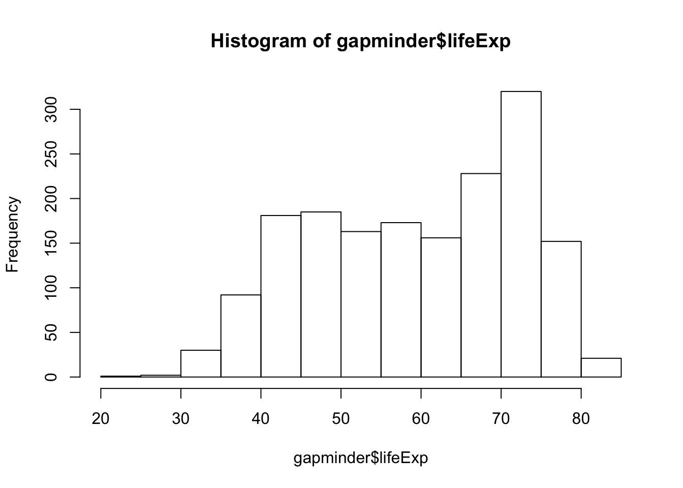
| Version | Author | Date |
|---|---|---|
| 133df4a | Anthony Hung | 2019-04-28 |
boxplot(lifeExp ~ continent, data = gapminder) #box plot for the life expectancies of all years per continent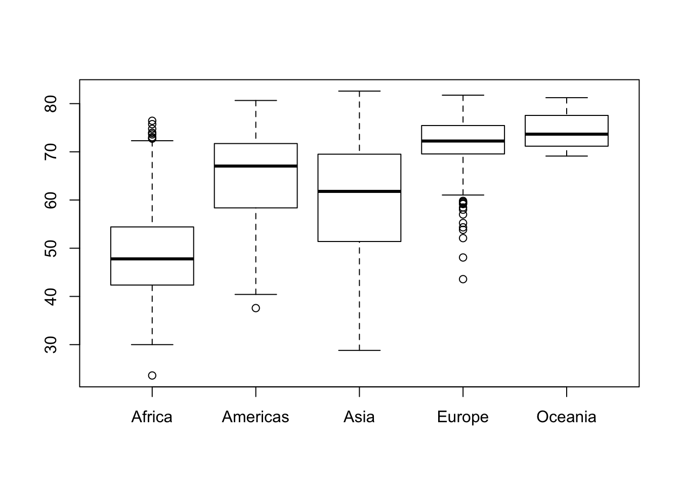
| Version | Author | Date |
|---|---|---|
| 133df4a | Anthony Hung | 2019-04-28 |
Setting a random seed
R has many functions that use a random number generator to generate an output. For example, the r____ functions (e.g. rbinom, runif) pull numbers from a probability distribution of your choice. In order to create reproducible analyses, it is often advantageous to be able to reliably obtain the same “random” number after running the same function over again. In order to do so, we can set a seed for the random number generator.
runif(1,0,1) #runif pulls a number from the uniform distribution with a set of given parameters[1] 0.1944457runif(1,0,1) #we can see that running runif twice gives you differnt results[1] 0.205278set.seed(1234) #setting a seed allows us to obtain reproducible results from functions that use the random number generator
runif(1,0,1)[1] 0.1137034set.seed(1234)
runif(1,0,1)[1] 0.1137034Reading and writing data in R
Finally, let us address probably one of the most important points when working with statistics in science: how to get the data you have collected into your R environment. For this part of the lesson, we will be working with the bandersnatch.csv file (created by Katie Long) located here: https://raw.githubusercontent.com/anthonyhung/MSTPsummerstatistics/master/data/bandersnatch.csv. If you would like to have your own copy of this dataset, you can open up a terminal window and run the commands.
cd ~/Desktop
mkdir data
cd data
wget https://raw.githubusercontent.com/anthonyhung/MSTPsummerstatistics/master/data/bandersnatch.csv
mkdir: data: File exists
--2019-05-27 21:07:24-- https://raw.githubusercontent.com/anthonyhung/MSTPsummerstatistics/master/data/bandersnatch.csv
Resolving raw.githubusercontent.com... 151.101.184.133
Connecting to raw.githubusercontent.com|151.101.184.133|:443... connected.
HTTP request sent, awaiting response... 200 OK
Length: 13511471 (13M) [text/plain]
Saving to: ‘bandersnatch.csv.7’
0K .......... .......... .......... .......... .......... 0% 1.67M 8s
50K .......... .......... .......... .......... .......... 0% 4.39M 5s
100K .......... .......... .......... .......... .......... 1% 7.71M 4s
150K .......... .......... .......... .......... .......... 1% 4.19M 4s
200K .......... .......... .......... .......... .......... 1% 3.60M 4s
250K .......... .......... .......... .......... .......... 2% 3.81M 4s
300K .......... .......... .......... .......... .......... 2% 3.46M 4s
350K .......... .......... .......... .......... .......... 3% 2.89M 4s
400K .......... .......... .......... .......... .......... 3% 3.65M 4s
450K .......... .......... .......... .......... .......... 3% 3.45M 4s
500K .......... .......... .......... .......... .......... 4% 4.07M 4s
550K .......... .......... .......... .......... .......... 4% 3.30M 4s
600K .......... .......... .......... .......... .......... 4% 4.09M 4s
650K .......... .......... .......... .......... .......... 5% 3.48M 4s
700K .......... .......... .......... .......... .......... 5% 3.76M 3s
750K .......... .......... .......... .......... .......... 6% 2.70M 4s
800K .......... .......... .......... .......... .......... 6% 3.36M 4s
850K .......... .......... .......... .......... .......... 6% 4.17M 3s
900K .......... .......... .......... .......... .......... 7% 3.34M 3s
950K .......... .......... .......... .......... .......... 7% 4.02M 3s
1000K .......... .......... .......... .......... .......... 7% 3.61M 3s
1050K .......... .......... .......... .......... .......... 8% 3.71M 3s
1100K .......... .......... .......... .......... .......... 8% 3.54M 3s
1150K .......... .......... .......... .......... .......... 9% 2.68M 3s
1200K .......... .......... .......... .......... .......... 9% 3.58M 3s
1250K .......... .......... .......... .......... .......... 9% 3.61M 3s
1300K .......... .......... .......... .......... .......... 10% 3.54M 3s
1350K .......... .......... .......... .......... .......... 10% 3.79M 3s
1400K .......... .......... .......... .......... .......... 10% 3.83M 3s
1450K .......... .......... .......... .......... .......... 11% 3.50M 3s
1500K .......... .......... .......... .......... .......... 11% 3.79M 3s
1550K .......... .......... .......... .......... .......... 12% 2.81M 3s
1600K .......... .......... .......... .......... .......... 12% 3.32M 3s
1650K .......... .......... .......... .......... .......... 12% 3.89M 3s
1700K .......... .......... .......... .......... .......... 13% 3.56M 3s
1750K .......... .......... .......... .......... .......... 13% 3.60M 3s
1800K .......... .......... .......... .......... .......... 14% 3.76M 3s
1850K .......... .......... .......... .......... .......... 14% 3.40M 3s
1900K .......... .......... .......... .......... .......... 14% 2.69M 3s
1950K .......... .......... .......... .......... .......... 15% 3.90M 3s
2000K .......... .......... .......... .......... .......... 15% 3.44M 3s
2050K .......... .......... .......... .......... .......... 15% 3.63M 3s
2100K .......... .......... .......... .......... .......... 16% 3.80M 3s
2150K .......... .......... .......... .......... .......... 16% 3.86M 3s
2200K .......... .......... .......... .......... .......... 17% 2.60M 3s
2250K .......... .......... .......... .......... .......... 17% 6.23M 3s
2300K .......... .......... .......... .......... .......... 17% 2.71M 3s
2350K .......... .......... .......... .......... .......... 18% 3.49M 3s
2400K .......... .......... .......... .......... .......... 18% 3.83M 3s
2450K .......... .......... .......... .......... .......... 18% 3.35M 3s
2500K .......... .......... .......... .......... .......... 19% 3.87M 3s
2550K .......... .......... .......... .......... .......... 19% 3.73M 3s
2600K .......... .......... .......... .......... .......... 20% 3.30M 3s
2650K .......... .......... .......... .......... .......... 20% 3.69M 3s
2700K .......... .......... .......... .......... .......... 20% 2.79M 3s
2750K .......... .......... .......... .......... .......... 21% 3.69M 3s
2800K .......... .......... .......... .......... .......... 21% 3.79M 3s
2850K .......... .......... .......... .......... .......... 21% 3.79M 3s
2900K .......... .......... .......... .......... .......... 22% 3.41M 3s
2950K .......... .......... .......... .......... .......... 22% 3.69M 3s
3000K .......... .......... .......... .......... .......... 23% 3.34M 3s
3050K .......... .......... .......... .......... .......... 23% 3.61M 3s
3100K .......... .......... .......... .......... .......... 23% 2.55M 3s
3150K .......... .......... .......... .......... .......... 24% 3.50M 3s
3200K .......... .......... .......... .......... .......... 24% 3.67M 3s
3250K .......... .......... .......... .......... .......... 25% 3.69M 3s
3300K .......... .......... .......... .......... .......... 25% 3.48M 3s
3350K .......... .......... .......... .......... .......... 25% 3.47M 3s
3400K .......... .......... .......... .......... .......... 26% 3.66M 3s
3450K .......... .......... .......... .......... .......... 26% 3.93M 3s
3500K .......... .......... .......... .......... .......... 26% 2.68M 3s
3550K .......... .......... .......... .......... .......... 27% 3.91M 3s
3600K .......... .......... .......... .......... .......... 27% 3.65M 3s
3650K .......... .......... .......... .......... .......... 28% 3.11M 3s
3700K .......... .......... .......... .......... .......... 28% 3.84M 3s
3750K .......... .......... .......... .......... .......... 28% 3.22M 3s
3800K .......... .......... .......... .......... .......... 29% 3.46M 3s
3850K .......... .......... .......... .......... .......... 29% 3.76M 3s
3900K .......... .......... .......... .......... .......... 29% 2.72M 3s
3950K .......... .......... .......... .......... .......... 30% 3.25M 3s
4000K .......... .......... .......... .......... .......... 30% 4.12M 3s
4050K .......... .......... .......... .......... .......... 31% 3.71M 3s
4100K .......... .......... .......... .......... .......... 31% 3.18M 3s
4150K .......... .......... .......... .......... .......... 31% 3.83M 3s
4200K .......... .......... .......... .......... .......... 32% 3.66M 3s
4250K .......... .......... .......... .......... .......... 32% 3.11M 3s
4300K .......... .......... .......... .......... .......... 32% 3.00M 2s
4350K .......... .......... .......... .......... .......... 33% 3.43M 2s
4400K .......... .......... .......... .......... .......... 33% 3.25M 2s
4450K .......... .......... .......... .......... .......... 34% 3.36M 2s
4500K .......... .......... .......... .......... .......... 34% 3.99M 2s
4550K .......... .......... .......... .......... .......... 34% 3.27M 2s
4600K .......... .......... .......... .......... .......... 35% 3.86M 2s
4650K .......... .......... .......... .......... .......... 35% 3.57M 2s
4700K .......... .......... .......... .......... .......... 35% 2.66M 2s
4750K .......... .......... .......... .......... .......... 36% 3.70M 2s
4800K .......... .......... .......... .......... .......... 36% 3.61M 2s
4850K .......... .......... .......... .......... .......... 37% 3.71M 2s
4900K .......... .......... .......... .......... .......... 37% 3.61M 2s
4950K .......... .......... .......... .......... .......... 37% 3.53M 2s
5000K .......... .......... .......... .......... .......... 38% 3.48M 2s
5050K .......... .......... .......... .......... .......... 38% 3.25M 2s
5100K .......... .......... .......... .......... .......... 39% 2.44M 2s
5150K .......... .......... .......... .......... .......... 39% 3.64M 2s
5200K .......... .......... .......... .......... .......... 39% 3.92M 2s
5250K .......... .......... .......... .......... .......... 40% 3.52M 2s
5300K .......... .......... .......... .......... .......... 40% 3.37M 2s
5350K .......... .......... .......... .......... .......... 40% 3.57M 2s
5400K .......... .......... .......... .......... .......... 41% 3.63M 2s
5450K .......... .......... .......... .......... .......... 41% 3.69M 2s
5500K .......... .......... .......... .......... .......... 42% 2.73M 2s
5550K .......... .......... .......... .......... .......... 42% 3.59M 2s
5600K .......... .......... .......... .......... .......... 42% 3.99M 2s
5650K .......... .......... .......... .......... .......... 43% 3.42M 2s
5700K .......... .......... .......... .......... .......... 43% 3.62M 2s
5750K .......... .......... .......... .......... .......... 43% 3.59M 2s
5800K .......... .......... .......... .......... .......... 44% 3.14M 2s
5850K .......... .......... .......... .......... .......... 44% 3.21M 2s
5900K .......... .......... .......... .......... .......... 45% 2.88M 2s
5950K .......... .......... .......... .......... .......... 45% 3.57M 2s
6000K .......... .......... .......... .......... .......... 45% 3.29M 2s
6050K .......... .......... .......... .......... .......... 46% 3.87M 2s
6100K .......... .......... .......... .......... .......... 46% 3.39M 2s
6150K .......... .......... .......... .......... .......... 46% 3.50M 2s
6200K .......... .......... .......... .......... .......... 47% 3.92M 2s
6250K .......... .......... .......... .......... .......... 47% 3.74M 2s
6300K .......... .......... .......... .......... .......... 48% 2.58M 2s
6350K .......... .......... .......... .......... .......... 48% 3.84M 2s
6400K .......... .......... .......... .......... .......... 48% 3.61M 2s
6450K .......... .......... .......... .......... .......... 49% 3.82M 2s
6500K .......... .......... .......... .......... .......... 49% 3.24M 2s
6550K .......... .......... .......... .......... .......... 50% 3.28M 2s
6600K .......... .......... .......... .......... .......... 50% 3.13M 2s
6650K .......... .......... .......... .......... .......... 50% 3.59M 2s
6700K .......... .......... .......... .......... .......... 51% 2.95M 2s
6750K .......... .......... .......... .......... .......... 51% 3.20M 2s
6800K .......... .......... .......... .......... .......... 51% 4.12M 2s
6850K .......... .......... .......... .......... .......... 52% 3.55M 2s
6900K .......... .......... .......... .......... .......... 52% 3.61M 2s
6950K .......... .......... .......... .......... .......... 53% 3.70M 2s
7000K .......... .......... .......... .......... .......... 53% 3.26M 2s
7050K .......... .......... .......... .......... .......... 53% 4.04M 2s
7100K .......... .......... .......... .......... .......... 54% 2.79M 2s
7150K .......... .......... .......... .......... .......... 54% 3.76M 2s
7200K .......... .......... .......... .......... .......... 54% 3.37M 2s
7250K .......... .......... .......... .......... .......... 55% 3.78M 2s
7300K .......... .......... .......... .......... .......... 55% 3.16M 2s
7350K .......... .......... .......... .......... .......... 56% 3.43M 2s
7400K .......... .......... .......... .......... .......... 56% 3.43M 2s
7450K .......... .......... .......... .......... .......... 56% 3.24M 2s
7500K .......... .......... .......... .......... .......... 57% 3.00M 2s
7550K .......... .......... .......... .......... .......... 57% 3.66M 2s
7600K .......... .......... .......... .......... .......... 57% 3.55M 2s
7650K .......... .......... .......... .......... .......... 58% 3.60M 2s
7700K .......... .......... .......... .......... .......... 58% 3.38M 2s
7750K .......... .......... .......... .......... .......... 59% 3.73M 2s
7800K .......... .......... .......... .......... .......... 59% 3.80M 2s
7850K .......... .......... .......... .......... .......... 59% 3.58M 1s
7900K .......... .......... .......... .......... .......... 60% 2.64M 1s
7950K .......... .......... .......... .......... .......... 60% 4.18M 1s
8000K .......... .......... .......... .......... .......... 61% 3.45M 1s
8050K .......... .......... .......... .......... .......... 61% 3.60M 1s
8100K .......... .......... .......... .......... .......... 61% 3.65M 1s
8150K .......... .......... .......... .......... .......... 62% 3.26M 1s
8200K .......... .......... .......... .......... .......... 62% 3.63M 1s
8250K .......... .......... .......... .......... .......... 62% 3.26M 1s
8300K .......... .......... .......... .......... .......... 63% 2.47M 1s
8350K .......... .......... .......... .......... .......... 63% 3.47M 1s
8400K .......... .......... .......... .......... .......... 64% 3.85M 1s
8450K .......... .......... .......... .......... .......... 64% 3.67M 1s
8500K .......... .......... .......... .......... .......... 64% 3.22M 1s
8550K .......... .......... .......... .......... .......... 65% 4.12M 1s
8600K .......... .......... .......... .......... .......... 65% 3.49M 1s
8650K .......... .......... .......... .......... .......... 65% 3.72M 1s
8700K .......... .......... .......... .......... .......... 66% 2.68M 1s
8750K .......... .......... .......... .......... .......... 66% 4.16M 1s
8800K .......... .......... .......... .......... .......... 67% 3.59M 1s
8850K .......... .......... .......... .......... .......... 67% 3.49M 1s
8900K .......... .......... .......... .......... .......... 67% 3.89M 1s
8950K .......... .......... .......... .......... .......... 68% 3.22M 1s
9000K .......... .......... .......... .......... .......... 68% 3.86M 1s
9050K .......... .......... .......... .......... .......... 68% 3.47M 1s
9100K .......... .......... .......... .......... .......... 69% 2.27M 1s
9150K .......... .......... .......... .......... .......... 69% 3.06M 1s
9200K .......... .......... .......... .......... .......... 70% 3.75M 1s
9250K .......... .......... .......... .......... .......... 70% 3.92M 1s
9300K .......... .......... .......... .......... .......... 70% 3.29M 1s
9350K .......... .......... .......... .......... .......... 71% 3.63M 1s
9400K .......... .......... .......... .......... .......... 71% 3.42M 1s
9450K .......... .......... .......... .......... .......... 71% 4.30M 1s
9500K .......... .......... .......... .......... .......... 72% 2.72M 1s
9550K .......... .......... .......... .......... .......... 72% 3.47M 1s
9600K .......... .......... .......... .......... .......... 73% 3.58M 1s
9650K .......... .......... .......... .......... .......... 73% 3.97M 1s
9700K .......... .......... .......... .......... .......... 73% 3.62M 1s
9750K .......... .......... .......... .......... .......... 74% 3.55M 1s
9800K .......... .......... .......... .......... .......... 74% 3.69M 1s
9850K .......... .......... .......... .......... .......... 75% 3.61M 1s
9900K .......... .......... .......... .......... .......... 75% 2.80M 1s
9950K .......... .......... .......... .......... .......... 75% 3.39M 1s
10000K .......... .......... .......... .......... .......... 76% 3.32M 1s
10050K .......... .......... .......... .......... .......... 76% 3.20M 1s
10100K .......... .......... .......... .......... .......... 76% 3.03M 1s
10150K .......... .......... .......... .......... .......... 77% 3.74M 1s
10200K .......... .......... .......... .......... .......... 77% 3.86M 1s
10250K .......... .......... .......... .......... .......... 78% 3.74M 1s
10300K .......... .......... .......... .......... .......... 78% 2.46M 1s
10350K .......... .......... .......... .......... .......... 78% 3.96M 1s
10400K .......... .......... .......... .......... .......... 79% 3.41M 1s
10450K .......... .......... .......... .......... .......... 79% 4.08M 1s
10500K .......... .......... .......... .......... .......... 79% 3.51M 1s
10550K .......... .......... .......... .......... .......... 80% 3.60M 1s
10600K .......... .......... .......... .......... .......... 80% 3.56M 1s
10650K .......... .......... .......... .......... .......... 81% 3.71M 1s
10700K .......... .......... .......... .......... .......... 81% 2.73M 1s
10750K .......... .......... .......... .......... .......... 81% 3.61M 1s
10800K .......... .......... .......... .......... .......... 82% 3.71M 1s
10850K .......... .......... .......... .......... .......... 82% 3.77M 1s
10900K .......... .......... .......... .......... .......... 82% 3.59M 1s
10950K .......... .......... .......... .......... .......... 83% 3.19M 1s
11000K .......... .......... .......... .......... .......... 83% 3.27M 1s
11050K .......... .......... .......... .......... .......... 84% 3.13M 1s
11100K .......... .......... .......... .......... .......... 84% 2.70M 1s
11150K .......... .......... .......... .......... .......... 84% 3.50M 1s
11200K .......... .......... .......... .......... .......... 85% 3.66M 1s
11250K .......... .......... .......... .......... .......... 85% 3.51M 1s
11300K .......... .......... .......... .......... .......... 86% 4.06M 1s
11350K .......... .......... .......... .......... .......... 86% 3.38M 1s
11400K .......... .......... .......... .......... .......... 86% 3.60M 0s
11450K .......... .......... .......... .......... .......... 87% 3.84M 0s
11500K .......... .......... .......... .......... .......... 87% 2.69M 0s
11550K .......... .......... .......... .......... .......... 87% 3.61M 0s
11600K .......... .......... .......... .......... .......... 88% 3.39M 0s
11650K .......... .......... .......... .......... .......... 88% 3.97M 0s
11700K .......... .......... .......... .......... .......... 89% 3.57M 0s
11750K .......... .......... .......... .......... .......... 89% 3.62M 0s
11800K .......... .......... .......... .......... .......... 89% 3.59M 0s
11850K .......... .......... .......... .......... .......... 90% 3.74M 0s
11900K .......... .......... .......... .......... .......... 90% 2.66M 0s
11950K .......... .......... .......... .......... .......... 90% 3.29M 0s
12000K .......... .......... .......... .......... .......... 91% 3.61M 0s
12050K .......... .......... .......... .......... .......... 91% 3.34M 0s
12100K .......... .......... .......... .......... .......... 92% 3.64M 0s
12150K .......... .......... .......... .......... .......... 92% 3.05M 0s
12200K .......... .......... .......... .......... .......... 92% 3.65M 0s
12250K .......... .......... .......... .......... .......... 93% 3.50M 0s
12300K .......... .......... .......... .......... .......... 93% 2.85M 0s
12350K .......... .......... .......... .......... .......... 93% 3.32M 0s
12400K .......... .......... .......... .......... .......... 94% 4.01M 0s
12450K .......... .......... .......... .......... .......... 94% 2.42M 0s
12500K .......... .......... .......... .......... .......... 95% 7.39M 0s
12550K .......... .......... .......... .......... .......... 95% 3.39M 0s
12600K .......... .......... .......... .......... .......... 95% 3.59M 0s
12650K .......... .......... .......... .......... .......... 96% 3.76M 0s
12700K .......... .......... .......... .......... .......... 96% 2.92M 0s
12750K .......... .......... .......... .......... .......... 97% 3.51M 0s
12800K .......... .......... .......... .......... .......... 97% 3.78M 0s
12850K .......... .......... .......... .......... .......... 97% 3.55M 0s
12900K .......... .......... .......... .......... .......... 98% 3.56M 0s
12950K .......... .......... .......... .......... .......... 98% 3.77M 0s
13000K .......... .......... .......... .......... .......... 98% 3.65M 0s
13050K .......... .......... .......... .......... .......... 99% 3.24M 0s
13100K .......... .......... .......... .......... .......... 99% 2.70M 0s
13150K .......... .......... .......... .......... .... 100% 5.09M=3.7s
2019-05-27 21:07:29 (3.44 MB/s) - ‘bandersnatch.csv.7’ saved [13511471/13511471]Now that we have a copy of the data in a data directory on our desktop, we can load it into R using a relative or absolute directory path and the read.csv function.
data <- read.csv("~/Desktop/data/bandersnatch.csv")
#let's take a look at the dataset we've just loaded
head(data)
Color Fur Baseline.Frumiosity Post.Frumiosity
1 Red Nude 4.477127 11.46590
2 Red Nude 4.113727 11.09354
3 Red Nude 4.806221 11.81268
4 Red Nude 5.357348 12.36704
5 Red Nude 5.951754 12.96135
6 Red Nude 3.593995 10.62375summary(data) Color Fur Baseline.Frumiosity Post.Frumiosity
Blue:200000 Furry:200000 Min. :-1.108 Min. : 1.887
Red :200000 Nude :200000 1st Qu.: 4.001 1st Qu.: 4.044
Median : 6.980 Median : 8.976
Mean : 6.001 Mean : 9.001
3rd Qu.: 8.961 3rd Qu.:13.956
Max. : 9.174 Max. :16.192 #what is the difference between these two function calls?
head(read.csv("~/Desktop/data/bandersnatch.csv", header = T)) Color Fur Baseline.Frumiosity Post.Frumiosity
1 Red Nude 4.477127 11.46590
2 Red Nude 4.113727 11.09354
3 Red Nude 4.806221 11.81268
4 Red Nude 5.357348 12.36704
5 Red Nude 5.951754 12.96135
6 Red Nude 3.593995 10.62375head(read.csv("~/Desktop/data/bandersnatch.csv", header = F)) V1 V2 V3 V4
1 Color Fur Baseline Frumiosity Post-Frumiosity
2 Red Nude 4.477127244 11.46590322
3 Red Nude 4.113726932 11.09353649
4 Red Nude 4.806220524 11.81268077
5 Red Nude 5.357347878 12.36703951
6 Red Nude 5.951754455 12.96134984#let's look at the structure of the data
class(data)[1] "data.frame"class(data$Color)[1] "factor"class(data$Baseline.Frumiosity)[1] "numeric"#let's make some plots with the data
hist(data$Baseline.Frumiosity)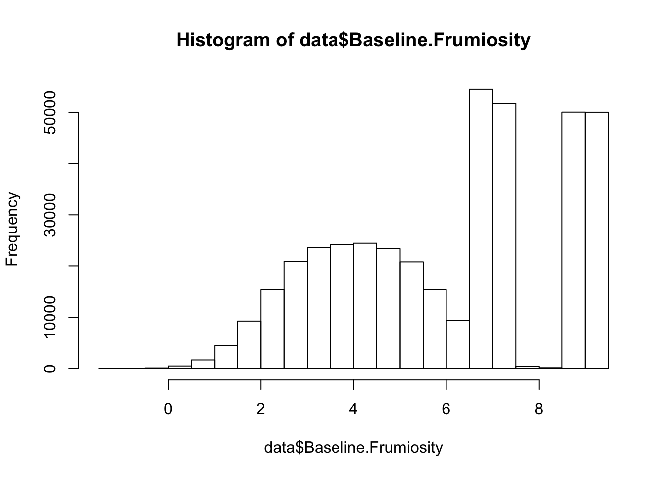
| Version | Author | Date |
|---|---|---|
| dd1e411 | Anthony Hung | 2019-05-22 |
hist(data$Post.Frumiosity)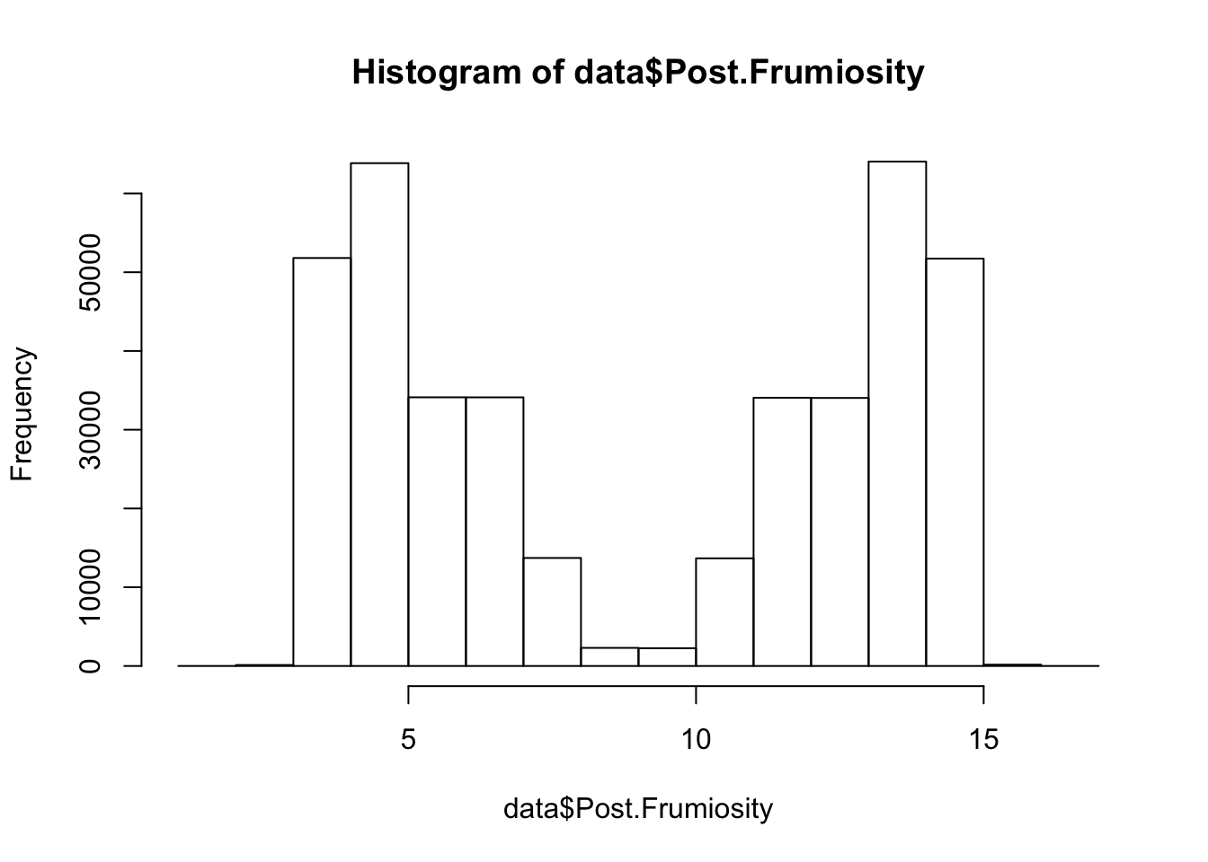
| Version | Author | Date |
|---|---|---|
| dd1e411 | Anthony Hung | 2019-05-22 |
plot(data$Baseline.Frumiosity, data$Post.Frumiosity)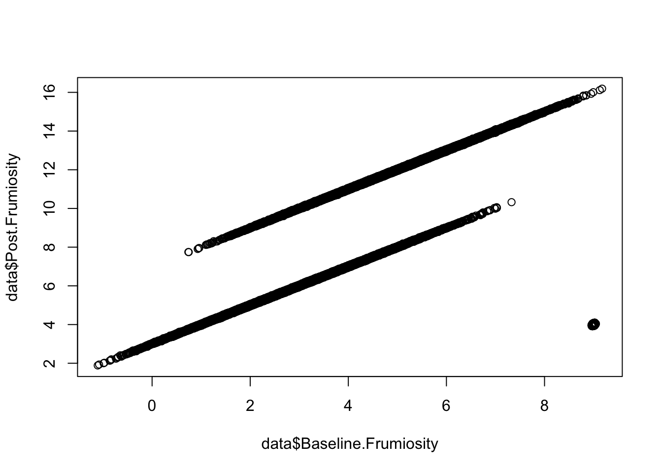
| Version | Author | Date |
|---|---|---|
| dd1e411 | Anthony Hung | 2019-05-22 |
#we can also write data files and export them using R
data$Size <- rnorm(nrow(data))
write.csv(data, "~/Desktop/data/new_bandersnatch.csv")
Exercises:
Write a function called calc_KE that takes as arguments the mass (in kg) and velocity (in m/s) of an object and returns the kinetic energy (in Joules) of an object. Use it to find the KE of a 0.5 kg rock moving at 1.2 m/s.
0.36 Joules Working with the gapminder dataset, find the country with the highest life expectancy in 1962.
Iceland Based on the plots we made of the bandersnatch data, there seems to be something going on that could potentially be interesting. Find out what might explain the structure in the data we see.
sessionInfo()R version 3.5.1 (2018-07-02)
Platform: x86_64-apple-darwin15.6.0 (64-bit)
Running under: macOS 10.14.5
Matrix products: default
BLAS: /Library/Frameworks/R.framework/Versions/3.5/Resources/lib/libRblas.0.dylib
LAPACK: /Library/Frameworks/R.framework/Versions/3.5/Resources/lib/libRlapack.dylib
locale:
[1] en_US.UTF-8/en_US.UTF-8/en_US.UTF-8/C/en_US.UTF-8/en_US.UTF-8
attached base packages:
[1] stats graphics grDevices utils datasets methods base
other attached packages:
[1] gapminder_0.3.0
loaded via a namespace (and not attached):
[1] Rcpp_0.12.18 knitr_1.20 whisker_0.3-2 magrittr_1.5
[5] workflowr_1.3.0 rlang_0.2.2 fansi_0.3.0 stringr_1.3.1
[9] tools_3.5.1 utf8_1.1.4 cli_1.0.0 git2r_0.23.0
[13] htmltools_0.3.6 yaml_2.2.0 rprojroot_1.3-2 digest_0.6.16
[17] assertthat_0.2.1 tibble_1.4.2 crayon_1.3.4 fs_1.2.7
[21] glue_1.3.0 evaluate_0.11 rmarkdown_1.10 stringi_1.2.4
[25] compiler_3.5.1 pillar_1.3.0 backports_1.1.2