Lipid 711
borangao
2023-10-09
Last updated: 2023-10-09
Checks: 7 0
Knit directory: meSuSie_Analysis/
This reproducible R Markdown analysis was created with workflowr (version 1.7.0). The Checks tab describes the reproducibility checks that were applied when the results were created. The Past versions tab lists the development history.
Great! Since the R Markdown file has been committed to the Git repository, you know the exact version of the code that produced these results.
Great job! The global environment was empty. Objects defined in the global environment can affect the analysis in your R Markdown file in unknown ways. For reproduciblity it’s best to always run the code in an empty environment.
The command set.seed(20220530) was run prior to running
the code in the R Markdown file. Setting a seed ensures that any results
that rely on randomness, e.g. subsampling or permutations, are
reproducible.
Great job! Recording the operating system, R version, and package versions is critical for reproducibility.
Nice! There were no cached chunks for this analysis, so you can be confident that you successfully produced the results during this run.
Great job! Using relative paths to the files within your workflowr project makes it easier to run your code on other machines.
Great! You are using Git for version control. Tracking code development and connecting the code version to the results is critical for reproducibility.
The results in this page were generated with repository version 62ce4b3. See the Past versions tab to see a history of the changes made to the R Markdown and HTML files.
Note that you need to be careful to ensure that all relevant files for
the analysis have been committed to Git prior to generating the results
(you can use wflow_publish or
wflow_git_commit). workflowr only checks the R Markdown
file, but you know if there are other scripts or data files that it
depends on. Below is the status of the Git repository when the results
were generated:
Untracked files:
    Untracked:  data/GLGC_chr_22.txt
    Untracked:  data/MESuSiE_Example.RData
    Untracked:  data/UKBB_chr_22.txt

Unstaged changes:
    Modified:   analysis/_site.yml
    Modified:   analysis/about.Rmd
    Deleted:    analysis/illustration.Rmd
    Deleted:    analysis/toy_example.Rmd
Note that any generated files, e.g. HTML, png, CSS, etc., are not included in this status report because it is ok for generated content to have uncommitted changes.
These are the previous versions of the repository in which changes were
made to the R Markdown (analysis/Lipid_711.Rmd) and HTML
(docs/Lipid_711.html) files. If you’ve configured a remote
Git repository (see ?wflow_git_remote), click on the
hyperlinks in the table below to view the files as they were in that
past version.
| File | Version | Author | Date | Message |
|---|---|---|---|---|
| Rmd | 62ce4b3 | borangao | 2023-10-09 | Update my analysis |
711 Regions of 4 lipid traits
Note: all the code and analysis reproduced here can be found in Zenodo
1. Feature of 95% credible set
1a. Set size and eQTL enrichment of 95% credible set
library(ggpubr)
library(data.table)
library(dplyr)
library(tidyr)
library(ggplot2)
library(patchwork)
library(ggpmisc)
library(VennDiagram)
library(gridExtra)
library(ggbreak)
library(DescTools)
library(coin)
library(susieR)
library(ggrepel)
library(stringr)


load("/net/fantasia/home/borang/Susie_Mult/Revision_Round_1/01_06_Real_Data/summary_res/res.RData")
custom_theme <- function() {
  theme(
    axis.text.x = element_text(size = 5),
    axis.text.y = element_text(size = 5),
    axis.title.x = element_text(size = 7, face="bold"),
    axis.title.y = element_text(size = 7, face="bold"),
    strip.text.x = element_text(size = 5),
    strip.text.y = element_text(size = 5),
    strip.background = element_blank(),
    legend.text = element_text(size=7),
    legend.title = element_text(size=7, face="bold"),
    plot.title = element_text(size=7, hjust = 0.5),
    panel.grid.major = element_blank(),
    panel.grid.minor = element_blank(),
    panel.border = element_blank(),
    axis.line = element_line(color = "black")
  )
}
################################################
#
#       Set Size/Z-score/eQTL
#
#
###############################################
################################################
#
#       Set SiZe Part
#
###############################################
###Median set size by Trait
all_sets_info<-data.frame(res_all%>%group_by(Trait,Region) %>% summarise(across(c("MESuSiE_cs", "SuSiE_cs","Paintor_cs"), ~ sum(.x, na.rm = TRUE))))%>%filter(MESuSiE_cs!=0, SuSiE_cs!=0, Paintor_cs!=0) ###Median Set Size across all locus
all_sets_info_long<-all_sets_info%>%pivot_longer(!(Trait|Region), names_to = "Method", values_to = "Count")
all_sets_info_long$Method<-factor(all_sets_info_long$Method,levels=c("MESuSiE_cs","SuSiE_cs","Paintor_cs"))
levels(all_sets_info_long$Method)<-c("MESuSiE","SuSiE","Paintor")

p_set = ggplot(data =all_sets_info_long,aes(x = Trait, y=Count,fill=Method))+geom_boxplot(aes(x = Trait,fill=Method),outlier.size = 0.1,fatten = 0.5,color = "darkgray")+scale_fill_manual(values=c("MESuSiE"="#023e8a","SuSiE"="#2a9d8f","Paintor"="#f4a261"),guide=FALSE)
p_set =p_set + theme_bw() + xlab("") +ylab("Set Size")+coord_cartesian(ylim=c(0,175))
p_set= p_set+custom_theme()

################################################
#
#       Z-score Part
#
###############################################
MESuSiE_cs_Z<-res_all%>%group_by(Trait) %>%filter(MESuSiE_cs==1)%>%summarise(zmax = median(pmax(abs(zscore_WB),abs(zscore_BB))))
SuSiE_cs_Z<-res_all%>%group_by(Trait) %>%filter(SuSiE_cs==1)%>%summarise(zmax =median(pmax(abs(zscore_WB),abs(zscore_BB))))%>%pull(zmax)
Paintor_cs_Z<-res_all%>%group_by(Trait) %>%filter(Paintor_cs==1)%>%summarise(zmax = median(pmax(abs(zscore_WB),abs(zscore_BB))))%>%pull(zmax)
set_size_z_info<-data.frame(cbind(MESuSiE_cs_Z,SuSiE_cs_Z,Paintor_cs_Z))
colnames(set_size_z_info)<-c("Trait",c("MESuSiE","SuSiE","Paintor"))
set_size_z_info_long<-set_size_z_info %>%pivot_longer(!(Trait), names_to = "Method", values_to = "Z")%>%mutate(Method = factor(Method, levels=c("MESuSiE","SuSiE","Paintor")))

p_z = ggplot(data = set_size_z_info_long,aes(x = Trait, y=Z,fill=Method))+geom_bar( stat = "identity",position="dodge")+scale_fill_manual(values=c("MESuSiE"="#023e8a","SuSiE"="#2a9d8f","Paintor"="#f4a261"))
p_z = p_z + geom_text(label = round(set_size_z_info_long$Z,2),position = position_dodge(width = 1),vjust=-0.5,size = 5*5/14)
p_z = p_z + theme_bw() + xlab("") +ylab("Median |Z|")+ ylim(0,max(round(set_size_z_info_long$Z,2)+1))
p_z = p_z +custom_theme()
################################################
#
#       eQTL enrichment
#
#
###############################################
 ann_col_name<-c("missense", "synonymous", "utr_comb", "promotor", "CRE","liver_ind_eQTL")
  # Functions for calculating fold enrichment
  calc_fold_enrichment <- function(df, cs_col, ann_col_name) {
    df %>%
      group_by(Region) %>%
      filter(sum(!!sym(cs_col)) != 0) %>%
      group_by(Trait, !!sym(cs_col)) %>%
      summarise(across(ann_col_name, ~ sum(.x, na.rm = TRUE) / n())) %>%
      group_by(Trait) %>%
      summarise(across(ann_col_name, ~ .x[!!sym(cs_col) == 1] / .x[!!sym(cs_col) == 0]))
  }

  MESuSiE_PIP_ann <- calc_fold_enrichment(res_all, "MESuSiE_cs", ann_col_name)
  SuSiE_PIP_ann <- calc_fold_enrichment(res_all, "SuSiE_cs", ann_col_name)
  Paintor_PIP_ann <- calc_fold_enrichment(res_all, "Paintor_cs", ann_col_name)
  # Combine results
  Trait_CS_enrichment <- bind_rows(
    MESuSiE_PIP_ann %>% mutate(Method = "MESuSiE"),
    SuSiE_PIP_ann %>% mutate(Method = "SuSiE"),
    Paintor_PIP_ann %>% mutate(Method = "Paintor")
  ) %>% mutate(Method = factor(Method, levels = c("MESuSiE", "SuSiE", "Paintor")))%>%
    dplyr::select(Trait,liver_ind_eQTL ,Method )%>%dplyr::rename(eQTL = liver_ind_eQTL)
  # Pivot to long format
  Trait_CS_enrichment_long <- Trait_CS_enrichment %>%
    pivot_longer(cols = -c(Method, Trait), names_to = "Cat", values_to = "Prop") %>%
    mutate(Method = factor(Method, levels = c("MESuSiE", "SuSiE", "Paintor")))

p_eQTL <- ggplot(Trait_CS_enrichment_long, aes(x = Trait, y = Prop, fill = Method)) +
  geom_bar(stat = "identity", position = "dodge") +scale_fill_manual(values = c("MESuSiE" = "#023e8a", "SuSiE" = "#2a9d8f", "Paintor" = "#f4a261")) +
  geom_text(,label = round(Trait_CS_enrichment_long$Prop,2),position = position_dodge(width = 1),vjust=-0.5,size = 5*5/14)+
  xlab("") + ylab("eQTL Fold Enrichment") + ylim(0,max(round(Trait_CS_enrichment_long$Prop))+1)+
  theme_bw() + custom_theme()

p_out<-p_set/p_z/p_eQTL+plot_annotation(tag_levels = 'a')+plot_layout(guides = "collect",heights = c(1.5,1,1))&theme(legend.position = 'bottom',plot.tag = element_text(size = 7,face="bold"))
p_out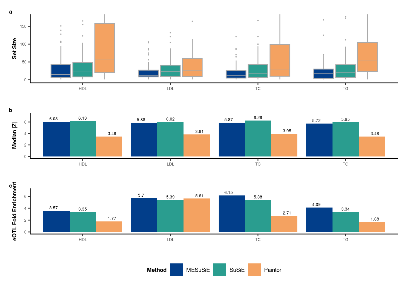
1b. Functional enrichment of 95% credible set and top signals
################################################################################
#
#
#     Functional Annotation enrichment for 95% credible set SNPS
#
#
################################################################################
 # Enrichment of 95% credible set without by trait
  calc_fold_enrichment_marginal<-function(df, cs_col, ann_col_name) {
    df %>%group_by(Region) %>%
      filter(sum(!!sym(cs_col)) != 0) %>%
      group_by( !!sym(cs_col)) %>%
      summarise(across(ann_col_name, ~ sum(.x, na.rm = TRUE) / n())) %>%
      summarise(across(ann_col_name, ~ .x[!!sym(cs_col) == 1] / .x[!!sym(cs_col) == 0]))
  }
  MESuSiE_PIP_ann <- calc_fold_enrichment_marginal(res_all, "MESuSiE_cs", ann_col_name)
  SuSiE_PIP_ann <- calc_fold_enrichment_marginal(res_all, "SuSiE_cs", ann_col_name)
  Paintor_PIP_ann <- calc_fold_enrichment_marginal(res_all, "Paintor_cs", ann_col_name)

  CS_enrichment <- bind_rows(
    MESuSiE_PIP_ann %>% mutate(Method = "MESuSiE"),
    SuSiE_PIP_ann %>% mutate(Method = "SuSiE"),
    Paintor_PIP_ann %>% mutate(Method = "Paintor")
  ) %>% mutate(Method = factor(Method, levels = c("MESuSiE", "SuSiE", "Paintor")))%>%
    dplyr::rename(Missense = missense ,Synonymous = synonymous,UTR = utr_comb,Promotor = promotor,eQTL = liver_ind_eQTL)

  # Pivot to long format
  CS_enrichment_long <- CS_enrichment %>%
    pivot_longer(cols = -c(Method), names_to = "Cat", values_to = "Prop") %>%
    mutate(Method = factor(Method, levels = c("MESuSiE", "SuSiE", "Paintor"))) %>%
    mutate(Cat = factor(Cat, levels = c("Missense", "Synonymous", "UTR", "Promotor", "CRE","eQTL")))%>%
    mutate(Prop = round(Prop, 2))

p_set <- ggplot(data = CS_enrichment_long,aes(x = Cat, y = Prop, fill = Method)) +
  geom_col(position = "dodge") + scale_fill_manual(values = c("MESuSiE" = "#023e8a", "SuSiE" = "#2a9d8f", "Paintor" = "#f4a261")) +
  geom_text(aes(x=Cat,group=Method,y=Prop,label=Prop),position = position_dodge(width = 1),vjust=-0.5,size = 5/14*5) +
  geom_hline(yintercept = 1, linetype = "dashed") +
  xlab("") + ylab("Fold Enrichment Credible Set") +ylim(0,round(max(CS_enrichment_long$Prop))+1) +
  theme_bw() + custom_theme()
################################################################################
#
#
#     Functional Annotation enrichment for top 500 PIP SNPs
#
#
################################################################################
  # Enrichment of top 500 signal
  res_all<-res_all%>%mutate(Paintor_Signal = ifelse(Paintor_PIP>0.5,1,0))
  res_all<-res_all%>%mutate(SuSiE_Signal = case_when(
    SuSiE_WB>0.5&SuSiE_BB>0.5~1,
    SuSiE_WB>0.5&SuSiE_BB<0.5~2,
    SuSiE_WB<0.5&SuSiE_BB>0.5~3,
    .default =0))
  res_all<-res_all%>%mutate(MESuSiE_Signal = case_when(
    MESuSiE_PIP_Shared>0.5~1,
    MESuSiE_PIP_WB>0.5~2,
    MESuSiE_PIP_BB>0.5~3,
    .default =0))
  top_N_signal = 500
  bg_an<-res_all%>%summarise(across(ann_col_name,~ sum(.x, na.rm = TRUE)/n()))
  MESuSiE_Signal_ann<-res_all%>%filter(MESuSiE_Signal!=0)%>% arrange(desc(MESuSiE_PIP_Either))%>%top_n(n = top_N_signal, wt = MESuSiE_PIP_Either)%>%summarise(across(ann_col_name,~ sum(.x, na.rm = TRUE)/n()))/bg_an
  SuSiE_Signal_ann<-res_all%>%filter(SuSiE_Signal!=0)%>% arrange(desc(SuSiE_PIP))%>%top_n(n = top_N_signal, wt = SuSiE_PIP)%>%summarise(across(ann_col_name,~ sum(.x, na.rm = TRUE)/n()))/bg_an
  Paintor_Signal_ann<-res_all%>%filter(Paintor_Signal!=0) %>% arrange(desc(Paintor_PIP))%>%top_n(n = top_N_signal, wt = Paintor_PIP)%>%summarise(across(ann_col_name,~ sum(.x, na.rm = TRUE)/n()))/bg_an

  Signal_enrichment <- bind_rows(
    MESuSiE_Signal_ann %>% mutate(Method = "MESuSiE"),
    SuSiE_Signal_ann %>% mutate(Method = "SuSiE"),
    Paintor_Signal_ann %>% mutate(Method = "Paintor")
  ) %>% mutate(Method = factor(Method, levels = c("MESuSiE", "SuSiE", "Paintor")))%>%
    dplyr::rename(Missense = missense ,Synonymous = synonymous,UTR = utr_comb,Promotor = promotor,eQTL = liver_ind_eQTL)
  # Pivot to long format
  Signal_enrichment_long <- Signal_enrichment %>%
    pivot_longer(cols = -c(Method), names_to = "Cat", values_to = "Prop") %>%
    mutate(Method = factor(Method, levels = c("MESuSiE", "SuSiE", "Paintor"))) %>%
    mutate(Cat = factor(Cat, levels = c("Missense", "Synonymous", "UTR", "Promotor", "CRE","eQTL")))%>%
    mutate(Prop = round(Prop, 2))

p_signal <- ggplot(data = Signal_enrichment_long,aes(x = Cat, y = Prop, fill = Method)) +
  geom_col(position = "dodge") + scale_fill_manual(values = c("MESuSiE" = "#023e8a", "SuSiE" = "#2a9d8f", "Paintor" = "#f4a261")) +
  geom_text(aes(x=Cat,group=Method,y=Prop,label=Prop),position = position_dodge(width = 1),vjust=-0.5,size = 5/14*5) +
  geom_hline(yintercept = 1, linetype = "dashed") +
  xlab("") + ylab("Fold Enrichment Top Signal") +ylim(0,round(max(Signal_enrichment_long$Prop))+1) +
  theme_bw() + custom_theme()
p_out<-p_set/p_signal+plot_annotation(tag_levels = 'a')+plot_layout(guides = "collect",heights = c(1,1))&theme(legend.position = 'bottom',plot.tag = element_text(size = 7,face="bold"))
p_out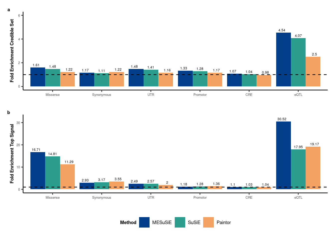
2. Top signals with PIP > 0.5
2a. Proportion of shared and ancestry-specific signal
############################################################################
#
#
#              Proportion of Signal Plot
#
#
############################################################################
Signal_number<- res_all%>%group_by(Trait)%>%
  summarise(Paintor_Either_n = sum(Paintor_Signal!=0),
            SuSiE_Shared_n = sum(SuSiE_Signal==1),
            SuSiE_WB_n = sum(SuSiE_Signal==2),
            SuSiE_BB_n = sum(SuSiE_Signal==3),
            MESuSiE_Shared_n = sum(MESuSiE_Signal==1),
            MESuSiE_WB_n = sum(MESuSiE_Signal==2),
            MESuSiE_BB_n = sum(MESuSiE_Signal==3))
Signal_number<-Signal_number%>%
  pivot_longer(cols = -c(Trait), names_to = "Cat", values_to = "Num")%>%
  separate(Cat, into = c("Method", "Signal"), sep = "_", extra = "merge") %>%
  mutate(
    Method = case_when(
      str_detect(Method, "MESuSiE") ~ "MESuSiE",
      str_detect(Method, "SuSiE") ~ "SuSiE",
      str_detect(Method, "Paintor") ~ "Paintor",
      TRUE ~ Method
    ),
    Signal = case_when(
      str_detect(Signal, "BB_n") ~ "AFR",
      str_detect(Signal, "WB_n") ~ "EUR",
      str_detect(Signal, "Shared_n") ~ "Shared",
      str_detect(Signal, "Either") ~ "Either",
      TRUE ~ Signal
    )
  )
Signal_number<-Signal_number%>%group_by(Method,Trait)%>%mutate(prop = Num/sum(Num)*100,ypos = cumsum(prop)- 0.5*prop)%>%mutate(label = paste0(Signal," ",Num))
Signal_number<-Signal_number%>%mutate(Method = factor(Method, levels = c("MESuSiE","SuSiE","Paintor")),Signal = factor(Signal, levels = c("EUR","AFR","Shared","Either")))

signal_num_plot<-ggplot(Signal_number, aes(x="", y=prop, fill=Signal)) +
  geom_bar(stat="identity", width=1, color="white") +
  coord_polar("y", start=0) +
  theme_void() +
  theme(legend.position="none") +
  geom_text(aes(y = ypos, label = label),  size=7/14*5,color="white") +
  scale_fill_manual(values=c("#ABDB9F","#F2C1B6","#6162B0","gray"))+
  facet_grid(vars(Trait),vars(Method),labeller=label_parsed)+theme(
    strip.text.x = element_text(size = 7,face="bold"),
    strip.text.y = element_text(size = 7,face="bold"),
    strip.background = element_blank(),
    panel.grid.major = element_blank(),
    panel.grid.minor = element_blank(),
    panel.border = element_blank())
signal_num_plot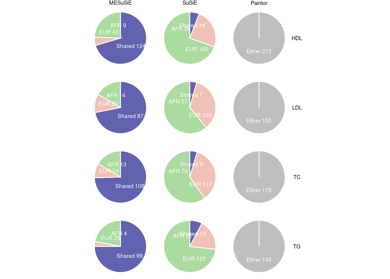
2b. Feature of shared and ancestry-specific signal
###########################################################################################
#
#
#         Correlation of ancestry-specific signal by MESuSiE and SuSiE
#
#
#########################################################################################
cor_ancestry_MESuSiE <- res_all %>%
    filter(MESuSiE_Signal%in%c(2,3)) %>% filter(!(SuSiE_Signal%in%c(2,3)))%>%
    mutate(Method = "MESuSiE") %>%
    dplyr::select(Beta_WB, Beta_BB, Trait, Method)
  cor_ancestry_SuSiE <- res_all %>%
    filter(SuSiE_Signal%in%c(2,3)) %>%filter(!(MESuSiE_Signal%in%c(2,3)))%>%
    mutate(Method = "SuSiE") %>%
    dplyr::select(Beta_WB, Beta_BB, Trait, Method)
  cor_ancestry_both <- res_all %>%filter(MESuSiE_Signal%in%c(2,3),SuSiE_Signal%in%c(2,3))%>%
    mutate(Method = "Both") %>%
    dplyr::select(Beta_WB, Beta_BB, Trait, Method)
  cor_ancestry <- rbind(cor_ancestry_MESuSiE, cor_ancestry_SuSiE,cor_ancestry_both)
  cor_ancestry<-cor_ancestry%>%mutate(Method = factor(Method,levels = c("MESuSiE","SuSiE","Both")))

betaplot<- ggscatter(cor_ancestry, x = "Beta_WB", y = "Beta_BB",
                add = "reg.line",  # Add regressin line
                add.params = list(color = "red", fill = "lightgray",size = 0.5), # Customize reg. line
                conf.int = FALSE, # Add confidence interval
                size = 0.5
)+ stat_cor(method = "pearson",aes(label = ..r.label..),size = 5/14*5)+xlab("UKBB")+ylab("GLGC")+
  theme_bw() + custom_theme()+
  facet_wrap(vars(Method),ncol=3)
betaplot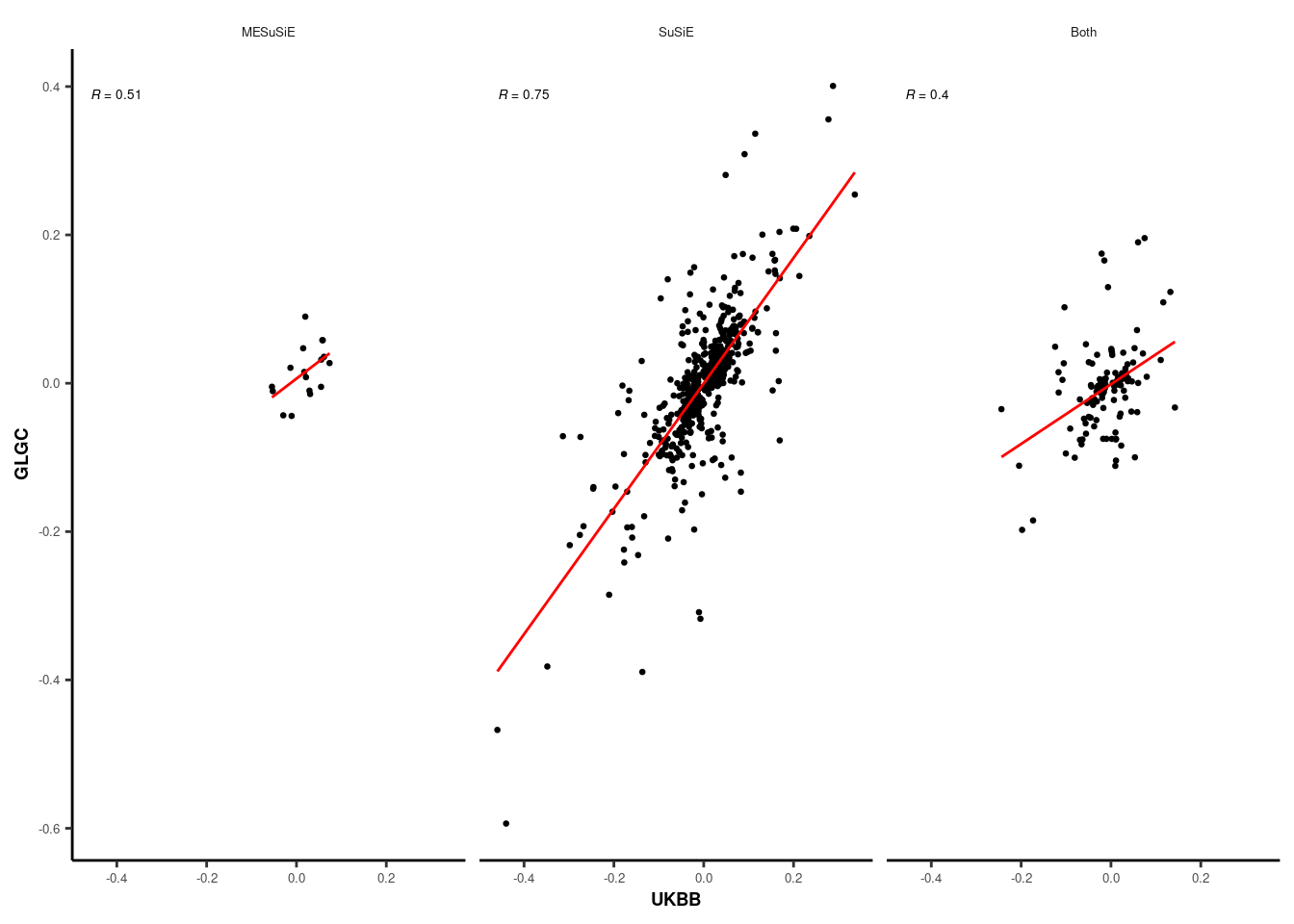
#################################################################
#
#
#               MAF and Conservative Score Part
#
#
##################################################################
################################################
#
#       Phylop/GERP Score Part
#
#
################################################

res_all<- res_all %>%
  mutate(
    MESuSiE_Conservative = case_when(
      MESuSiE_PIP_WB>0.5|MESuSiE_PIP_BB>0.5 ~ "Ancestry-specific",
      MESuSiE_PIP_Shared>0.5 ~ "Shared",
      TRUE ~ "None"
    ),
    SuSiE_Conservative = case_when(
      (SuSiE_WB>0.5&SuSiE_BB<0.5)|(SuSiE_BB>0.5&SuSiE_WB<0.5) ~ "Ancestry-specific",
      SuSiE_Shared>0.5 ~ "Shared",
      TRUE ~ "None"
    )
  )%>%
  mutate(
    MESuSiE_Conservative = factor(MESuSiE_Conservative, levels = c("None", "Ancestry-specific", "Shared")),
    SuSiE_Conservative = factor(SuSiE_Conservative, levels = c("None", "Ancestry-specific", "Shared"))
  )


####Phylop
grouped_data_phylop <- res_all %>%
  mutate(abs_phylop = abs(phylop)) %>%
  select(MESuSiE_Conservative, abs_phylop)%>%
  group_by(MESuSiE_Conservative) %>%
  summarise(phylop_values = list(abs_phylop))%>%
  pull(phylop_values)


grouped_data_GERP <- res_all %>%
  mutate(GERP = abs(GERP)) %>%
  select(MESuSiE_Conservative, GERP)%>%
  group_by(MESuSiE_Conservative) %>%
  summarise(GERP_values = list(GERP))%>%
  pull(GERP_values)


#########Conservation Plot
conserve_data<-res_all%>%mutate(Signal =MESuSiE_Conservative, Phylop =abs(phylop) )%>%select(Signal,Phylop,GERP)
conserve_data_long<-conserve_data%>%pivot_longer(!(Signal), names_to = "Method", values_to = "Score")
conserve_data_long$Method<-factor(conserve_data_long$Method,levels = c("Phylop","GERP"))
df <-conserve_data_long %>%group_by(Method,Signal) %>%summarize(ymin = min(Score,na.rm = T), lower = quantile(Score, .25,na.rm = T),  middle = mean(Score,na.rm = T), upper = quantile(Score, .75,na.rm = T),ymax = max(Score,na.rm = T))
p_set_phylop = df %>% ggplot(aes(x = factor(Method), fill=Signal)) + geom_boxplot(fatten = 2,aes(ymin = ymin, ymax = ymax, lower = lower, upper = upper, middle = middle), stat = 'identity')+scale_fill_manual(values=c("None"="#DAFFED","Ancestry-specific"="#fffbdb","Shared" = "#7776bc"))
p_set_phylop =p_set_phylop + theme_bw() + xlab("") +ylab("Conservation Score")
p_set_phylop= p_set_phylop  + custom_theme()
p_set_phylop= p_set_phylop+ theme(legend.position="bottom")

################################################
#
#       MAF Part
#
#
################################################
 maf_shared<-data.frame(res_all)%>%filter(MESuSiE_Signal==1)%>%mutate(MAF_diff = ifelse(MA_WB==MA_BB,MAF_WB-MAF_BB,1-MAF_WB-MAF_BB))%>%pull(MAF_diff)
  maf_ancestry<-data.frame(res_all)%>%filter(MESuSiE_Signal%in%c(2,3))%>%mutate(MAF_diff = ifelse(MA_WB==MA_BB,MAF_WB-MAF_BB,1-MAF_WB-MAF_BB))%>%pull(MAF_diff)


maf_data_plot<-data.frame("MAF" = c(maf_shared,maf_ancestry),"Signal"=c(rep("Shared",length(maf_shared)),rep("Ancestry-specific",length(maf_ancestry))))
maf_data_plot$Signal<-factor(maf_data_plot$Signal)
maf_data_plot$Signal<-factor(maf_data_plot$Signal,levels = c(levels(maf_data_plot$Signal),"None"))

p_set = ggplot(data =maf_data_plot,aes(x = factor(Signal), y=MAF,fill=Signal))+geom_boxplot(aes(x = factor(Signal),fill=Signal),outlier.size = 0.01) +scale_fill_manual(values=c("None"="#DAFFED","Ancestry-specific"="#fffbdb","Shared" = "#7776bc"),guide=FALSE)
p_set = p_set + stat_compare_means(size= 5/14*5)
p_set =p_set + theme_bw() + xlab("") +ylab("MAF difference")
p_set= p_set + custom_theme()
p_set= p_set + theme(legend.position="none")
p_out<-p_set+p_set_phylop+plot_annotation(tag_levels = 'a') + plot_layout(guides = "collect") & theme(legend.position = "bottom",plot.tag = element_text(size = 7,face="bold"))
p_out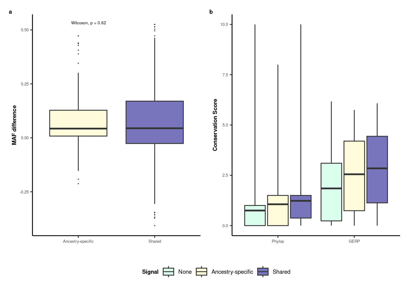
3. Example locus
3a. FAD2 Example
##############################################################
#
#
#       Real Data Example Plotter
#
#
################################################################

gwas_plot_fun <- function(data_plot, xlab_name, ylab_name, yintercept) {

  p_manhattan = ggplot() + geom_point(data = data_plot%>%filter(Lead_SNP==0), aes(x = POS, y = PIP, color = r2), size = 1)
  p_manhattan = p_manhattan + geom_point(data = data_plot%>%filter(Lead_SNP==1), aes(x = POS, y = PIP), size = 1.5, color = "red") +
    geom_text_repel(data = data_plot%>%filter(Lead_SNP==1), mapping = aes(x = POS, y = PIP, label = SNP), vjust = 1.2, size = 7/14*5, show.legend =FALSE)
  p_manhattan = p_manhattan +
    scale_color_stepsn(
      colors = c("navy", "lightskyblue", "green", "orange", "red"),
      breaks = seq(0.2, 0.8, by = 0.2),
      limits = c(0, 1),
      show.limits = TRUE,
      na.value = 'grey50',
      name = expression(R^2)
    )
  p_manhattan = p_manhattan +
    geom_hline(
      yintercept = yintercept,
      linetype = "dashed",
      color = "grey50",
      size = 0.5
    )
  p_manhattan = p_manhattan +
    geom_vline(
      xintercept = data_plot%>%filter(lead_SNP==1)%>%pull(POS),
      linetype = "dashed",
      color = "grey50",
      size = 0.5
    )
  p_manhattan = p_manhattan + xlim(min(data_plot$POS),max(data_plot$POS))
  p_manhattan = p_manhattan + expand_limits(x = round(max(data_plot$POS)/1e6)*1e6)
  if(max(data_plot$POS>1e6)){
    p_manhattan = p_manhattan + scale_x_continuous(labels = function(x) paste0(x / 1e6, " MB"))
  }
  if(max(data_plot$POS<1e6)){
    p_manhattan = p_manhattan + scale_x_continuous(labels = function(x) paste0(x / 1e3, " KB"))
  }
  p_manhattan = p_manhattan + xlab(xlab_name) +ylab(ylab_name)
  p_manhattan = p_manhattan + guides(fill = guide_legend(title = as.expression(bquote(R^2))))
  p_manhattan = p_manhattan + theme_bw()+custom_theme()
  return(p_manhattan)
}

###Function used for PIP plot
finemap_plot_fun<-function(data_plot,xlab_name,ylab_name,yintercept){
  p_manhattan = ggplot() + geom_point(data = data_plot, aes(x = POS, y = PIP, color = r2,shape = cat))+scale_shape_manual(name="Category",drop=FALSE,values=c(20,24,25,23,22))
  p_manhattan = p_manhattan + geom_text_repel(data =data_plot%>%filter(Lead_SNP==1), mapping=aes(x=POS, y=PIP, label=SNP),vjust=1.2, size= 7/14*5,show.legend = FALSE)
  p_manhattan = p_manhattan + theme_bw()+scale_color_stepsn(
    colors = c("navy", "lightskyblue", "green", "orange", "red"),
    breaks = seq(0.2, 0.8, by = 0.2),
    limits = c(0, 1),
    show.limits = TRUE,
    na.value = 'grey50',
    name = expression(R^2)
  )
  p_manhattan = p_manhattan + geom_hline(
    yintercept =yintercept,
    linetype = "dashed",
    color = "grey50",
    size = 0.5
  ) + geom_vline(
    xintercept = data_plot%>%filter(lead_SNP==1)%>%pull(POS),
    linetype = "dashed",
    color = "grey50",
    size = 0.5
  )
  p_manhattan = p_manhattan + xlim(min(data_plot$POS),max(data_plot$POS))
  p_manhattan = p_manhattan + expand_limits(x = round(max(data_plot$POS)/1e6)*1e6)
  if(max(data_plot$POS>1e6)){
    p_manhattan = p_manhattan + scale_x_continuous(labels = function(x) paste0(x / 1e6, " MB"))
  }
  if(max(data_plot$POS<1e6)){
    p_manhattan = p_manhattan + scale_x_continuous(labels = function(x) paste0(x / 1e3, " KB"))
  }
  p_manhattan= p_manhattan+xlab(xlab_name)+ylab(ylab_name)
  p_manhattan= p_manhattan+guides(fill=guide_legend(title=as.expression(bquote(R^2))))
  p_manhattan = p_manhattan + theme_bw()+custom_theme()
  return(p_manhattan)
}
# Function used for gene plot
gene_range_plot_fun<-function(gene_list_data,plot.range){
  p<-ggplot(data = gene_list_data) +
    geom_linerange(aes(x = Gene, ymin = Start, ymax = End))+ylim(plot.range)+ expand_limits(y = round(max(plot.range[2])/1e6)*1e6)+scale_y_continuous(labels = function(y) paste0(y / 1e6, " MB"))+coord_flip()+
    geom_text(aes(x = Gene, y = Start, label = Gene), hjust = "right", size = 5/14*5) + ylab(paste0("chr",unique(gsub("chr","",gene_list_data$Chrom))))+ xlab("Gene") +
    theme_bw() +  theme(
      axis.text.x = element_text(size = 5),
      axis.text.y = element_blank(),
      axis.ticks.y =  element_blank(),
      axis.title.x = element_text(size = 7, face="bold"),
      axis.title.y = element_text(size = 7, face="bold"),
      strip.text.x = element_text(size = 5),
      strip.text.y = element_text(size = 5),
      strip.background = element_blank(),
      legend.text = element_text(size=7),
      legend.title = element_text(size=7, face="bold"),
      plot.title = element_text(size=7, hjust = 0.5),
      panel.grid.major = element_blank(),
      panel.grid.minor = element_blank(),
      panel.border = element_blank(),
      axis.line.x  = element_line(color = "black"),
      axis.line.y  = element_line(color = "black")
    )
  return(p)
}

#####################################################################################################################
#
#
#
#                 Example showcase
#
#
#
#####################################################################################################################
Gene_List<-fread("/net/fantasia/home/borang/Susie_Mult/simulation/simu_0120/data/Gencode_GRCh37_Genes_UniqueList2021.txt",header=T)

###################################################################
#
#
#             FADS2 independent eQTL shared signal
#
#
##################################################################
region = 384
trait_name = "TG"
ref_panel = "UKB1"
p_threshold_index = 1
res_z_dir<-paste0("/net/fantasia/home/borang/Susie_Mult/Revision_Round_1/01_02_Real_Data/",trait_name,"/",trait_name,"_REF_",ref_panel,"_P",p_threshold_index,"/")
out_dir<-paste0(res_z_dir,"data/")
out_res_dir<-paste0(res_z_dir,"res/")

##Data Reprocess
WB_COV<-as.matrix(fread(paste0(out_dir,"Region_",region,".LD1")))
BB_COV<-as.matrix(fread(paste0(out_dir,"Region_",region,".LD2")))
load(paste0(out_res_dir,"MESuSiE_region_",region,".RData"))

candidate_region<-res_all%>%filter(Region==region)
# rs174564 is the eQTL of FADS2 gene, highlighted in the paper
lead_SNP = "rs174564"
lead_SNP_index<-which(candidate_region$SNP==lead_SNP)
candidate_region<-candidate_region%>%mutate(r2_EUR  = unname(unlist((WB_COV[,lead_SNP_index])^2)) ,r2_AFR = unname(unlist((BB_COV[,lead_SNP_index])^2)),POS = as.numeric(POS))
####Category Setting
candidate_region<-candidate_region%>%mutate(SuSiE_cat = case_when(SuSiE_WB>0.5&SuSiE_BB>0.5 ~ 3,
                                                                  SuSiE_WB>0.5&SuSiE_BB<0.5 ~ 1,
                                                                  SuSiE_WB<0.5&SuSiE_BB>0.5 ~ 2,
                                                                  TRUE ~ 0),
                                            Paintor_cat = case_when(Paintor_PIP>0.5~4,
                                                                    TRUE~0),
                                            MESuSiE_cat = case_when(MESuSiE_PIP_WB>0.5~1,
                                                                    MESuSiE_PIP_BB>0.5~2,
                                                                    MESuSiE_PIP_Shared>0.5~3,
                                                                    TRUE~0))


###GWAS PLOT
EUR_GWAS_plot_data<-candidate_region%>%mutate(r2 = r2_EUR,PIP = -log10(2*pnorm(-abs(zscore_WB))),Lead_SNP = ifelse(SNP==lead_SNP,1,0),POS= as.numeric(POS))%>%select(SNP,POS, r2,PIP,Lead_SNP)
AFR_GWAS_plot_data<-candidate_region%>%mutate(r2 = r2_AFR,PIP = -log10(2*pnorm(-abs(zscore_BB))),Lead_SNP = ifelse(SNP==lead_SNP,1,0),POS= as.numeric(POS))%>%select(SNP,POS, r2,PIP,Lead_SNP)
p_EUR<-gwas_plot_fun (EUR_GWAS_plot_data, "UKBB", "-log10(P-value)", -log10(5e-8))
p_AFR<-gwas_plot_fun (AFR_GWAS_plot_data, "GLGC", "-log10(P-value)", -log10(5e-8))

###Finemap Plot
EUR_SuSiE_plot_data<-candidate_region%>%mutate(r2 = r2_EUR,PIP = SuSiE_WB,Lead_SNP = ifelse(SNP==lead_SNP,1,0),POS= as.numeric(POS),cat = factor(SuSiE_cat,levels = c("0", "1", "2", "3", "4"), labels = c("Non", "EUR", "AFR", "Shared", "Paintor")))%>%select(SNP,POS, r2,PIP,Lead_SNP,cat)
AFR_SuSiE_plot_data<-candidate_region%>%mutate(r2 = r2_AFR,PIP = SuSiE_BB,Lead_SNP = ifelse(SNP==lead_SNP,1,0),POS= as.numeric(POS),cat = factor(SuSiE_cat,levels = c("0", "1", "2", "3", "4"), labels = c("Non", "EUR", "AFR", "Shared", "Paintor")))%>%select(SNP,POS, r2,PIP,Lead_SNP,cat)
MESuSiE_plot_data<-candidate_region%>%mutate(r2 = r2_EUR,PIP = MESuSiE_PIP_Either,Lead_SNP = ifelse(SNP==lead_SNP,1,0),POS= as.numeric(POS),cat = factor(MESuSiE_cat,levels = c("0", "1", "2", "3", "4"), labels = c("Non", "EUR", "AFR", "Shared", "Paintor")))%>%select(SNP,POS, r2,PIP,Lead_SNP,cat)
Paintor_plot_data<-candidate_region%>%mutate(r2 = r2_EUR,PIP = Paintor_PIP,Lead_SNP = ifelse(SNP==lead_SNP,1,0),POS= as.numeric(POS),cat = factor(Paintor_cat,levels = c("0", "1", "2", "3", "4"), labels = c("Non", "EUR", "AFR", "Shared", "Paintor")))%>%select(SNP,POS, r2,PIP,Lead_SNP,cat)

p_EUR_SuSiE<-finemap_plot_fun(EUR_SuSiE_plot_data, "SuSiE UKBB", "PIP", 0.5)
p_AFR_SuSiE<-finemap_plot_fun(AFR_SuSiE_plot_data, "SuSiE GLGC", "PIP", 0.5)
p_MESuSiE<-finemap_plot_fun(MESuSiE_plot_data, "MESuSiE", "PIP", 0.5)
p_Paintor<-finemap_plot_fun(Paintor_plot_data, "Paintor", "PIP", 0.5)

# Gene Plot
plot.range <- c(min(candidate_region$POS), max(candidate_region$POS))
Gene_List_sub_coding<-Gene_List%>%filter(Chrom==paste0("chr",unique(candidate_region$CHR)))%>%filter(Start<max(candidate_region$POS),End>min(candidate_region$POS))%>%filter(Coding=="proteincoding")%>%filter(!is.na(cdsLength))%>%filter(GeneLength>15000)
p2<-gene_range_plot_fun(Gene_List_sub_coding,plot.range)

##Combine Plot together
combined_plot<-(p_EUR/p_EUR_SuSiE/p_MESuSiE/p2+plot_layout(heights = c(1,1,1,1.5))|p_AFR/p_AFR_SuSiE/p_Paintor/p2+plot_layout(heights = c(1,1,1,1.5)))+plot_layout(guides = 'collect')&theme(legend.position = "bottom")
combined_plot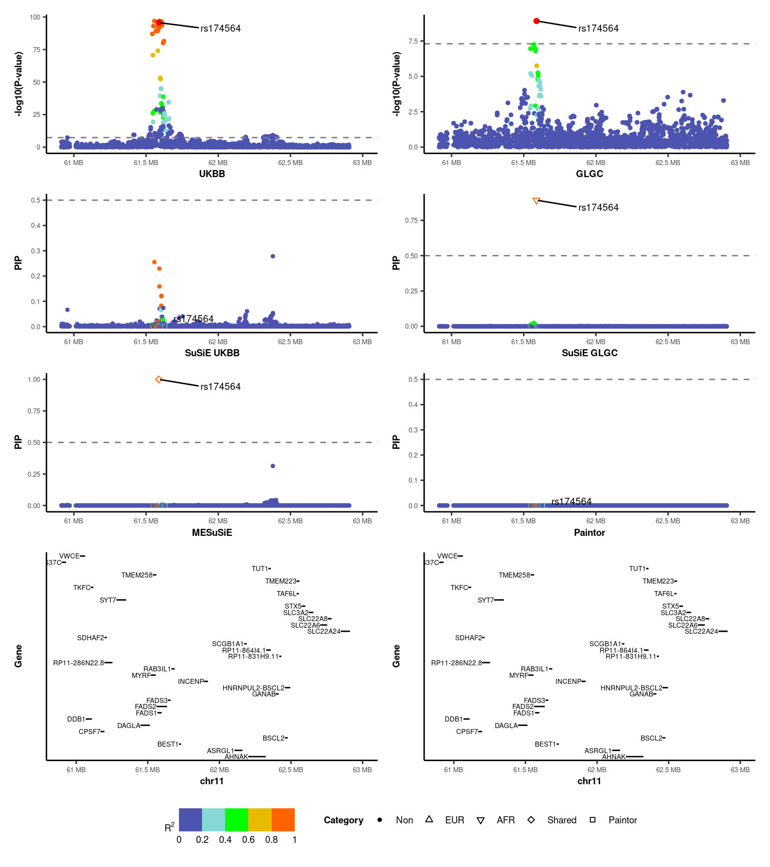
3b. APOH Example
##############################################################
#
#
#           APOH missense shared for TG (rs1801689)
#
################################################################
region = 438
trait_name = "TG"
ref_panel = "UKB1"
p_threshold_index = 1
res_z_dir<-paste0("/net/fantasia/home/borang/Susie_Mult/Revision_Round_1/01_02_Real_Data/",trait_name,"/",trait_name,"_REF_",ref_panel,"_P",p_threshold_index,"/")
out_dir<-paste0(res_z_dir,"data/")
out_res_dir<-paste0(res_z_dir,"res/")

##Date Reprocess
WB_COV<-as.matrix(fread(paste0(out_dir,"Region_",region,".LD1")))
BB_COV<-as.matrix(fread(paste0(out_dir,"Region_",region,".LD2")))
load(paste0(out_res_dir,"MESuSiE_region_",region,".RData"))

candidate_region<-res_all%>%filter(Region==region)
# rs1801689 is the missense of APOH gene, highlighted in the paper
lead_SNP = "rs1801689"
lead_SNP_index<-which(candidate_region$SNP==lead_SNP)
candidate_region<-candidate_region%>%mutate(r2_EUR  = unname(unlist((WB_COV[,lead_SNP_index])^2)) ,r2_AFR = unname(unlist((BB_COV[,lead_SNP_index])^2)),POS = as.numeric(POS))
####Category Setting
candidate_region<-candidate_region%>%mutate(SuSiE_cat = case_when(SuSiE_WB>0.5&SuSiE_BB>0.5 ~ 3,
                                                                  SuSiE_WB>0.5&SuSiE_BB<0.5 ~ 1,
                                                                  SuSiE_WB<0.5&SuSiE_BB>0.5 ~ 2,
                                                                  TRUE ~ 0),
                                            Paintor_cat = case_when(Paintor_PIP>0.5~4,
                                                                    TRUE~0),
                                            MESuSiE_cat = case_when(MESuSiE_PIP_WB>0.5~1,
                                                                    MESuSiE_PIP_BB>0.5~2,
                                                                    MESuSiE_PIP_Shared>0.5~3,
                                                                    TRUE~0))

###GWAS PLOT
EUR_GWAS_plot_data<-candidate_region%>%mutate(r2 = r2_EUR,PIP = -log10(2*pnorm(-abs(zscore_WB))),Lead_SNP = ifelse(SNP==lead_SNP,1,0),POS= as.numeric(POS))%>%select(SNP,POS, r2,PIP,Lead_SNP)
AFR_GWAS_plot_data<-candidate_region%>%mutate(r2 = r2_AFR,PIP = -log10(2*pnorm(-abs(zscore_BB))),Lead_SNP = ifelse(SNP==lead_SNP,1,0),POS= as.numeric(POS))%>%select(SNP,POS, r2,PIP,Lead_SNP)
p_EUR<-gwas_plot_fun (EUR_GWAS_plot_data, "UKBB", "-log10(P-value)", -log10(5e-8))
p_AFR<-gwas_plot_fun (AFR_GWAS_plot_data, "GLGC", "-log10(P-value)", -log10(5e-8))

###Finemap Plot
EUR_SuSiE_plot_data<-candidate_region%>%mutate(r2 = r2_EUR,PIP = SuSiE_WB,Lead_SNP = ifelse(SNP==lead_SNP,1,0),POS= as.numeric(POS),cat = factor(SuSiE_cat,levels = c("0", "1", "2", "3", "4"), labels = c("Non", "EUR", "AFR", "Shared", "Paintor")))%>%select(SNP,POS, r2,PIP,Lead_SNP,cat)
AFR_SuSiE_plot_data<-candidate_region%>%mutate(r2 = r2_AFR,PIP = SuSiE_BB,Lead_SNP = ifelse(SNP==lead_SNP,1,0),POS= as.numeric(POS),cat = factor(SuSiE_cat,levels = c("0", "1", "2", "3", "4"), labels = c("Non", "EUR", "AFR", "Shared", "Paintor")))%>%select(SNP,POS, r2,PIP,Lead_SNP,cat)
MESuSiE_plot_data<-candidate_region%>%mutate(r2 = r2_EUR,PIP = MESuSiE_PIP_Either,Lead_SNP = ifelse(SNP==lead_SNP,1,0),POS= as.numeric(POS),cat = factor(MESuSiE_cat,levels = c("0", "1", "2", "3", "4"), labels = c("Non", "EUR", "AFR", "Shared", "Paintor")))%>%select(SNP,POS, r2,PIP,Lead_SNP,cat)
Paintor_plot_data<-candidate_region%>%mutate(r2 = r2_EUR,PIP = Paintor_PIP,Lead_SNP = ifelse(SNP==lead_SNP,1,0),POS= as.numeric(POS),cat = factor(Paintor_cat,levels = c("0", "1", "2", "3", "4"), labels = c("Non", "EUR", "AFR", "Shared", "Paintor")))%>%select(SNP,POS, r2,PIP,Lead_SNP,cat)

p_EUR_SuSiE<-finemap_plot_fun(EUR_SuSiE_plot_data, "SuSiE UKBB", "PIP", 0.5)
p_AFR_SuSiE<-finemap_plot_fun(AFR_SuSiE_plot_data, "SuSiE GLGC", "PIP", 0.5)
p_MESuSiE<-finemap_plot_fun(MESuSiE_plot_data, "MESuSiE", "PIP", 0.5)
p_Paintor<-finemap_plot_fun(Paintor_plot_data, "Paintor", "PIP", 0.5)

# Gene Plot
plot.range <- c(min(candidate_region$POS), max(candidate_region$POS))
Gene_List_sub_coding<-Gene_List%>%filter(Chrom==paste0("chr",unique(candidate_region$CHR)))%>%filter(Start<max(candidate_region$POS),End>min(candidate_region$POS))%>%filter(Coding=="proteincoding")%>%filter(!is.na(cdsLength))%>%filter(GeneLength>15000)
p2<-gene_range_plot_fun(Gene_List_sub_coding,plot.range)

##Combine Plot together
combined_plot<-(p_EUR/p_EUR_SuSiE/p_MESuSiE/p2+plot_layout(heights = c(1,1,1,1.5))|p_AFR/p_AFR_SuSiE/p_Paintor/p2+plot_layout(heights = c(1,1,1,1.5)))+plot_layout(guides = 'collect')&theme(legend.position = "bottom")
combined_plot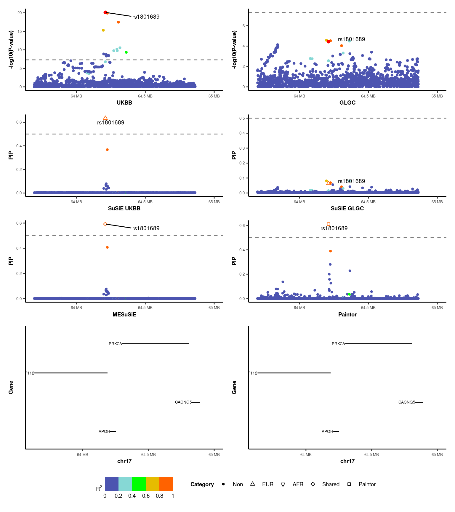
3c. TM6SF2 Example
#######################################################################
#
#           TM6SF2 gene and LDL association with ancestry-specific effect
#
#
##########################################################################

region = 275
trait_name = "LDL"
ref_panel = "UKB1"
p_threshold_index = 1
res_z_dir<-paste0("/net/fantasia/home/borang/Susie_Mult/Revision_Round_1/01_02_Real_Data/",trait_name,"/",trait_name,"_REF_",ref_panel,"_P",p_threshold_index,"/")
out_dir<-paste0(res_z_dir,"data/")
out_res_dir<-paste0(res_z_dir,"res/")

##Date Reprocess
WB_COV<-as.matrix(fread(paste0(out_dir,"Region_",region,".LD1")))
BB_COV<-as.matrix(fread(paste0(out_dir,"Region_",region,".LD2")))
load(paste0(out_res_dir,"MESuSiE_region_",region,".RData"))

candidate_region<-res_all%>%filter(Region==region)
# rs58542926 is the missense of TM6SF2 gene gene, highlighted in the paper
lead_SNP = "rs58542926"
lead_SNP_index<-which(candidate_region$SNP==lead_SNP)
candidate_region<-candidate_region%>%mutate(r2_EUR  = unname(unlist((WB_COV[,lead_SNP_index])^2)) ,r2_AFR = unname(unlist((BB_COV[,lead_SNP_index])^2)),POS = as.numeric(POS))
####Category Setting
candidate_region<-candidate_region%>%mutate(SuSiE_cat = case_when(SuSiE_WB>0.5&SuSiE_BB>0.5 ~ 3,
                                                                  SuSiE_WB>0.5&SuSiE_BB<0.5 ~ 1,
                                                                  SuSiE_WB<0.5&SuSiE_BB>0.5 ~ 2,
                                                                  TRUE ~ 0),
                                            Paintor_cat = case_when(Paintor_PIP>0.5~4,
                                                                    TRUE~0),
                                            MESuSiE_cat = case_when(MESuSiE_PIP_WB>0.5~1,
                                                                    MESuSiE_PIP_BB>0.5~2,
                                                                    MESuSiE_PIP_Shared>0.5~3,
                                                                    TRUE~0))
###GWAS PLOT
EUR_GWAS_plot_data<-candidate_region%>%mutate(r2 = r2_EUR,PIP = -log10(2*pnorm(-abs(zscore_WB))),Lead_SNP = ifelse(SNP==lead_SNP,1,0),POS= as.numeric(POS))%>%select(SNP,POS, r2,PIP,Lead_SNP)
AFR_GWAS_plot_data<-candidate_region%>%mutate(r2 = r2_AFR,PIP = -log10(2*pnorm(-abs(zscore_BB))),Lead_SNP = ifelse(SNP==lead_SNP,1,0),POS= as.numeric(POS))%>%select(SNP,POS, r2,PIP,Lead_SNP)
p_EUR<-gwas_plot_fun (EUR_GWAS_plot_data, "UKBB", "-log10(P-value)", -log10(5e-8))
p_AFR<-gwas_plot_fun (AFR_GWAS_plot_data, "GLGC", "-log10(P-value)", -log10(5e-8))

###Finemap Plot
EUR_SuSiE_plot_data<-candidate_region%>%mutate(r2 = r2_EUR,PIP = SuSiE_WB,Lead_SNP = ifelse(SNP==lead_SNP,1,0),POS= as.numeric(POS),cat = factor(SuSiE_cat,levels = c("0", "1", "2", "3", "4"), labels = c("Non", "EUR", "AFR", "Shared", "Paintor")))%>%select(SNP,POS, r2,PIP,Lead_SNP,cat)
AFR_SuSiE_plot_data<-candidate_region%>%mutate(r2 = r2_AFR,PIP = SuSiE_BB,Lead_SNP = ifelse(SNP==lead_SNP,1,0),POS= as.numeric(POS),cat = factor(SuSiE_cat,levels = c("0", "1", "2", "3", "4"), labels = c("Non", "EUR", "AFR", "Shared", "Paintor")))%>%select(SNP,POS, r2,PIP,Lead_SNP,cat)
MESuSiE_plot_data<-candidate_region%>%mutate(r2 = r2_EUR,PIP = MESuSiE_PIP_Either,Lead_SNP = ifelse(SNP==lead_SNP,1,0),POS= as.numeric(POS),cat = factor(MESuSiE_cat,levels = c("0", "1", "2", "3", "4"), labels = c("Non", "EUR", "AFR", "Shared", "Paintor")))%>%select(SNP,POS, r2,PIP,Lead_SNP,cat)
Paintor_plot_data<-candidate_region%>%mutate(r2 = r2_EUR,PIP = Paintor_PIP,Lead_SNP = ifelse(SNP==lead_SNP,1,0),POS= as.numeric(POS),cat = factor(Paintor_cat,levels = c("0", "1", "2", "3", "4"), labels = c("Non", "EUR", "AFR", "Shared", "Paintor")))%>%select(SNP,POS, r2,PIP,Lead_SNP,cat)

p_EUR_SuSiE<-finemap_plot_fun(EUR_SuSiE_plot_data, "SuSiE UKBB", "PIP", 0.5)
p_AFR_SuSiE<-finemap_plot_fun(AFR_SuSiE_plot_data, "SuSiE GLGC", "PIP", 0.5)
p_MESuSiE<-finemap_plot_fun(MESuSiE_plot_data, "MESuSiE", "PIP", 0.5)
p_Paintor<-finemap_plot_fun(Paintor_plot_data, "Paintor", "PIP", 0.5)

# Gene Plot
plot.range <- c(min(candidate_region$POS), max(candidate_region$POS))
Gene_List_sub_coding<-Gene_List%>%filter(Chrom==paste0("chr",unique(candidate_region$CHR)))%>%filter(Start<max(candidate_region$POS),End>min(candidate_region$POS))%>%filter(Coding=="proteincoding")%>%filter(!is.na(cdsLength))%>%filter(GeneLength>15000|Gene=="TM6SF2")
p2<-gene_range_plot_fun(Gene_List_sub_coding,plot.range)

##Combine Plot together
combined_plot<-(p_EUR/p_EUR_SuSiE/p_MESuSiE/p2+plot_layout(heights = c(1,1,1,1.5))|p_AFR/p_AFR_SuSiE/p_Paintor/p2+plot_layout(heights = c(1,1,1,1.5)))+plot_layout(guides = 'collect')&theme(legend.position = "bottom")
combined_plot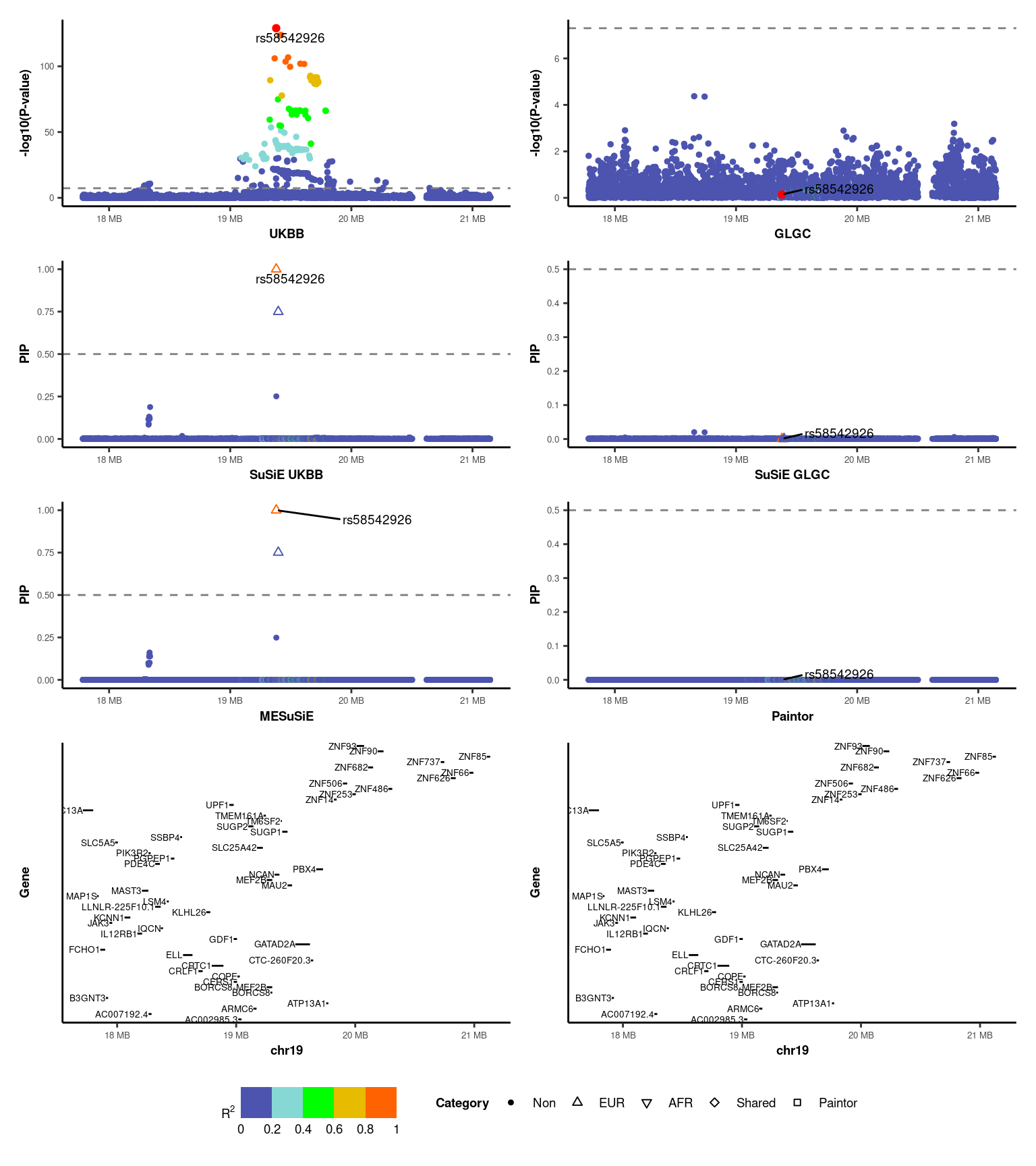
sessionInfo()R version 4.3.1 (2023-06-16)
Platform: x86_64-pc-linux-gnu (64-bit)
Running under: Ubuntu 20.04.6 LTS
Matrix products: default
BLAS: /usr/lib/x86_64-linux-gnu/openblas-pthread/libblas.so.3
LAPACK: /usr/lib/x86_64-linux-gnu/openblas-pthread/liblapack.so.3; LAPACK version 3.9.0
locale:
[1] LC_CTYPE=en_US.UTF-8 LC_NUMERIC=C
[3] LC_TIME=en_US.UTF-8 LC_COLLATE=en_US.UTF-8
[5] LC_MONETARY=en_US.UTF-8 LC_MESSAGES=en_US.UTF-8
[7] LC_PAPER=en_US.UTF-8 LC_NAME=C
[9] LC_ADDRESS=C LC_TELEPHONE=C
[11] LC_MEASUREMENT=en_US.UTF-8 LC_IDENTIFICATION=C
time zone: America/New_York
tzcode source: system (glibc)
attached base packages:
[1] grid stats graphics grDevices utils datasets methods
[8] base
other attached packages:
[1] stringr_1.5.0 ggrepel_0.9.1 susieR_0.11.84
[4] coin_1.4-2 survival_3.3-1 DescTools_0.99.45
[7] ggbreak_0.1.1 gridExtra_2.3 VennDiagram_1.7.3
[10] futile.logger_1.4.3 ggpmisc_0.4.7 ggpp_0.4.4
[13] patchwork_1.1.1 tidyr_1.3.0 dplyr_1.1.2
[16] data.table_1.14.8 ggpubr_0.6.0 ggplot2_3.4.2
[19] workflowr_1.7.0
loaded via a namespace (and not attached):
[1] formatR_1.14 gld_2.6.5 sandwich_3.0-2
[4] readxl_1.4.2 rlang_1.1.1 magrittr_2.0.3
[7] git2r_0.32.0 multcomp_1.4-25 matrixStats_1.0.0
[10] e1071_1.7-13 compiler_4.3.1 mgcv_1.8-40
[13] getPass_0.2-2 callr_3.7.3 vctrs_0.6.2
[16] quantreg_5.95 crayon_1.5.2 pkgconfig_2.0.3
[19] fastmap_1.1.1 backports_1.4.1 labeling_0.4.2
[22] utf8_1.2.3 promises_1.2.0.1 rmarkdown_2.22
[25] ps_1.7.2 MatrixModels_0.5-1 purrr_1.0.1
[28] xfun_0.39 modeltools_0.2-23 cachem_1.0.8
[31] aplot_0.1.10 jsonlite_1.8.3 highr_0.10
[34] later_1.3.1 reshape_0.8.9 irlba_2.3.5.1
[37] broom_1.0.5 parallel_4.3.1 R6_2.5.1
[40] bslib_0.5.0 stringi_1.7.12 car_3.1-2
[43] boot_1.3-28.1 jquerylib_0.1.4 cellranger_1.1.0
[46] Rcpp_1.0.11 knitr_1.39 zoo_1.8-12
[49] httpuv_1.6.11 Matrix_1.5-4.1 splines_4.3.1
[52] tidyselect_1.2.0 rstudioapi_0.14 abind_1.4-5
[55] yaml_2.3.7 codetools_0.2-19 processx_3.8.0
[58] plyr_1.8.8 lattice_0.20-45 tibble_3.2.1
[61] withr_2.5.1 evaluate_0.18 gridGraphics_0.5-1
[64] lambda.r_1.2.4 proxy_0.4-27 pillar_1.9.0
[67] carData_3.0-5 whisker_0.4.1 stats4_4.3.1
[70] ggfun_0.0.9 generics_0.1.3 rprojroot_2.0.3
[73] munsell_0.5.0 scales_1.2.1 rootSolve_1.8.2.3
[76] class_7.3-20 glue_1.6.2 lmom_2.8
[79] tools_4.3.1 SparseM_1.81 ggsignif_0.6.4
[82] Exact_3.1 fs_1.6.2 mvtnorm_1.1-3
[85] libcoin_1.0-9 colorspace_2.1-0 nlme_3.1-157
[88] cli_3.6.1 futile.options_1.0.1 fansi_1.0.5
[91] expm_0.999-7 mixsqp_0.3-48 gtable_0.3.1
[94] rstatix_0.7.2 yulab.utils_0.0.4 sass_0.4.6
[97] digest_0.6.30 TH.data_1.1-2 ggplotify_0.1.0
[100] farver_2.1.1 htmltools_0.5.5 lifecycle_1.0.3
[103] httr_1.4.6 MASS_7.3-57