Run MESuSiE
borangao
2023-10-09
Last updated: 2023-10-09
Checks: 6 1
Knit directory: meSuSie_Analysis/
This reproducible R Markdown analysis was created with workflowr (version 1.7.0). The Checks tab describes the reproducibility checks that were applied when the results were created. The Past versions tab lists the development history.
Great! Since the R Markdown file has been committed to the Git repository, you know the exact version of the code that produced these results.
Great job! The global environment was empty. Objects defined in the global environment can affect the analysis in your R Markdown file in unknown ways. For reproduciblity it’s best to always run the code in an empty environment.
The command set.seed(20220530) was run prior to running
the code in the R Markdown file. Setting a seed ensures that any results
that rely on randomness, e.g. subsampling or permutations, are
reproducible.
Great job! Recording the operating system, R version, and package versions is critical for reproducibility.
Nice! There were no cached chunks for this analysis, so you can be confident that you successfully produced the results during this run.
Using absolute paths to the files within your workflowr project makes it difficult for you and others to run your code on a different machine. Change the absolute path(s) below to the suggested relative path(s) to make your code more reproducible.
| absolute | relative |
|---|---|
| /net/fantasia/home/borang/Susie_Mult/meSuSie_Analysis/data/MESuSiE_Example.RData | data/MESuSiE_Example.RData |
Great! You are using Git for version control. Tracking code development and connecting the code version to the results is critical for reproducibility.
The results in this page were generated with repository version 62ce4b3. See the Past versions tab to see a history of the changes made to the R Markdown and HTML files.
Note that you need to be careful to ensure that all relevant files for
the analysis have been committed to Git prior to generating the results
(you can use wflow_publish or
wflow_git_commit). workflowr only checks the R Markdown
file, but you know if there are other scripts or data files that it
depends on. Below is the status of the Git repository when the results
were generated:
Untracked files:
    Untracked:  data/GLGC_chr_22.txt
    Untracked:  data/MESuSiE_Example.RData
    Untracked:  data/UKBB_chr_22.txt

Unstaged changes:
    Modified:   analysis/_site.yml
    Modified:   analysis/about.Rmd
    Deleted:    analysis/illustration.Rmd
    Deleted:    analysis/toy_example.Rmd
Note that any generated files, e.g. HTML, png, CSS, etc., are not included in this status report because it is ok for generated content to have uncommitted changes.
These are the previous versions of the repository in which changes were
made to the R Markdown (analysis/Run_MESuSiE.Rmd) and HTML
(docs/Run_MESuSiE.html) files. If you’ve configured a
remote Git repository (see ?wflow_git_remote), click on the
hyperlinks in the table below to view the files as they were in that
past version.
| File | Version | Author | Date | Message |
|---|---|---|---|---|
| Rmd | 62ce4b3 | borangao | 2023-10-09 | Update my analysis |
MESuSiE Example
1. Data Formatting for MESuSiE:
Use the example from Data preparation. We provide
organize data and organize_ld function to do
the sanity check and organize the summary statistics and LD into the
MESuSiE input format
library(dplyr)
library(MESuSiE)
load("/net/fantasia/home/borang/Susie_Mult/meSuSie_Analysis/data/MESuSiE_Example.RData")
summ_stat_list<-organize_gwas(UKBB_example%>%rename(SNP = CHR_POS),GLGC_example%>%rename(SNP = CHR_POS),c("EUR","AFR"))
colnames(WB_cov)<-UKBB_example$CHR_POS
colnames(BB_cov)<-GLGC_example$CHR_POS
LD_list<-organize_ld(WB_cov,BB_cov,summ_stat_list)
2. Run MESuSiE:
MESuSiE_res<-meSuSie_core(LD_list,summ_stat_list,L=10)*************************************************************
Multiple Ancestry Sum of Single Effect Model (MESuSiE)
Visit http://www.xzlab.org/software.html For Update
(C) 2022 Boran Gao, Xiang Zhou
GNU General Public License
*************************************************************
# Start data processing for sufficient statistics
# Create MESuSiE object
# Start data analysis
# Data analysis is done, and now generates result
Potential causal SNPs with PIP > 0.5: 22_21958872
Credible sets for effects:
$cs
$cs$L1
[1] 7 8 26 38 40 41 57 61 62 69 71 79 82
$cs_category
L1
"EUR_AFR"
$purity
min.abs.corr mean.abs.corr median.abs.corr
L1 0.9978499 0.9991224 0.9992341
$cs_index
[1] 1
$coverage
[1] 0.9551583
$requested_coverage
[1] 0.95
Use MESuSiE_Plot() for visualization
# Total time used for the analysis: 0.07 minsMESuSiE Result Interpretation:
The MESuSiE results can be interpreted in terms of the 95% credible set and SNP-level Posterior Inclusion Probabilities (PIPs).
- 95% credible set MESuSiE’s 95% credible set comprises SNPs with a non-zero effect in at least one ancestry. These SNPs are further categorized as either “shared” or “ancestry-specific” based on their contribution to the credible set.
For instance, in the provided example, the credible set contains 13
SNPs labeled as EUR_AFR, indicating these SNPs are shared
across multiple ancestries.
PIPs We used a PIP cutoff of 0.5 to declare signal.
- PIP for SNP have non-zero effect in at least one ancestry
MESuSiE_res$pip[MESuSiE_res$cs$cs$L1][1] 0.02617149 0.02411160 0.04600253 0.03558618 0.02805318 0.03538103 [7] 0.02041509 0.05667729 0.05446116 0.04994392 0.52385726 0.02241395 [13] 0.03208367In the example provided, one SNP exhibits a PIP greater than 0.5. However, this does not inform us whether the SNP is shared or ancestry-specific. To make that inference, we need to further analyze the PIP values for shared or ancestry-specific effects, which is the unique feature provided by MESuSiE.
- PIP for shared or ancestry-specific effect
MESuSiE_res$pip_config[MESuSiE_res$cs$cs$L1,]EUR AFR EUR_AFR [1,] 0.0003748811 0.0002535134 0.02617115 [2,] 0.0003748810 0.0002532205 0.02411128 [3,] 0.0003748798 0.0002476710 0.04600234 [4,] 0.0003748806 0.0002482805 0.03558589 [5,] 0.0003748802 0.0002483030 0.02805295 [6,] 0.0003748805 0.0002483253 0.03538074 [7,] 0.0003748796 0.0002484404 0.02041492 [8,] 0.0003748794 0.0002484522 0.05667714 [9,] 0.0003748793 0.0002485671 0.05446102 [10,] 0.0003748793 0.0002480695 0.04994379 [11,] 0.0003748793 0.0002610915 0.52385712 [12,] 0.0003748795 0.0002468203 0.02241380 [13,] 0.0003748793 0.0002458986 0.03208353From the results, SNP with a PIP greater than 0.5 represents a shared causal signal.
3.Configuring Tuning Parameters
When running meSuSie_core, various tuning parameters can
be adjusted to refine the results:
- Number of Effects (
L): Specify the number of effects to consider. - Prior Weights (
prior_weights): This represents the prior probability of a SNP being causal. By default, it is set to . Users can adjust this parameter to incorporate functional annotation into MESuSiE. - Ancestry Weight (
ancestry_weight): Configure the weighting for different ancestries. We set the ratio of ancestry-specific to shared as 3:1 to encourage the ancestry-specific causal SNP detection.- Pure shared signal: ancestry weight can be set to c(0,0,1)
- Encourage Ancestry-specific signal ancestry weight can be set to c(5,5,1)/sum(c(5,5,1))
- Estimate Residual Variance
(
estimate_residual_variance): This parameter can be set to either TRUE or FALSE. When set to TRUE, the residual variance is estimated, while when set to FALSE, it is fixed at one. For multi-ancestry GWAS fine-mapping, it’s typically advisable to fix the residual variance at one to enhance robustness, given that the heritability of the local region is often minimal. However, when using MESuSiE for multi-ancestry eQTL fine-mapping, it’s recommended to estimate the residual variance since the heritability of the gene expression is relatively significant. - Correlation Method and Threshold
(
cor_method & cor_threshold):- cor_method: Choose the method to determine the 95%
credible set based on SNP correlations within the region. Commonly used
methods include determining the minimum, mean, or median of the absolute
correlation values. By default, this is set to
min_abs_corr, representing the minimum absolute correlation permissible within a credible set across ancestries. This is a prevalent threshold for genotype data in genetic studies. - cor_threshold: Define the cutoff for
min_abs_corr. By default, this is set to 0.5.
- cor_method: Choose the method to determine the 95%
credible set based on SNP correlations within the region. Commonly used
methods include determining the minimum, mean, or median of the absolute
correlation values. By default, this is set to
Note: We’ve made available function
meSuSie_get_csallowing users to tweak the results based on varyingcor_methodandcor_threshold. The best part? You can adjust without having to rerun the entire analysis.
4. MESuSiE Visulization:
MESuSiE_Plot(MESuSiE_res,LD_list,summ_stat_list)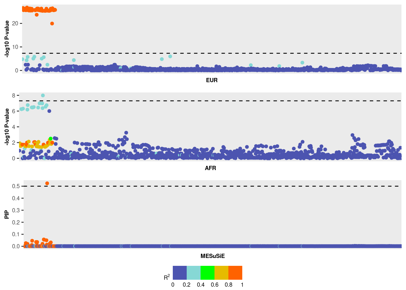
sessionInfo()R version 4.3.1 (2023-06-16)
Platform: x86_64-pc-linux-gnu (64-bit)
Running under: Ubuntu 20.04.6 LTS
Matrix products: default
BLAS: /usr/lib/x86_64-linux-gnu/openblas-pthread/libblas.so.3
LAPACK: /usr/lib/x86_64-linux-gnu/openblas-pthread/liblapack.so.3; LAPACK version 3.9.0
locale:
[1] LC_CTYPE=en_US.UTF-8 LC_NUMERIC=C
[3] LC_TIME=en_US.UTF-8 LC_COLLATE=en_US.UTF-8
[5] LC_MONETARY=en_US.UTF-8 LC_MESSAGES=en_US.UTF-8
[7] LC_PAPER=en_US.UTF-8 LC_NAME=C
[9] LC_ADDRESS=C LC_TELEPHONE=C
[11] LC_MEASUREMENT=en_US.UTF-8 LC_IDENTIFICATION=C
time zone: America/New_York
tzcode source: system (glibc)
attached base packages:
[1] stats graphics grDevices utils datasets methods base
other attached packages:
[1] MESuSiE_1.0 dplyr_1.1.2 workflowr_1.7.0
loaded via a namespace (and not attached):
[1] gtable_0.3.1 xfun_0.39 bslib_0.5.0
[4] ggplot2_3.4.2 processx_3.8.0 ggrepel_0.9.1
[7] lattice_0.20-45 callr_3.7.3 vctrs_0.6.2
[10] tools_4.3.1 ps_1.7.2 generics_0.1.3
[13] tibble_3.2.1 fansi_1.0.5 highr_0.10
[16] pkgconfig_2.0.3 Matrix_1.5-4.1 data.table_1.14.8
[19] lifecycle_1.0.3 compiler_4.3.1 farver_2.1.1
[22] stringr_1.5.0 git2r_0.32.0 progress_1.2.2
[25] munsell_0.5.0 getPass_0.2-2 httpuv_1.6.11
[28] htmltools_0.5.5 sass_0.4.6 yaml_2.3.7
[31] later_1.3.1 pillar_1.9.0 nloptr_2.0.3
[34] crayon_1.5.2 jquerylib_0.1.4 whisker_0.4.1
[37] tidyr_1.3.0 ellipsis_0.3.2 cachem_1.0.8
[40] tidyselect_1.2.0 digest_0.6.30 stringi_1.7.12
[43] purrr_1.0.1 labeling_0.4.2 RcppArmadillo_0.11.1.1.0
[46] cowplot_1.1.1 rprojroot_2.0.3 fastmap_1.1.1
[49] grid_4.3.1 colorspace_2.1-0 cli_3.6.1
[52] magrittr_2.0.3 utf8_1.2.3 withr_2.5.1
[55] prettyunits_1.2.0 scales_1.2.1 promises_1.2.0.1
[58] rmarkdown_2.22 httr_1.4.6 hms_1.1.2
[61] evaluate_0.18 knitr_1.39 irlba_2.3.5.1
[64] rlang_1.1.1 Rcpp_1.0.11 mixsqp_0.3-48
[67] glue_1.6.2 rstudioapi_0.14 jsonlite_1.8.3
[70] R6_2.5.1 fs_1.6.2