Merging and interpolation of observations
Jens Daniel Müller
25 September, 2020
Last updated: 2020-09-25
Checks: 7 0
Knit directory: BloomSail/
This reproducible R Markdown analysis was created with workflowr (version 1.6.2). The Checks tab describes the reproducibility checks that were applied when the results were created. The Past versions tab lists the development history.
Great! Since the R Markdown file has been committed to the Git repository, you know the exact version of the code that produced these results.
Great job! The global environment was empty. Objects defined in the global environment can affect the analysis in your R Markdown file in unknown ways. For reproduciblity it’s best to always run the code in an empty environment.
The command set.seed(20191021) was run prior to running the code in the R Markdown file. Setting a seed ensures that any results that rely on randomness, e.g. subsampling or permutations, are reproducible.
Great job! Recording the operating system, R version, and package versions is critical for reproducibility.
Nice! There were no cached chunks for this analysis, so you can be confident that you successfully produced the results during this run.
Great job! Using relative paths to the files within your workflowr project makes it easier to run your code on other machines.
Great! You are using Git for version control. Tracking code development and connecting the code version to the results is critical for reproducibility.
The results in this page were generated with repository version abc5bac. See the Past versions tab to see a history of the changes made to the R Markdown and HTML files.
Note that you need to be careful to ensure that all relevant files for the analysis have been committed to Git prior to generating the results (you can use wflow_publish or wflow_git_commit). workflowr only checks the R Markdown file, but you know if there are other scripts or data files that it depends on. Below is the status of the Git repository when the results were generated:
Ignored files:
    Ignored:    .Rhistory
    Ignored:    .Rproj.user/
    Ignored:    data/Finnmaid_2018/
    Ignored:    data/GETM/
    Ignored:    data/Maps/
    Ignored:    data/Ostergarnsholm/
    Ignored:    data/TinaV/
    Ignored:    data/_merged_data_files/
    Ignored:    data/_summarized_data_files/
    Ignored:    data/backup/
    Ignored:    output/Plots/Figures_publication/.tmp.drivedownload/

Untracked files:
    Untracked:  code/Vertical entrainment flux I.pdf
    Untracked:  code/Vertical entrainment flux II.pdf
    Untracked:  code/Vertical entrainment flux III.pdf
    Untracked:  output/Plots/Figures_publication/Appendix/Phytoplankton_mean_total_biomass.png
    Untracked:  output/Plots/Figures_publication/Appendix/TPD_CPD_cumulative.png
    Untracked:  output/Plots/Figures_publication/Appendix/pCO2_RT_corrected_profile_example.png
    Untracked:  output/Plots/Figures_publication/Appendix/pCO2_RT_corrected_profile_mean_abs_offset.png
    Untracked:  output/Plots/Figures_publication/Appendix/tau_fit_example.png
    Untracked:  output/Plots/Figures_publication/Appendix/tb_profiles.png
    Untracked:  output/Plots/Figures_publication/Article/Hov_abs_profiles_cum.png
    Untracked:  output/Plots/Figures_publication/Article/atm_water_timeseries.png
    Untracked:  output/Plots/Figures_publication/Article/data_coverage.png
    Untracked:  output/Plots/Figures_publication/Article/profiles_all.png
    Untracked:  output/Plots/Figures_publication/Article/reconstruction_NCP_timeseries.png
    Untracked:  output/Plots/Figures_publication/Article/reconstruction_iCT_timeseries.png
    Untracked:  output/Plots/Figures_publication/Article/station_map.png

Unstaged changes:
    Modified:   analysis/read-in.Rmd
    Modified:   output/Plots/CT_dynamics/tm_profiles_ID_pCO2_tem_sal_CT.pdf
    Modified:   output/Plots/Figures_publication/Appendix/Phytoplankton_mean_total_biomass.pdf
    Modified:   output/Plots/Figures_publication/Appendix/TPD_CPD_cumulative.pdf
    Modified:   output/Plots/Figures_publication/Appendix/pCO2_RT_corrected_profile_example.pdf
    Modified:   output/Plots/Figures_publication/Appendix/pCO2_RT_corrected_profile_mean_abs_offset.pdf
    Modified:   output/Plots/Figures_publication/Appendix/tau_fit_example.pdf
    Modified:   output/Plots/Figures_publication/Appendix/tb_profiles.pdf
    Modified:   output/Plots/Figures_publication/Article/Hov_abs_profiles_cum.pdf
    Modified:   output/Plots/Figures_publication/Article/atm_water_timeseries.pdf
    Modified:   output/Plots/Figures_publication/Article/data_coverage.pdf
    Modified:   output/Plots/Figures_publication/Article/profiles_all.pdf
    Modified:   output/Plots/Figures_publication/Article/reconstruction_NCP_timeseries.pdf
    Modified:   output/Plots/Figures_publication/Article/reconstruction_iCT_timeseries.pdf
    Modified:   output/Plots/Figures_publication/Article/station_map.pdf
    Modified:   output/Plots/merging_interpolation/Zero_time_synchronization.pdf
Note that any generated files, e.g. HTML, png, CSS, etc., are not included in this status report because it is ok for generated content to have uncommitted changes.
These are the previous versions of the repository in which changes were made to the R Markdown (analysis/merging_interpolation.Rmd) and HTML (docs/merging_interpolation.html) files. If you’ve configured a remote Git repository (see ?wflow_git_remote), click on the hyperlinks in the table below to view the files as they were in that past version.
| File | Version | Author | Date | Message |
|---|---|---|---|---|
| Rmd | abc5bac | jens-daniel-mueller | 2020-09-25 | comparison of pCO2 data included |
| html | 904f0f7 | jens-daniel-mueller | 2020-09-23 | Build site. |
| Rmd | 7f497e4 | jens-daniel-mueller | 2020-09-23 | updated tau lm fit procedure |
| html | 8951791 | jens-daniel-mueller | 2020-09-23 | Build site. |
| Rmd | 9e87621 | jens-daniel-mueller | 2020-09-23 | included postprocessed cleaned data |
| html | ddd2d3e | jens-daniel-mueller | 2020-09-23 | Build site. |
| Rmd | 3ad71b0 | jens-daniel-mueller | 2020-09-23 | included postprocessed cleaned data |
| html | aea9be2 | jens-daniel-mueller | 2020-09-23 | Build site. |
| Rmd | ed17078 | jens-daniel-mueller | 2020-09-23 | included postprocessed cleaned data |
| html | 66bf52a | jens-daniel-mueller | 2020-09-23 | Build site. |
| Rmd | 0c8eed6 | jens-daniel-mueller | 2020-09-23 | included postprocessed cleaned data |
| html | c919fb7 | jens-daniel-mueller | 2020-06-29 | Build site. |
| Rmd | 1461cb6 | jens-daniel-mueller | 2020-06-29 | Fig update for talk |
| html | 603af23 | jens-daniel-mueller | 2020-05-25 | Build site. |
| html | 3414c23 | jens-daniel-mueller | 2020-05-25 | Build site. |
| html | 772e588 | jens-daniel-mueller | 2020-05-04 | Build site. |
| Rmd | 2ab39d7 | jens-daniel-mueller | 2020-05-04 | All profiles and timeseries in one plot pdf |
| html | 1ae50d3 | jens-daniel-mueller | 2020-05-04 | Build site. |
| Rmd | e78c435 | jens-daniel-mueller | 2020-05-04 | finalized time sync check |
| html | f95bf94 | jens-daniel-mueller | 2020-05-04 | Build site. |
| Rmd | 56f6c8a | jens-daniel-mueller | 2020-05-04 | corrected dep_maxgap removel criterion |
| html | c23350e | jens-daniel-mueller | 2020-05-04 | Build site. |
| Rmd | 3067532 | jens-daniel-mueller | 2020-05-04 | revise time sync |
| html | 3832733 | jens-daniel-mueller | 2020-04-30 | Build site. |
| Rmd | 4f4ab08 | jens-daniel-mueller | 2020-04-30 | harmonized code until RT determination |
| html | 6465570 | jens-daniel-mueller | 2020-04-29 | Build site. |
| Rmd | 0bbf0e6 | jens-daniel-mueller | 2020-04-29 | revised nomenclature |
| html | ebd1948 | jens-daniel-mueller | 2020-04-29 | Build site. |
| Rmd | 52090bf | jens-daniel-mueller | 2020-04-29 | correct interpolation, new d pco2 plot range |
| html | d9248a6 | jens-daniel-mueller | 2020-04-29 | Build site. |
| Rmd | 70bd3f0 | jens-daniel-mueller | 2020-04-29 | correct interpolation, new d pco2 plot |
| html | b5722a7 | jens-daniel-mueller | 2020-04-28 | Build site. |
| html | 472c2b4 | jens-daniel-mueller | 2020-04-21 | Build site. |
| html | f8fcf50 | jens-daniel-mueller | 2020-04-19 | created pub figures for time series |
| html | a6c4c22 | jens-daniel-mueller | 2020-03-30 | Build site. |
| html | 80c78b3 | jens-daniel-mueller | 2020-03-30 | Build site. |
| html | 5f8ca30 | jens-daniel-mueller | 2020-03-20 | Build site. |
| html | 2a20453 | jens-daniel-mueller | 2020-03-20 | Build site. |
| html | 473ab25 | jens-daniel-mueller | 2020-03-19 | Build site. |
| html | 81f022e | jens-daniel-mueller | 2020-03-18 | Build site. |
| html | 1e39d85 | jens-daniel-mueller | 2020-03-18 | Build site. |
| html | 2105236 | jens-daniel-mueller | 2020-03-18 | Build site. |
| html | 05b9bdc | jens-daniel-mueller | 2020-03-17 | Build site. |
| html | 0202742 | jens-daniel-mueller | 2020-03-16 | Build site. |
| html | 8e83afd | jens-daniel-mueller | 2020-03-12 | Build site. |
| html | a3ddea4 | jens-daniel-mueller | 2020-03-12 | Build site. |
| html | 52621ea | jens-daniel-mueller | 2020-03-12 | Build site. |
| html | e43a6f2 | jens-daniel-mueller | 2019-12-19 | Build site. |
| html | 3042ff3 | jens-daniel-mueller | 2019-12-19 | Build site. |
| Rmd | 282c3ac | jens-daniel-mueller | 2019-12-19 | whole data set RT corrected |
| html | 78710ee | jens-daniel-mueller | 2019-12-09 | Build site. |
| Rmd | c6cfca5 | jens-daniel-mueller | 2019-12-09 | RT correction incl OGB data |
| html | c6cfca5 | jens-daniel-mueller | 2019-12-09 | RT correction incl OGB data |
| html | bc6f19b | jens-daniel-mueller | 2019-11-22 | Build site. |
| Rmd | 03b1b97 | jens-daniel-mueller | 2019-11-22 | updated RT determination |
| html | 874dac5 | jens-daniel-mueller | 2019-11-22 | Build site. |
| Rmd | f875795 | jens-daniel-mueller | 2019-11-22 | now clean |
| html | d921065 | jens-daniel-mueller | 2019-11-14 | Build site. |
| Rmd | 252f84d | jens-daniel-mueller | 2019-11-14 | included EDA in data base |
| html | d61a468 | jens-daniel-mueller | 2019-11-14 | Build site. |
| html | f3277a5 | jens-daniel-mueller | 2019-11-08 | Build site. |
| html | 4256bcf | jens-daniel-mueller | 2019-11-08 | Build site. |
| html | 72687ee | jens-daniel-mueller | 2019-11-08 | Build site. |
| html | 74212a6 | jens-daniel-mueller | 2019-11-08 | Build site. |
| Rmd | 6cb1935 | jens-daniel-mueller | 2019-11-08 | response_time updated |
| html | 33e3659 | jens-daniel-mueller | 2019-10-22 | Build site. |
| Rmd | efcafd1 | jens-daniel-mueller | 2019-10-22 | Added data base, merging, and RT determination |
| html | 1595fe9 | jens-daniel-mueller | 2019-10-21 | Build site. |
| Rmd | 4131b9c | jens-daniel-mueller | 2019-10-21 | finisehd read CTD and HydroC, created merging Rmd |
library(tidyverse)
library(lubridate)
library(zoo)
1 CTD (ts) + HydroC CO2 data (th)
1.1 Merging summarized data sets
# Load Sensor and HydroC data ---------------------------------------------
ts <- read_csv(here::here("Data/_summarized_data_files",
                          "ts.csv"),
               col_types = list("pCO2_analog" = col_double()))

th <- read_csv(here::here("Data/_summarized_data_files",
                          "th.csv"))

# Time offset correction ----------------------------------------------

# Time offset was determined by comparing zeroing reads from Sensor and th
# in the plots produced in the section Time stamp synchronicity below
# before applying this correction

ts <- ts %>%
  mutate(day = yday(date_time),
         date_time = if_else(day >= 206 & day <= 220,
                             date_time - 80, date_time - 10)) %>%
  select(-day)

# Merge Sensor and HydroC data --------------------------------------------

ts_th <- full_join(ts, th) %>%
  arrange(date_time)

# ts_th_full <- full_join(ts, th_full) %>%
#   arrange(date_time)

rm(th, ts)
1.2 Interpolation to common time stamp
CTD and auxillary recordings (15 sec measurment interval) are interpolated to HydroC time stamps (first 10 sec, than 1 sec measurement interval) when gaps between observations are not larger than 20. Thereafter, HydroC readings not falling in regular transects/profilings are removed, by removing rows with NA depth values. Furthermore, CTD readings without corresponding HydroC reading are removed, except during periods when HydroC was not operating.
# Interpolate Sensor data to HydroC time stamp

ts_th <- ts_th %>%
  mutate(dep_maxgap = na.approx(dep, na.rm = FALSE, maxgap = 20),
         dep = approxfun(date_time, dep)(date_time),
         sal = approxfun(date_time, sal)(date_time),
         tem = approxfun(date_time, tem)(date_time),
         pCO2_analog = approxfun(date_time, pCO2_analog)(date_time)) %>%
  filter(!is.na(dep_maxgap)) %>% #remove HC readings not falling in regular transects/profiling
  select(- dep_maxgap) %>%
  fill(ID, type, station) %>%
  filter(!is.na(deployment), !is.na(pCO2_analog)) # removes CTD readings without corresponding HydroC reading

  # filter(!is.na(deployment) | is.na(pCO2_analog)) # removes CTD readings without corresponding HydroC reading, except during periods when HydroC was not operating


# Time stamp synchronicity

ts_th_Zero <- ts_th %>%
  filter(Zero == 1 | Flush == 1 & duration < 120)

pdf(file=here::here("output/Plots/merging_interpolation",
                    "Zero_time_synchronization.pdf"),
    onefile = TRUE, width = 5, height = 5)

for (i_deployment in unique(ts_th$deployment)) {

  #i_deployment <- unique(ts_th_Zero$deployment)[1]

  ts_th_Zero_deployment <- ts_th_Zero %>%
    filter(deployment == i_deployment)

  for (i_Zero_counter in unique(ts_th_Zero_deployment$Zero_counter)) {

    #i_Zero_counter <- unique(ts_th_Zero_deployment$Zero_counter)[1]

    print(

    ts_th_Zero_deployment %>%
      filter(Zero_counter == i_Zero_counter) %>%
      ggplot()+
      geom_point(aes(date_time, pCO2_corr, col="HydroC"))+
      geom_point(aes(date_time, pCO2_analog, col="analog"))+
      labs(title = paste("Depl: ",i_deployment,
                         " | Zero_counter: ", i_Zero_counter))

    )

  }
}

dev.off()

rm(ts_th_Zero, ts_th_Zero_deployment, i_deployment, i_Zero_counter)
1.3 Write merged file
ts_th %>%
  write_csv(here::here("Data/_merged_data_files/merging_interpolation", "ts_th.csv"))

rm(ts_th)
1.4 Time series pCO2
1.4.1 Read cleaned processed data
HydroC pCO2 data were provided by KM Contros after applying a drift correction to the raw data, which was based on pre- and post-deployment calibration results.
# Read Contros corrected data file, based on cleaned recordings

th_new_withAW <-
  read_csv2(here::here("Data/TinaV/Sensor/HydroC-pCO2/corrected_Contros",
                       "parameter&pCO2s(method 43)_new_withAW.txt"),
            col_names = c("date_time", "Zero", "Flush", "p_NDIR",
                          "p_in", "T_control", "T_gas", "%rH_gas",
                          "Signal_raw", "Signal_ref", "T_sensor",
                          "pCO2_corr", "Runtime", "nr.ave")) %>%
  mutate(date_time = dmy_hms(date_time),
         Flush = as.factor(as.character(Flush)),
         Zero = as.factor(as.character(Zero)))

# Read Contros corrected data file, based on cleaned recordings without water vapor correction

th_new_withoutAW <-
  read_csv2(here::here("Data/TinaV/Sensor/HydroC-pCO2/corrected_Contros",
                       "parameter&pCO2s(method 43)_new_withoutAW.txt"),
            col_names = c("date_time", "Zero", "Flush", "p_NDIR",
                          "p_in", "T_control", "T_gas", "%rH_gas",
                          "Signal_raw", "Signal_ref", "T_sensor",
                          "pCO2_corr", "Runtime", "nr.ave")) %>%
  mutate(date_time = dmy_hms(date_time),
         Flush = as.factor(as.character(Flush)),
         Zero = as.factor(as.character(Zero)))

th_all_data <- read_csv(here::here("Data/_summarized_data_files",
                          "th_all_data.csv"))


ts_th <- read_csv(here::here("data/_merged_data_files/merging_interpolation",
                          "ts_th.csv"),
               col_types = cols(ID = col_character(),
                                pCO2_analog = col_double(),
                                pCO2_corr = col_double(),
                                Zero = col_factor(),
                                Flush = col_factor(),
                                Zero_counter = col_integer(),
                                deployment = col_integer(),
                                duration = col_double(),
                                mixing = col_character()))
1.4.2 Comparison of preliminary pCO2 data
1.4.2.1 Analog vs internal
ggplot()+
  geom_path(data = th_all_data, aes(date_time, pCO2_corr, col = "pre cleaning"))+
  geom_path(data = ts_th, aes(date_time, pCO2_corr, col = "HydroC, drift corrected"))+
  geom_path(data = ts_th, aes(date_time, pCO2_analog, col = "analog CTD"))+
  scale_color_brewer(palette = "Set1", name = "pCO2 record")+
  coord_cartesian(ylim = c(0,600))+
  labs(y=expression(pCO[2]~(µatm)), x="")+
  facet_wrap(~deployment, scales = "free_x", ncol = 1)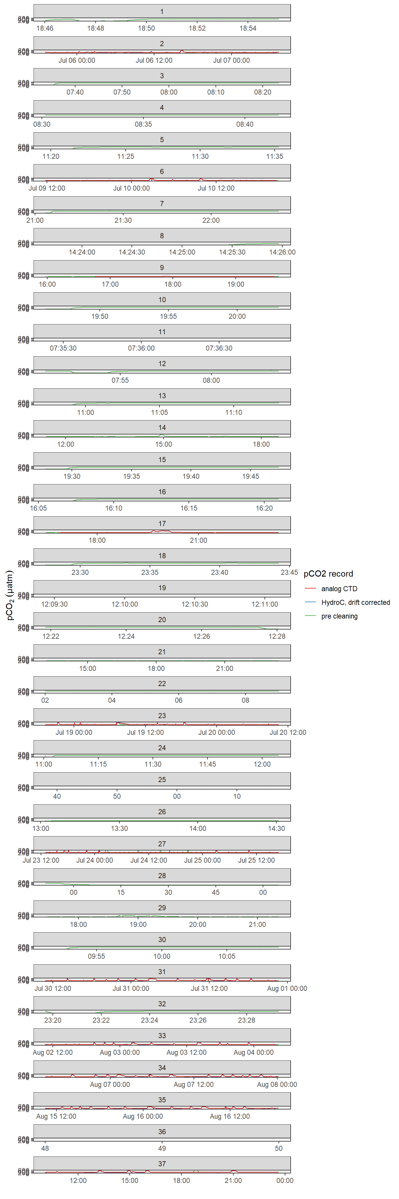
pCO2 record after interpolation to HydroC timestamp (analog output from HydroC and drift corrected data provided by Contos). ID refers to the starting date of each cruise. Please note that pCO2_analog measurement range is technically restricted to 100-500 µatm. Zeroing periods are included.
1.4.2.2 Raw vs clean
th_comparison <- full_join(
  ts_th %>% select(date_time, ID, pCO2_corr),
  th_new_withAW %>% select(date_time, pCO2_corr) %>% rename(pCO2_withAW = pCO2_corr)
)

th_comparison <- full_join(
  th_comparison,
  th_new_withoutAW %>% select(date_time, pCO2_corr) %>% rename(pCO2_withoutAW = pCO2_corr)
)


th_comparison %>%
  ggplot() +
  geom_path(aes(date_time, pCO2_corr, col = "HydroC, drift corrected"))+
  geom_path(aes(date_time, pCO2_withAW, col = "withAW"))+
  geom_path(aes(date_time, pCO2_withoutAW, col = "withoutAW"))+
  scale_color_brewer(palette = "Set1", name = "pCO2 record")+
  coord_cartesian(ylim = c(0,600))+
  labs(y=expression(pCO[2]~(µatm)), x="")+
  facet_wrap(~ID, scales = "free_x", ncol = 1)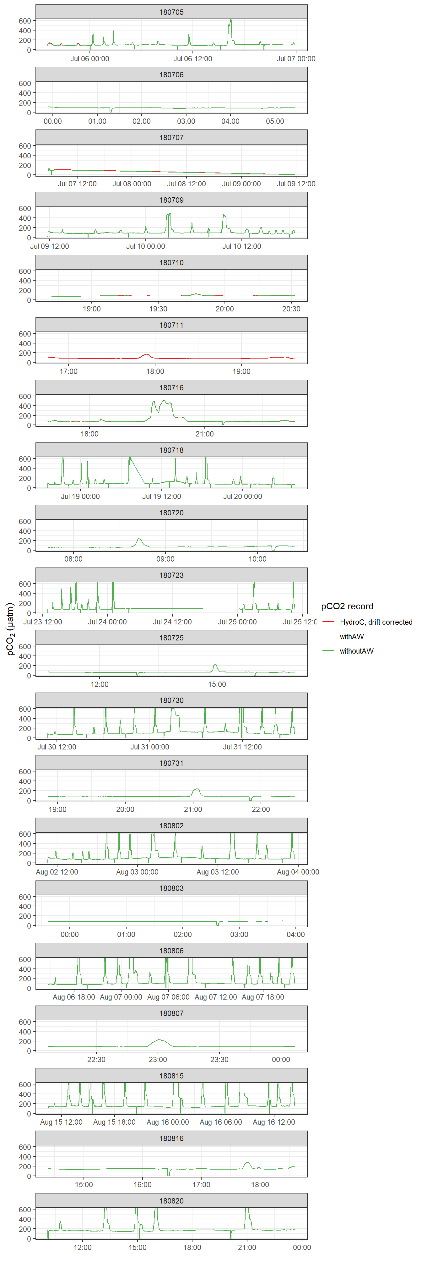
1.4.2.3 Water vapor correction
th_comparison %>%
  ggplot() +
  geom_path(aes(date_time, pCO2_corr-pCO2_withAW, col = "orig - with AW"))+
  scale_color_brewer(palette = "Set1", name = "pCO2 record")+
  labs(y=expression(pCO[2]~(µatm)), x="")+
  facet_wrap(~ID, scales = "free_x", ncol = 1)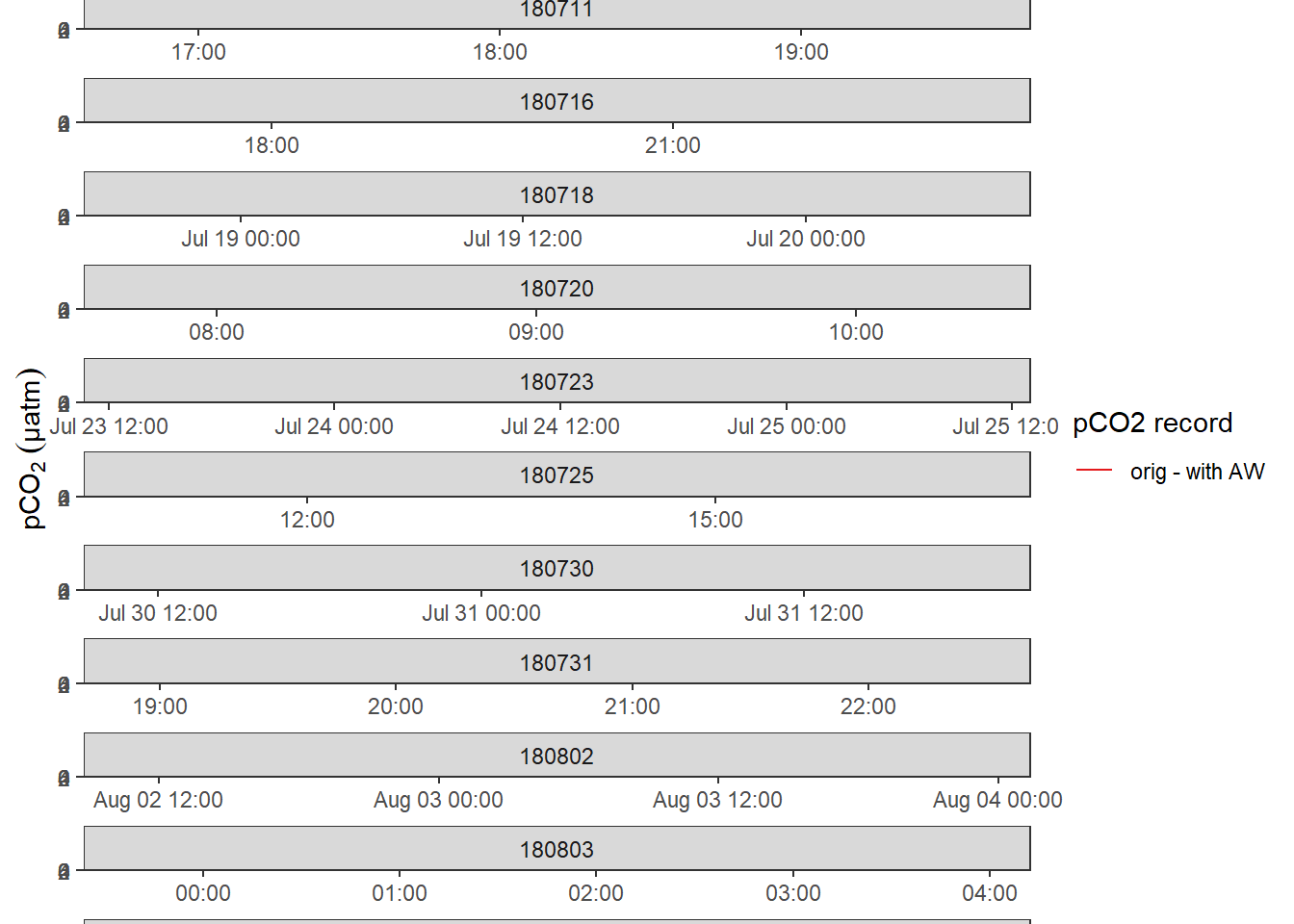
th_comparison %>%
  filter(!is.na(pCO2_corr)) %>%
  ggplot() +
  geom_path(aes(date_time, pCO2_withoutAW-pCO2_withAW, col = "without - with AW"))+
  scale_color_brewer(palette = "Set1", name = "pCO2 record")+
  labs(y=expression(pCO[2]~(µatm)), x="")+
  facet_wrap(~ID, scales = "free_x", ncol = 1)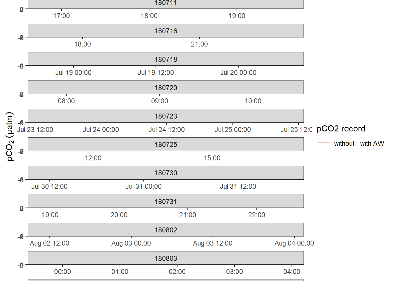
1.4.3 replace pCO2 data
th_new_withAW <- th_new_withAW %>%
  select(date_time, pCO2_corr)

ts_th <- ts_th %>%
  select(-pCO2_corr)


ts_th <- full_join(ts_th, th_new_withAW)

rm(th_new_withAW, th_new_withoutAW)
1.4.4 Offset analog vs post-processed pCO2
ts_th %>%
  filter(!is.na(pCO2_corr)) %>%
  ggplot()+
  geom_path(aes(date_time, pCO2_corr - pCO2_analog))+
  ylim(-30, 0)+
  labs(y=expression(pCO[2]~(µats_th)), x="")+
  facet_wrap(~ID, scales = "free_x", ncol = 1)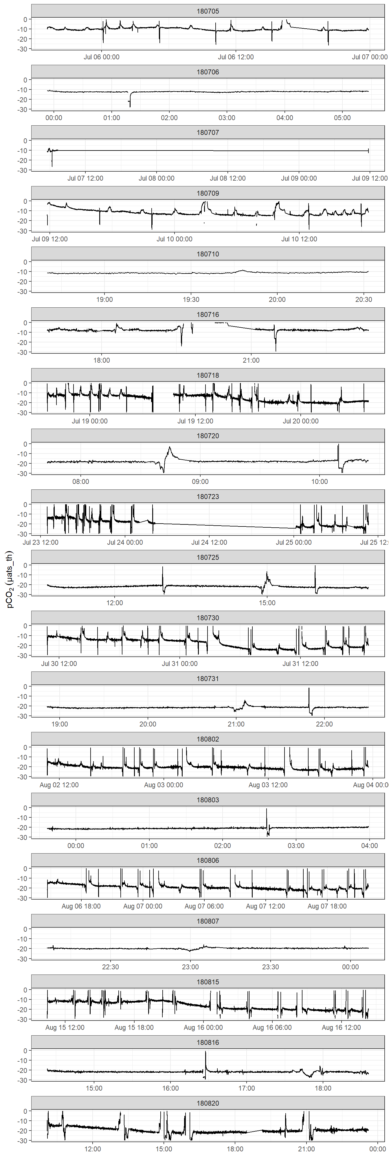
pCO2 difference betweeb HydroC and drift corrected data provided by Contos. Please note that pCO2 range is restricted to +/- 50 µatm.
2 Merges sensor (ts_th) + track (tt) data
ts_th <- read_csv(here::here("data/_merged_data_files/merging_interpolation",
                          "ts_th.csv"),
               col_types = cols(ID = col_character(),
                                pCO2_analog = col_double(),
                                pCO2_corr = col_double(),
                                Zero = col_factor(),
                                Flush = col_factor(),
                                Zero_counter = col_integer(),
                                deployment = col_integer(),
                                duration = col_double(),
                                mixing = col_character()))


tt <- read_csv(here::here("Data/_summarized_data_files",
                          "tt.csv"))


tm <- full_join(ts_th, tt) %>%
  arrange(date_time)

# interpolate tt data and than remove columns that originate from tt time stamp
tm <- tm %>%
  mutate(lat = approxfun(date_time, lat)(date_time),
         lon = approxfun(date_time, lon)(date_time)) %>%
  filter(!is.na(dep))

tm %>% write_csv(here::here("Data/_merged_data_files/merging_interpolation",
                            "tm.csv"))

rm(tm, ts_th, tt)
3 Tasks / open questions
sessionInfo()R version 4.0.2 (2020-06-22)
Platform: x86_64-w64-mingw32/x64 (64-bit)
Running under: Windows 10 x64 (build 18363)
Matrix products: default
locale:
[1] LC_COLLATE=English_Germany.1252 LC_CTYPE=English_Germany.1252
[3] LC_MONETARY=English_Germany.1252 LC_NUMERIC=C
[5] LC_TIME=English_Germany.1252
attached base packages:
[1] stats graphics grDevices utils datasets methods base
other attached packages:
[1] zoo_1.8-8 lubridate_1.7.9 forcats_0.5.0 stringr_1.4.0
[5] dplyr_1.0.0 purrr_0.3.4 readr_1.3.1 tidyr_1.1.0
[9] tibble_3.0.3 ggplot2_3.3.2 tidyverse_1.3.0 workflowr_1.6.2
loaded via a namespace (and not attached):
[1] Rcpp_1.0.5 here_0.1 lattice_0.20-41 assertthat_0.2.1
[5] rprojroot_1.3-2 digest_0.6.25 R6_2.4.1 cellranger_1.1.0
[9] backports_1.1.8 reprex_0.3.0 evaluate_0.14 highr_0.8
[13] httr_1.4.2 pillar_1.4.6 rlang_0.4.7 readxl_1.3.1
[17] rstudioapi_0.11 whisker_0.4 blob_1.2.1 rmarkdown_2.3
[21] labeling_0.3 munsell_0.5.0 broom_0.7.0 compiler_4.0.2
[25] httpuv_1.5.4 modelr_0.1.8 xfun_0.16 pkgconfig_2.0.3
[29] htmltools_0.5.0 tidyselect_1.1.0 fansi_0.4.1 crayon_1.3.4
[33] dbplyr_1.4.4 withr_2.2.0 later_1.1.0.1 grid_4.0.2
[37] jsonlite_1.7.0 gtable_0.3.0 lifecycle_0.2.0 DBI_1.1.0
[41] git2r_0.27.1 magrittr_1.5 scales_1.1.1 cli_2.0.2
[45] stringi_1.4.6 farver_2.0.3 fs_1.4.2 promises_1.1.1
[49] xml2_1.3.2 ellipsis_0.3.1 generics_0.0.2 vctrs_0.3.2
[53] RColorBrewer_1.1-2 tools_4.0.2 glue_1.4.1 hms_0.5.3
[57] yaml_2.2.1 colorspace_1.4-1 rvest_0.3.6 knitr_1.29
[61] haven_2.3.1