Response time correction of Contros HydroC pCO2 data
Jens Daniel Müller
14 November, 2019
Last updated: 2019-11-14
Checks: 7 0
Knit directory: BloomSail/
This reproducible R Markdown analysis was created with workflowr (version 1.4.0). The Checks tab describes the reproducibility checks that were applied when the results were created. The Past versions tab lists the development history.
Great! Since the R Markdown file has been committed to the Git repository, you know the exact version of the code that produced these results.
Great job! The global environment was empty. Objects defined in the global environment can affect the analysis in your R Markdown file in unknown ways. For reproduciblity it’s best to always run the code in an empty environment.
The command set.seed(20191021) was run prior to running the code in the R Markdown file. Setting a seed ensures that any results that rely on randomness, e.g. subsampling or permutations, are reproducible.
Great job! Recording the operating system, R version, and package versions is critical for reproducibility.
Nice! There were no cached chunks for this analysis, so you can be confident that you successfully produced the results during this run.
Great job! Using relative paths to the files within your workflowr project makes it easier to run your code on other machines.
Great! You are using Git for version control. Tracking code development and connecting the code version to the results is critical for reproducibility. The version displayed above was the version of the Git repository at the time these results were generated.
Note that you need to be careful to ensure that all relevant files for the analysis have been committed to Git prior to generating the results (you can use wflow_publish or wflow_git_commit). workflowr only checks the R Markdown file, but you know if there are other scripts or data files that it depends on. Below is the status of the Git repository when the results were generated:
Ignored files:
    Ignored:    .Rhistory
    Ignored:    .Rproj.user/
    Ignored:    data/TinaV/
    Ignored:    data/_merged_data_files/
    Ignored:    data/_summarized_data_files/

Untracked files:
    Untracked:  docs/reports/
Note that any generated files, e.g. HTML, png, CSS, etc., are not included in this status report because it is ok for generated content to have uncommitted changes.
These are the previous versions of the R Markdown and HTML files. If you’ve configured a remote Git repository (see ?wflow_git_remote), click on the hyperlinks in the table below to view them.
| File | Version | Author | Date | Message |
|---|---|---|---|---|
| html | d61a468 | jens-daniel-mueller | 2019-11-14 | Build site. |
| Rmd | 76e38c6 | jens-daniel-mueller | 2019-11-14 | rebuild site, new toc depth |
| html | 08b9a38 | jens-daniel-mueller | 2019-11-08 | Build site. |
| Rmd | ad4aa12 | jens-daniel-mueller | 2019-11-08 | Finalized RT determination |
| html | ad4aa12 | jens-daniel-mueller | 2019-11-08 | Finalized RT determination |
| html | b8dac9c | jens-daniel-mueller | 2019-11-08 | Build site. |
| Rmd | efcf0d6 | jens-daniel-mueller | 2019-11-08 | Finalized and cleaned RT determination |
| html | f3277a5 | jens-daniel-mueller | 2019-11-08 | Build site. |
| Rmd | aa27fd4 | jens-daniel-mueller | 2019-11-08 | Finalized RT determination |
| html | 4256bcf | jens-daniel-mueller | 2019-11-08 | Build site. |
| Rmd | 7f52e66 | jens-daniel-mueller | 2019-11-08 | response_time pdf updated |
| html | 72687ee | jens-daniel-mueller | 2019-11-08 | Build site. |
| Rmd | 74632d6 | jens-daniel-mueller | 2019-11-08 | response_time pdf updated |
| html | 74212a6 | jens-daniel-mueller | 2019-11-08 | Build site. |
| Rmd | 6cb1935 | jens-daniel-mueller | 2019-11-08 | response_time updated |
| html | 33e3659 | jens-daniel-mueller | 2019-10-22 | Build site. |
| Rmd | efcafd1 | jens-daniel-mueller | 2019-10-22 | Added data base, merging, and RT determination |
| html | 1595fe9 | jens-daniel-mueller | 2019-10-21 | Build site. |
| html | a059c41 | jens-daniel-mueller | 2019-10-21 | Build site. |
| Rmd | eff54ce | jens-daniel-mueller | 2019-10-21 | Added CTD read-in |
| html | 32ec4f7 | jens-daniel-mueller | 2019-10-21 | Build site. |
| Rmd | b2d2bbb | jens-daniel-mueller | 2019-10-21 | Structured data base and response time Rmd |
| html | bafa88f | jens-daniel-mueller | 2019-10-21 | Build site. |
| Rmd | 53ad162 | jens-daniel-mueller | 2019-10-21 | Structured data base and response time Rmd |
| html | 076a36b | jens-daniel-mueller | 2019-10-21 | Build site. |
| Rmd | 3e8a32e | jens-daniel-mueller | 2019-10-21 | Structured data base and response time Rmd |
| html | b2d0164 | jens-daniel-mueller | 2019-10-21 | Build site. |
| Rmd | 53ae361 | jens-daniel-mueller | 2019-10-21 | Added data base and response time Rmd |
library(tidyverse)
library(seacarb)
library(data.table)
library(broom)
library(lubridate)
Sensitivity considerations
A change in DIC of 1 µmol kg-1 corresponds to a change in pCO2 of around 1 µatm, in the Central Baltic Sea at a pCO2 of around 100 µatm (summertime conditions).
df <- data.frame(cbind(
  (c(1720)),
  (c(7))))

Tem <- seq(5,25,5)
pCO2<-seq(50,500,20)

df<-merge(df, Tem)
names(df) <- c("AT", "S", "Tem")

df<-merge(df, pCO2)
names(df) <- c("AT", "S", "Tem", "pCO2")

df<-data.table(df)
df$AT<-df$AT*1e-6

df$DIC<-carb(flag=24, var1=df$pCO2, var2=df$AT, S=df$S, T=df$Tem, k1k2="m10", kf="dg", pHscale="T")[,16]
df$pCO2.corr<-carb(flag=15, var1=df$AT, var2=df$DIC, S=df$S, T=df$Tem, k1k2="m10", kf="dg", pHscale="T")[,9]

df$pCO2.2<-df$pCO2.corr + 25
df$DIC.2<-carb(flag=24, var1=df$pCO2.2, var2=df$AT, S=df$S, T=df$Tem, k1k2="m10", kf="dg", pHscale="T")[,16]


df$ratio<-(df$pCO2.2-df$pCO2.corr)/(df$DIC.2*1e6-df$DIC*1e6)

df %>%
  ggplot(aes(pCO2, ratio, col=as.factor(Tem)))+
  geom_line()+
  scale_color_viridis_d(option = "C",name="Tem [°C]")+
  labs(x=expression(pCO[2]~(µatm)), y=expression(Delta~pCO[2]~"/"~Delta~DIC~(µatm~µmol^{-1}~kg)))+
  scale_y_continuous(limits = c(0,8), breaks = seq(0,10,1))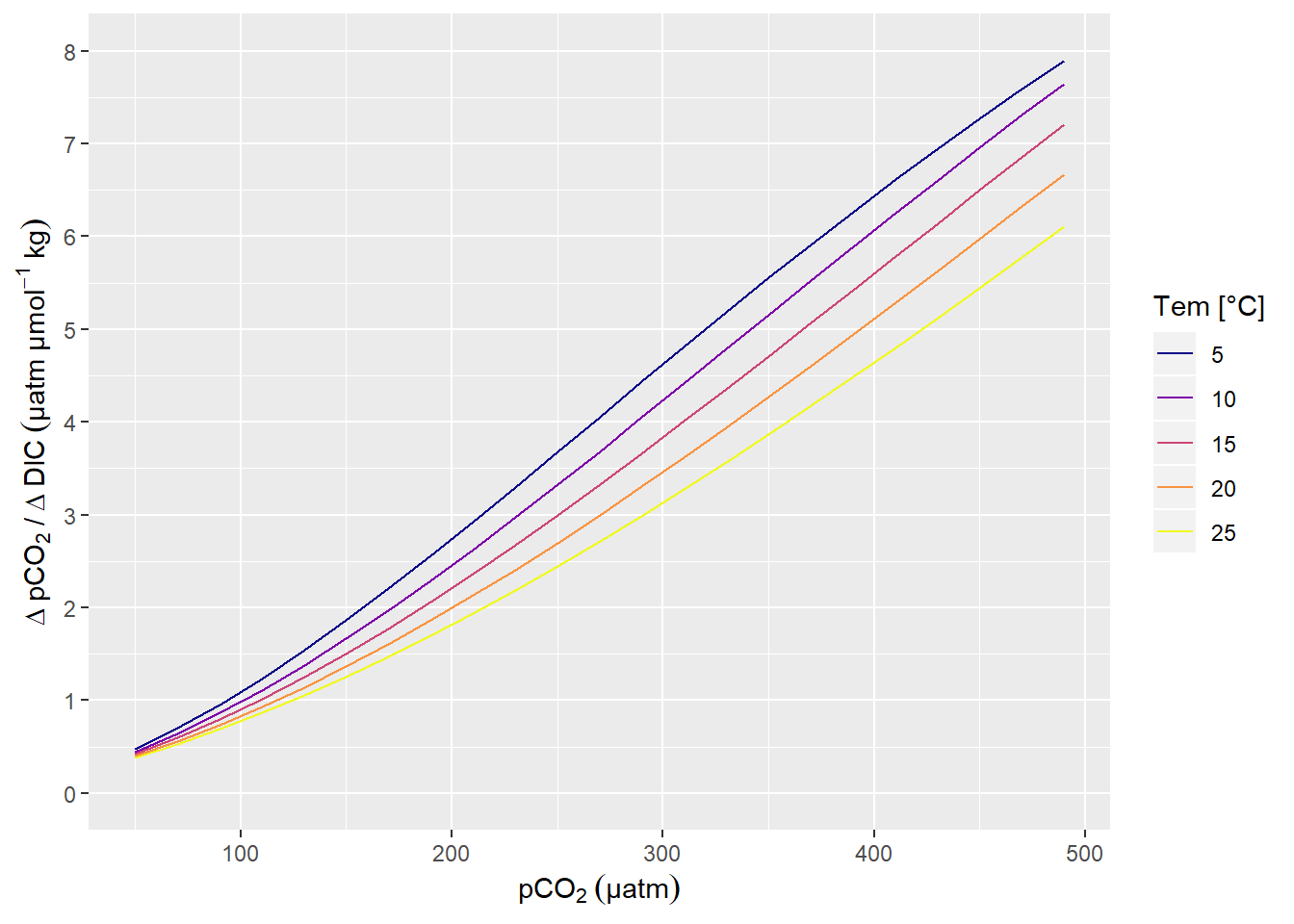
pCO2 sensitivity to changes in DIC.
| Version | Author | Date |
|---|---|---|
| 33e3659 | jens-daniel-mueller | 2019-10-22 |
rm(df, Tem, pCO2)Response time determination
HydroC sensor settings
The sensor was first run with a low power pump (1W). Later - and for most parts of the expedition - with a stronger (8W) pump. Pumps were switched between recordings (data file: SD_datafile_20180718_170417CO2-0618-001.txt):
- 2018-07-17;13:08:34
- 2018-07-17;13:08:35
Logging frequency for all measurement modes (Measure, Zero, Flush) was increased in two steps, It was:
10 sec for all recordings including SD_datafile_20180714_073641CO2-0618-001.txt
2 sec after change in SD_datafile_20180717_121052CO2-0618-001.txt at:
- 2018-07-14;07:52:02
- 2018-07-14;07:52:12
- 2018-07-14;07:52:14
1 sec after change in SD_datafile_20180718_170417CO2-0618-001 at:
- 2018-07-17;12:27:25
- 2018-07-17;12:27:27
- 2018-07-17;12:27:28
Model fitting
Response times were determined by fitting a nonlinear least-squares model with the nls function as described here by Douglas Watson.
- Flush period length: variable
- Flush period restricted to equilibration phase, avoiding initial gas mixing effects occuring at the start of each Flush period
- only completed Flush periods (duration > 500 sec) included
df <- read_csv(here::here("data/_merged_data_files",
                          "BloomSail_CTD_HydroC_Contros_clean.csv"),
               col_types = cols(ID = col_character(),
                                pCO2_analog = col_double(),
                                pCO2 = col_double(),
                                Zero = col_factor(),
                                Flush = col_factor(),
                                Zero_ID = col_integer(),
                                duration = col_double(),
                                mixing = col_character()))

df <- df %>%
  select(date_time, ID, dep, tem, Flush, pCO2, Zero_ID, duration, mixing)

df <- df %>%
  filter(Flush == 1, mixing == "equilibration")

df <- df %>%
  group_by(Zero_ID) %>%
  mutate(duration = duration- min(duration),
         max_duration = max(duration)) %>%
  ungroup() %>%
  filter(max_duration >= 500) %>%
  select(-max_duration)
An example plot for a nls model fitted to pCO2 observations during a Flush phase is shown below.
i <- 95

df_ID <- df %>%
  filter(Zero_ID == i, duration <= 300)

fit <-
df_ID %>%
  nls(pCO2 ~ SSasymp(duration, yf, y0, log_alpha), data = .)

tau <- as.numeric(exp(-tidy(fit)[3,2]))
pCO2_end <- as.numeric(tidy(fit)[1,2])
pCO2_start <- as.numeric(tidy(fit)[2,2])
dpCO2 = pCO2_end - pCO2_start
mean_abs_resid <- mean(abs(resid(fit)))

augment(fit) %>%
  ggplot(aes(duration, pCO2))+
  geom_point()+
  geom_line(aes(y = .fitted))+
  geom_vline(xintercept = tau)+
  geom_hline(yintercept = pCO2_start + 0.63 *(dpCO2))+
  labs(y=expression(pCO[2]~(µatm)), x="Duration of Flush period (s)")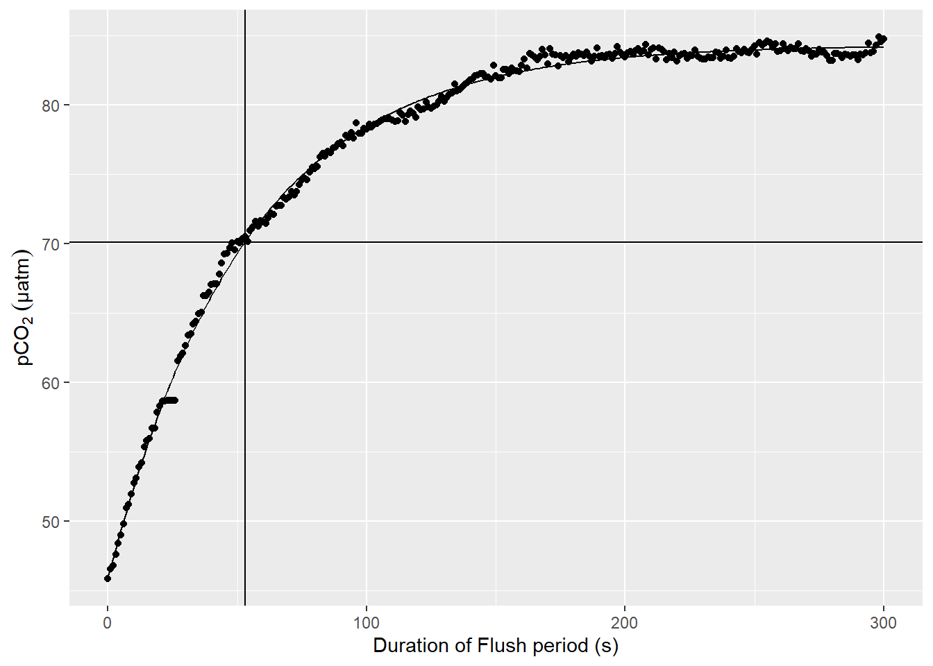
Example response time determination by non-linear least squares fit to the pCO2 recovery signal after zeroing. The vertical line indicates the determined response time tau. The horizontal line indicates 63% of the difference between start and final fitted pCO2.
| Version | Author | Date |
|---|---|---|
| 74212a6 | jens-daniel-mueller | 2019-11-08 |
rm(df_ID, fit, i, tau, dpCO2, pCO2_end, pCO2_start)duration_intervals <- seq(150,500,50)As there was some speculation about the dependence of determined response times (\(\tau\)) on the chosen duration of the fit interval, the response time \(\tau\) was determined for all zeroings and for total durations of:
150, 200, 250, 300, 350, 400, 450, 500 secs
# Plot all individual Flush periods with exponential fit ----------------------

pdf(file=here::here("output/Plots/response_time",
    "RT_determination.pdf"), onefile = TRUE, width = 7, height = 4)

for (i in unique(df$Zero_ID)) {
  for (max_duration in duration_intervals) {

    df_ID <- df %>%
      filter(Zero_ID == i, duration <= max_duration)

    fit <-
      try(
      df_ID %>%
          nls(pCO2 ~ SSasymp(duration, yf, y0, log_alpha), data = .),
      TRUE)

    if (class(fit) == "nls"){

      tau <- as.numeric(exp(-tidy(fit)[3,2]))
      pCO2_end <- as.numeric(tidy(fit)[1,2])
      pCO2_start <- as.numeric(tidy(fit)[2,2])
      dpCO2 = pCO2_end - pCO2_start
      mean_abs_resid <- mean(abs(resid(fit))/pCO2_end)*100

      temp <- as_tibble(bind_cols(Zero_ID = i, duration = max_duration, tau = tau, resid = mean_abs_resid))

      if (exists("tau_df")){tau_df <- bind_rows(tau_df, temp)}
        else {tau_df <- temp}

      if (mean_abs_resid > 1){warn <- "orange"}
        else {warn <- "black"}

      print(
      augment(fit) %>%
        ggplot(aes(duration, pCO2))+
        geom_point(col = warn)+
        geom_line(aes(y = .fitted))+
        geom_vline(xintercept = tau)+
        geom_hline(yintercept = pCO2_start + 0.63 *(dpCO2))+
        labs(y=expression(pCO[2]~(µatm)), x="Duration of Flush period (s)",
             title = paste("Zero_ID: ", i,
                           "Tau: ", round(tau,1),
                           "Mean absolute residual (%): ", round(mean_abs_resid, 2)))+
        xlim(0,600)
      )

    }


    else {

      temp <- as_tibble(bind_cols(Zero_ID = i, duration = max_duration, tau = NaN, resid = NaN))

      if (exists("tau_df")){tau_df <- bind_rows(tau_df, temp)}
        else {tau_df <- temp}

      print(
      df_ID %>%
        ggplot(aes(duration, pCO2))+
        geom_point(col="red")+
        labs(y=expression(pCO[2]~(µatm)), x="Duration of Flush period (s)",
             title = paste("Zero_ID: ", i,
                           "nls model failed"))+
        xlim(0,600)
      )

    }
  }
}

dev.off()

rm(df_ID, fit, i, tau, dpCO2, pCO2_end, pCO2_start, temp, max_duration, mean_abs_resid, warn)

tau_df %>%
  write_csv(here::here("data/_summarized_data_files", "Tina_V_HydroC_response_times_all.csv"))

# Plot individual Flush periods with linearized response variable  --------
# for (i in unique(df$Zero_ID)) {
#
# #i <- 50
# df_ID <- df %>%
#   filter(Zero_ID == i,
#          mixing == "equilibration")
#
# mean_pCO2 <- df_ID %>%
#   slice((n()-4) : n()) %>%
#   summarise(mean_pCO2 = mean(pCO2))
#
# df_ID <- full_join(df_ID, mean_pCO2) %>%
#   mutate(dpCO2 = max(pCO2) - pCO2,
#          ln_dpCO2 = log(dpCO2))
#
#
# df_ID %>%
#   ggplot(aes(duration_equi, ln_dpCO2))+
#   geom_point()+
#   geom_smooth(method = "lm")+
#   theme_bw()
#
# # augment(fit) %>%
# #   ggplot(aes(duration_equi, pCO2))+
# #   geom_point()+
# #   geom_line(aes(y = .fitted))+
# #   geom_vline(xintercept = tau)
#
# ggsave(here::here("/Plots/TinaV/Sensor/HydroC_diagnostics/Response_time_fits",
#                   paste(i,"_Zero_ID_HydroC_RT_linear.jpg", sep="")),
#          width = 10, height = 4)
# }
A pdf with plots of all individual response time fits can be accessed here
Outcome
General cosiderations
Estimated \(\tau\) values were only taken into account when stable environmental pCO2 levels were present. Absence of stable environmental pCO2 was assumed when the mean absolute fit residual was above 1 % of the final equilibrium pCO2. If one model fit (irrespective the chosen fit interval length) of a particular flush period did not match that criterion, the flush period was ignored. Usually, fits with the higher duration did not meet this criterion. For some unexplained reason the first \(\tau\) determination resulted in values about twice as high as all other Flush periods and was therefore removed as an outlier.
Metrics to characterize the fitting procedure include the number of:
- Flush periods: 55
- Duration intervals: 8
- Exercised response time fits: 440
- Succesful response times determinations: 417 (94.8)%
- \(\tau\)’s after removing groups of fits with high absolute fit residual: 296 (67.3 %)
It should be noted that all failed model fits occured in flush periods where the residual criterion was not meet by at least one other fit (i.e. fitting only failed under unstable conditions).
tau_df %>%
  ggplot(aes(resid))+
  geom_histogram()+
  facet_wrap(~duration, labeller = label_both)+
  geom_vline(xintercept = resid_limit)+
  labs(x=expression(Mean~absolute~residuals~("%"~of~equilibrium~pCO[2])))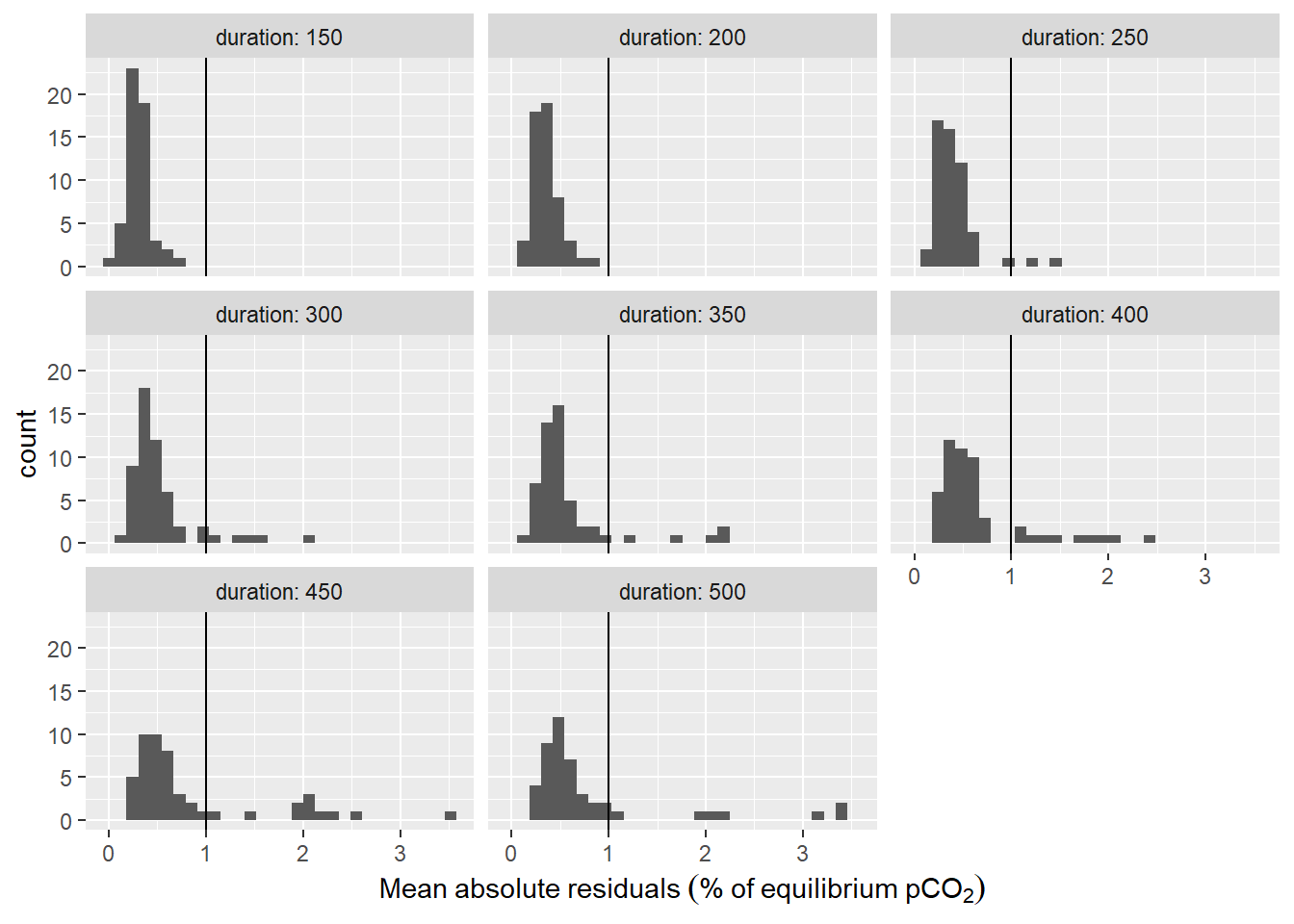
Histogram of residuals from fit displayed for the investigate durations of the fit interval. Vertical line represents the chosen threshold.
| Version | Author | Date |
|---|---|---|
| f3277a5 | jens-daniel-mueller | 2019-11-08 |
tau_resid %>%
  ggplot(aes(Zero_ID, tau, col=duration))+
  geom_point()+
  scale_color_viridis_c(name="Duration (sec)")+
  labs(y="Tau (sec)")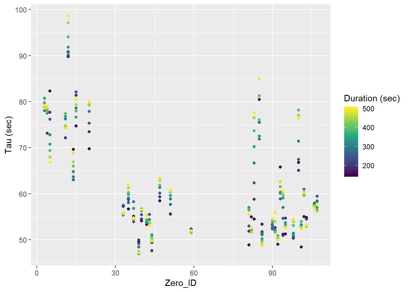
Tau for all Zeroings with color representing the fit interval duration.
Fit interval length
tau_resid %>%
  group_by(Zero_ID) %>%
  mutate(d_tau = tau - mean(tau)) %>%
  ggplot(aes(duration, d_tau))+
  geom_hline(yintercept = 0)+
  geom_smooth()+
  geom_point()+
  facet_wrap(~Zero_ID, ncol = 4, labeller = label_both)+
  labs(x="Duration (sec)", y="Deviation from mean tau (sec)")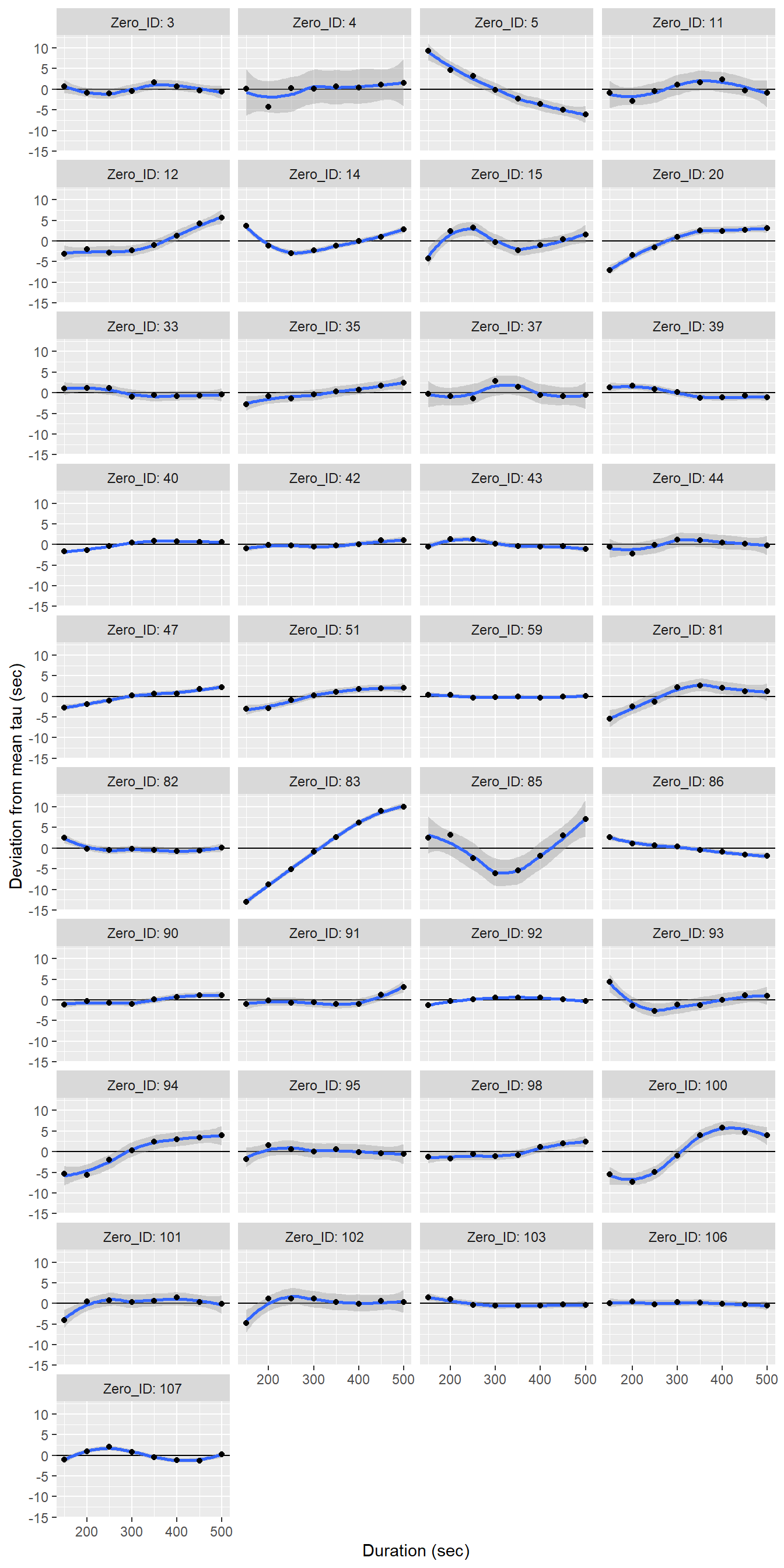
Determined tau values as a function of the fit interval duration, displayed individually for each flush period.
tau_resid %>%
  group_by(Zero_ID) %>%
  mutate(d_tau = tau - mean(tau)) %>%
  ggplot(aes(duration, d_tau))+
  geom_violin(aes(group=duration))+
  geom_point()+
  labs(x="Duration (sec)", y="Deviation from mean tau (sec)")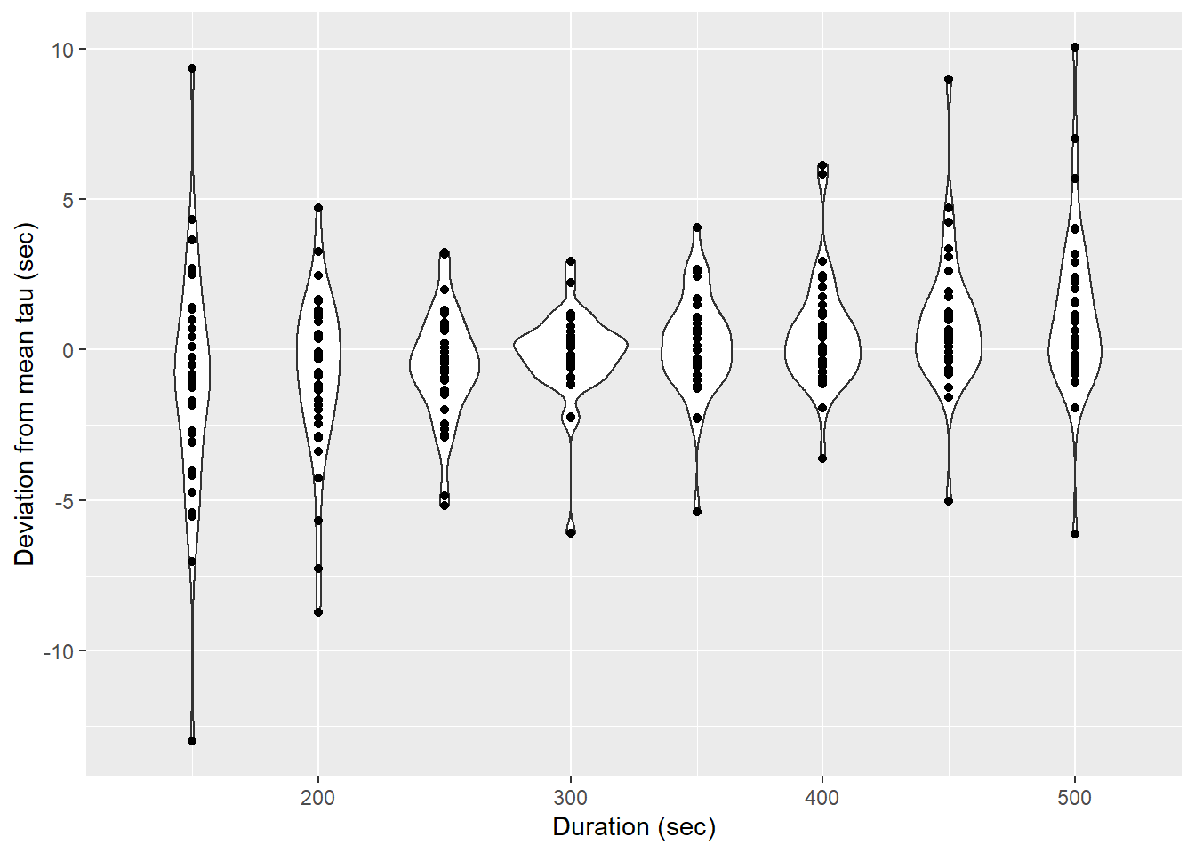
Determined tau values as a function of the fit interval duration, pooled for all flush period.
Mean response time
Finally, the mean response times are:
max_Zero_ID <- max(unique(df[df$date_time < ymd_hms("2018-07-17;13:08:34"),]$Zero_ID))
min_Zero_ID <- min(unique(df[df$date_time > ymd_hms("2018-07-17;13:08:34"),]$Zero_ID))

# tau_df %>%
#   mutate(pump_power = if_else(Zero_ID <= 20, "1W", "8W")) %>%
#   group_by(pump_power) %>%
#   summarise(tau = mean(tau, na.rm = TRUE))

tau_final <- tau_resid %>%
  mutate(pump_power = if_else(Zero_ID <= max_Zero_ID, "1W", "8W")) %>%
  group_by(pump_power) %>%
  summarise(tau = mean(tau))

tau_final
# A tibble: 2 x 2
pump_power tau
<chr> <dbl>
1 1W 77.4
2 8W 56.6rm(list=setdiff(ls(), "tau_final"))Response time correction
Pre-smoothing
Response time correction
Post-smoothing
Response time optimization
Open tasks / questions
- Compare Contros and own response time estimates
- Compare differnt response time correction methods (Bittig vs. Fiedler, Miloshevich, Fietzek)
- Check results from field response time experiment (high zeroing frequency)
sessionInfo()R version 3.5.0 (2018-04-23)
Platform: x86_64-w64-mingw32/x64 (64-bit)
Running under: Windows 10 x64 (build 17763)
Matrix products: default
locale:
[1] LC_COLLATE=English_United States.1252
[2] LC_CTYPE=English_United States.1252
[3] LC_MONETARY=English_United States.1252
[4] LC_NUMERIC=C
[5] LC_TIME=English_United States.1252
attached base packages:
[1] stats graphics grDevices utils datasets methods base
other attached packages:
[1] lubridate_1.7.4 broom_0.5.2 data.table_1.12.6
[4] seacarb_3.2.12 oce_1.1-1 gsw_1.0-5
[7] testthat_2.2.1 forcats_0.4.0 stringr_1.4.0
[10] dplyr_0.8.3 purrr_0.3.3 readr_1.3.1
[13] tidyr_1.0.0 tibble_2.1.3 ggplot2_3.2.1
[16] tidyverse_1.2.1
loaded via a namespace (and not attached):
[1] tidyselect_0.2.5 xfun_0.10 haven_2.1.1
[4] lattice_0.20-35 colorspace_1.4-1 vctrs_0.2.0
[7] generics_0.0.2 viridisLite_0.3.0 htmltools_0.4.0
[10] yaml_2.2.0 utf8_1.1.4 rlang_0.4.1
[13] pillar_1.4.2 glue_1.3.1 withr_2.1.2
[16] modelr_0.1.5 readxl_1.3.1 lifecycle_0.1.0
[19] munsell_0.5.0 gtable_0.3.0 workflowr_1.4.0
[22] cellranger_1.1.0 rvest_0.3.4 evaluate_0.14
[25] labeling_0.3 knitr_1.25 fansi_0.4.0
[28] highr_0.8 Rcpp_1.0.2 scales_1.0.0
[31] backports_1.1.5 jsonlite_1.6 fs_1.3.1
[34] hms_0.5.1 digest_0.6.22 stringi_1.4.3
[37] grid_3.5.0 rprojroot_1.3-2 here_0.1
[40] cli_1.1.0 tools_3.5.0 magrittr_1.5
[43] lazyeval_0.2.2 crayon_1.3.4 whisker_0.4
[46] pkgconfig_2.0.3 zeallot_0.1.0 xml2_1.2.2
[49] assertthat_0.2.1 rmarkdown_1.16 httr_1.4.1
[52] rstudioapi_0.10 R6_2.4.0 nlme_3.1-137
[55] git2r_0.26.1 compiler_3.5.0