World Ocean Atlas 2018
Jens Daniel Müller
11 August, 2020
Last updated: 2020-08-11
Checks: 7 0
Knit directory: Cant_eMLR/
This reproducible R Markdown analysis was created with workflowr (version 1.6.2). The Checks tab describes the reproducibility checks that were applied when the results were created. The Past versions tab lists the development history.
Great! Since the R Markdown file has been committed to the Git repository, you know the exact version of the code that produced these results.
Great job! The global environment was empty. Objects defined in the global environment can affect the analysis in your R Markdown file in unknown ways. For reproduciblity it’s best to always run the code in an empty environment.
The command set.seed(20200707) was run prior to running the code in the R Markdown file. Setting a seed ensures that any results that rely on randomness, e.g. subsampling or permutations, are reproducible.
Great job! Recording the operating system, R version, and package versions is critical for reproducibility.
Nice! There were no cached chunks for this analysis, so you can be confident that you successfully produced the results during this run.
Great job! Using relative paths to the files within your workflowr project makes it easier to run your code on other machines.
Great! You are using Git for version control. Tracking code development and connecting the code version to the results is critical for reproducibility.
The results in this page were generated with repository version 5d45981. See the Past versions tab to see a history of the changes made to the R Markdown and HTML files.
Note that you need to be careful to ensure that all relevant files for the analysis have been committed to Git prior to generating the results (you can use wflow_publish or wflow_git_commit). workflowr only checks the R Markdown file, but you know if there are other scripts or data files that it depends on. Below is the status of the Git repository when the results were generated:
Ignored files:
    Ignored:    .Rproj.user/
    Ignored:    analysis/figure/
    Ignored:    data/GLODAPv1_1/
    Ignored:    data/GLODAPv2_2016b_MappedClimatologies/
    Ignored:    data/GLODAPv2_2020/
    Ignored:    data/Gruber_2019/
    Ignored:    data/WOCE/
    Ignored:    data/World_Ocean_Atlas_2018/
    Ignored:    data/dclement/
    Ignored:    data/eMLR/
    Ignored:    data/pCO2_atmosphere/
    Ignored:    data/parameters/
    Ignored:    dump/

Untracked files:
    Untracked:  analysis/python_scripts/
    Untracked:  code/plotting_functions.R
    Untracked:  code/test_scripts/
    Untracked:  figure/
Note that any generated files, e.g. HTML, png, CSS, etc., are not included in this status report because it is ok for generated content to have uncommitted changes.
These are the previous versions of the repository in which changes were made to the R Markdown (analysis/read_World_Ocean_Atlas_2018.Rmd) and HTML (docs/read_World_Ocean_Atlas_2018.html) files. If you’ve configured a remote Git repository (see ?wflow_git_remote), click on the hyperlinks in the table below to view the files as they were in that past version.
| File | Version | Author | Date | Message |
|---|---|---|---|---|
| Rmd | 5d45981 | jens-daniel-mueller | 2020-08-11 | plot sal sections from function both basins |
| html | 495debb | jens-daniel-mueller | 2020-08-11 | Build site. |
| Rmd | cfbc5e4 | jens-daniel-mueller | 2020-08-11 | plot sections from function both basins |
| html | 075099b | jens-daniel-mueller | 2020-08-11 | Build site. |
| Rmd | adc0335 | jens-daniel-mueller | 2020-08-11 | plot sections from function |
| Rmd | 69b9a78 | jens-daniel-mueller | 2020-08-11 | plot sections from function |
| html | cfd84b7 | jens-daniel-mueller | 2020-08-11 | Build site. |
| Rmd | ca836af | jens-daniel-mueller | 2020-08-11 | Removed Rmd child tests |
| html | dc2b649 | jens-daniel-mueller | 2020-08-11 | Build site. |
| Rmd | 928cd7d | jens-daniel-mueller | 2020-08-11 | Rmd child test with access to global object |
| html | be47191 | jens-daniel-mueller | 2020-08-11 | Build site. |
| Rmd | 9c8f6b8 | jens-daniel-mueller | 2020-08-11 | Rmd child test with variable name transmission |
| html | 6ebb3de | jens-daniel-mueller | 2020-08-11 | Build site. |
| Rmd | 0333c99 | jens-daniel-mueller | 2020-08-11 | test addition child Rmd file |
| html | fbbabf4 | jens-daniel-mueller | 2020-08-11 | Build site. |
| Rmd | e92638d | jens-daniel-mueller | 2020-08-11 | plot maps from function |
| html | cee0e89 | jens-daniel-mueller | 2020-08-11 | Build site. |
| Rmd | c9e2d65 | jens-daniel-mueller | 2020-08-11 | plot maps from function |
| html | de933d9 | jens-daniel-mueller | 2020-08-11 | Build site. |
| Rmd | c3a6c63 | jens-daniel-mueller | 2020-08-11 | included WOA land mask and longitude conversion |
| html | 5d33341 | jens-daniel-mueller | 2020-08-11 | Build site. |
| html | 8a010ca | jens-daniel-mueller | 2020-08-11 | Build site. |
| html | a01041a | jens-daniel-mueller | 2020-08-11 | Build site. |
| html | e18e59a | jens-daniel-mueller | 2020-08-10 | Build site. |
| html | 7d7900a | jens-daniel-mueller | 2020-08-07 | Build site. |
| html | 4394942 | jens-daniel-mueller | 2020-08-04 | Build site. |
| Rmd | eb838d4 | jens-daniel-mueller | 2020-08-04 | Read, plot, write data from D Clement |
| html | 662560f | jens-daniel-mueller | 2020-08-04 | Build site. |
| Rmd | b2b1f24 | jens-daniel-mueller | 2020-08-04 | Read, plot, write data from D Clement |
| html | e9a52c5 | jens-daniel-mueller | 2020-07-31 | Build site. |
| Rmd | 5ee70b2 | jens-daniel-mueller | 2020-07-31 | formatting |
| html | f33772b | jens-daniel-mueller | 2020-07-31 | Build site. |
| Rmd | dea0eaf | jens-daniel-mueller | 2020-07-31 | alligned plots with GLODAP climatology |
| html | 9dc5d7f | jens-daniel-mueller | 2020-07-29 | Build site. |
| html | 21524b4 | jens-daniel-mueller | 2020-07-29 | Build site. |
| html | f5c4667 | jens-daniel-mueller | 2020-07-29 | Build site. |
| Rmd | f6d4d92 | jens-daniel-mueller | 2020-07-29 | format and plots revised |
| html | 8d71a56 | jens-daniel-mueller | 2020-07-29 | Build site. |
| Rmd | 82db969 | jens-daniel-mueller | 2020-07-29 | format and plots revised |
| html | 2e08795 | jens-daniel-mueller | 2020-07-24 | Build site. |
| html | 61a1a48 | jens-daniel-mueller | 2020-07-24 | Build site. |
| Rmd | 864a6e3 | jens-daniel-mueller | 2020-07-24 | merged predictor data sets |
| html | eb716ce | jens-daniel-mueller | 2020-07-23 | Build site. |
| Rmd | ffd46da | jens-daniel-mueller | 2020-07-23 | WOA18 read in |
| html | 556e6cc | jens-daniel-mueller | 2020-07-23 | Build site. |
| html | c1289a2 | jens-daniel-mueller | 2020-07-23 | Build site. |
| html | 2890e73 | jens-daniel-mueller | 2020-07-23 | Build site. |
| html | fdfa7b9 | jens-daniel-mueller | 2020-07-22 | Build site. |
| html | bb9c002 | jens-daniel-mueller | 2020-07-21 | Build site. |
| Rmd | d2ed0f8 | jens-daniel-mueller | 2020-07-21 | harmonied lat lon labeling |
| html | 97dbf5b | jens-daniel-mueller | 2020-07-21 | Build site. |
| Rmd | 5def7e8 | jens-daniel-mueller | 2020-07-21 | create csvs for each parameter |
| html | b47adc2 | jens-daniel-mueller | 2020-07-20 | Build site. |
| Rmd | 366d7d5 | jens-daniel-mueller | 2020-07-20 | update plots |
| html | 1de1bc0 | jens-daniel-mueller | 2020-07-20 | Build site. |
| Rmd | 68e4615 | jens-daniel-mueller | 2020-07-20 | assigned ocean basins and plotted world map |
| html | 3149ffd | jens-daniel-mueller | 2020-07-20 | Build site. |
| Rmd | 918f8c8 | jens-daniel-mueller | 2020-07-20 | assigned ocean basins and plotted world map |
| html | 2fa2896 | jens-daniel-mueller | 2020-07-20 | Build site. |
| Rmd | 23220a8 | jens-daniel-mueller | 2020-07-20 | assigned ocean basins and plotted world map |
| html | 27d380d | jens-daniel-mueller | 2020-07-20 | Build site. |
| Rmd | 09f3f73 | jens-daniel-mueller | 2020-07-20 | basin masks read in |
| html | 22b588c | jens-daniel-mueller | 2020-07-18 | Build site. |
| Rmd | 87a4680 | jens-daniel-mueller | 2020-07-18 | added WOA blank script |
library(tidyverse)
library(lubridate)
library(tidync)
library(stars)
1 Data source
- Data source: World Ocean Atlas 2018
2 Masks
2.1 Basins
2.1.1 Read mask
The surface mask (0m) with 1x1° resolution from the file basinmask_01.msk was used.
basinmask_01 <- read_csv(here::here("data/World_Ocean_Atlas_2018",
                                    "basinmask_01.msk"),
                         skip = 1,
                         col_types = list(.default = "d"))

basinmask_01 <- basinmask_01 %>%
  select(Latitude:Basin_0m) %>%
  mutate(Basin_0m = as.factor(Basin_0m)) %>%
  rename(lat = Latitude, lon = Longitude)
2.1.2 Labels
According to WOA FAQ website, number codes in the mask file refer to Ocean basins as follows:
- 1: Atlantic Ocean (with 10 - Southern Ocean, between 63°W and 20°E)
- 2: Pacific Ocean (with 10 - Southern Ocean, between 147°E and 63°W)
- 3: Indian Ocean (with 10 - Southern Ocean, between 20°E and 147°E)
From this, the Atlantik and the Indo-Pacific were labeled.
basinmask_01 <- basinmask_01 %>%
  filter(Basin_0m %in% c("1", "2", "3", "10")) %>%
  mutate(basin = if_else(Basin_0m == "10" & lon >= -63 & lon < 20,
                         "Atlantic", "Indo-Pacific"),
         basin = if_else(Basin_0m == "1",
                         "Atlantic", basin)) %>%
  select(-Basin_0m) %>%
  mutate(lon = if_else(lon < 20, lon + 360, lon))
2.2 Land
2.2.1 Read mask
The land sea mask with 1x1° resolution from the file landsea_01.msk was used.
landsea_01 <- read_csv(here::here("data/World_Ocean_Atlas_2018",
                                  "landsea_01.msk"),
                         skip = 1,
                         col_types = list(.default = "d"))

landmask <- landsea_01 %>%
  filter(Bottom_Standard_Level == 1) %>%
  select(-Bottom_Standard_Level)

landmask <- landmask %>%
  rename(lat = Latitude,
         lon = Longitude) %>%
  mutate(lon = if_else(lon < 20, lon + 360, lon))

rm(landsea_01)
2.2.2 Label
According to the WOA18 documentation document: “The landsea_XX.msk contains the standard depth level number at which the bottom of the ocean is first encountered at each quarter-degree or one-degree square for the entire world. Land will have a value of 1, corresponding to the surface.”
The landmask was derived as coordinates with value 1.
2.3 Plot map
ggplot() +
  geom_raster(data = landmask,
              aes(lon, lat), fill = "grey80") +
  geom_raster(data = basinmask_01,
              aes(lon, lat, fill = basin)) +
  scale_fill_brewer(palette = "Dark2") +
  coord_quickmap(expand = 0) +
  theme(legend.position = "top",
        legend.title = element_blank())
2.4 Write files
basinmask_01 %>%
  write_csv(here::here("data/World_Ocean_Atlas_2018/_summarized_files",
                       "basin_mask_WOA18.csv"))

landmask %>%
  write_csv(here::here("data/World_Ocean_Atlas_2018/_summarized_files",
                       "land_mask_WOA18.csv"))

rm(basinmask_01)
3 WOA18 data
Copied from the WOA FAQ website, the file naming conventions is:
PREF_DDDD_VTTFFGG.EXT, where:
- PREF: prefix
- DDDD: decade
- V: variable
- TT: time period
- FF: field type
- GG: grid (5deg- 5°, 01- 1°, 04 - 1/4°)
- EXT: file extention
Short description of the statistical fields in WOA
- Objectively analyzed climatologies are the objectively interpolated mean fields for oceanographic variables at standard - depth levels for the World Ocean.
- The statistical mean is the average of all unflagged interpolated values at each standard depth level for each variable - in each 1° square which contains at least one measurement for the given oceanographic variable.
- The number of observations of each variable in each 1° square of the World Ocean at each standard depth level.
- The standard deviation about the statistical mean of each variable in each 1° square at each standard depth level.
- The standard error of the mean of each variable in each 1° square at each standard depth level.
- The seasonal or monthly climatology minus the annual climatology at each 1° square at each standard depth.
- The statistical mean minus the climatological mean at each 1° square at each standard depth. This value is used as an estimate of interpolation and smoothing error.
- The number of 1° squares within the smallest radius of influence around each 1° square which contain a statistical mean.
Here, we use
- Fields: objectively analyzed mean
- Decades: all decades
- Grid: 1 deg resolution
3.1 Read ncdfs
# temperature

WOA_tem <- tidync(here::here("data/World_Ocean_Atlas_2018",
                                 "woa18_decav_t00_01.nc"))

WOA_tem_tibble <- WOA_tem %>% hyper_tibble()

WOA_tem_tibble <- WOA_tem_tibble  %>%
  select(tem = t_an, lon, lat, depth) %>%
  drop_na() %>%
  mutate(lon = if_else(lon < 20, lon + 360, lon))

# salinity

WOA_sal <- tidync(here::here("data/World_Ocean_Atlas_2018",
                                 "woa18_decav_s00_01.nc"))

WOA_sal_tibble <- WOA_sal %>% hyper_tibble()

WOA_sal_tibble <- WOA_sal_tibble  %>%
  select(sal = s_an, lon, lat, depth) %>%
  drop_na() %>%
  mutate(lon = if_else(lon < 20, lon + 360, lon))

rm(WOA_sal, WOA_tem)
Below, following subsets of the climatologies are plotted for all relevant parameters:
- Horizontal planes at 0, 100, 500, 2000m
- Meridional sections at longitudes:
- Atlantic: 335.5
- Pacific: 190.5
Section locations are indicated as white lines in maps.
Please note that longitudes in the climatologies range from -179.5 - 179.5, which is different from GLODAP mapped climatologies.
3.2 Temperature plots
3.2.1 Surface map
source(here::here("code",
                  "plotting_functions.R"))

map_climatology(WOA_tem_tibble, "tem")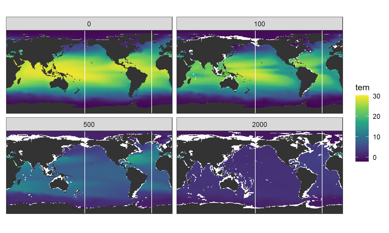
3.2.2 Sections
section_climatology_Atl(WOA_tem_tibble, "tem")
section_climatology_Pac(WOA_tem_tibble, "tem")
3.3 Salinity plots
3.3.1 Surface map
map_climatology(WOA_sal_tibble, "sal")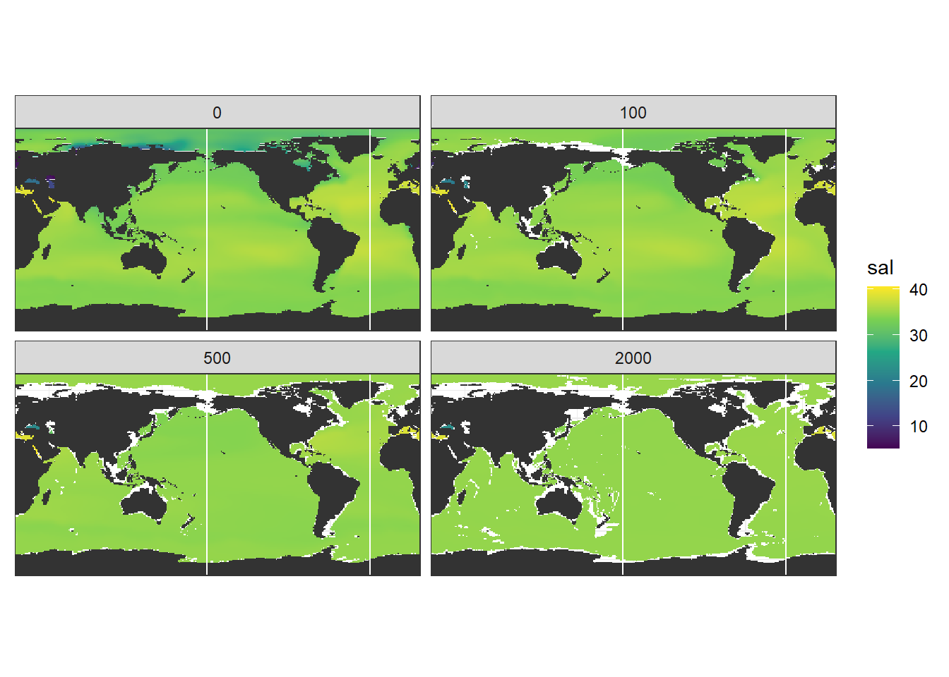
3.3.2 Sections
section_climatology_Atl(WOA_sal_tibble, "sal")
section_climatology_Pac(WOA_sal_tibble, "sal")
3.4 Write file
WOA18_predictors <- full_join(WOA_sal_tibble, WOA_tem_tibble)

WOA18_predictors %>%
  write_csv(here::here("data/World_Ocean_Atlas_2018/_summarized_files",
                       "WOA18_predictors.csv"))

rm(WOA18_predictors, WOA_sal, WOA_sal_tibble, WOA_tem, WOA_tem_tibble)
4 WOA13 from D. Clement
Dominic Clement provided a netcdf file with the basin mask and neutral densities used in Clement and Gruber (2018), both derived from the World Ocean Atlas 2013.
4.1 Read ncdfs
# temperature

nd_mask <- tidync(here::here("data/dclement",
                          "nd_mask.nc"))
nd_mask_tibble <- nd_mask %>% hyper_tibble()

nd_mask_tibble <- nd_mask_tibble %>%
  mutate(gamma = if_else(gamma == -999, NaN, gamma))
4.2 Plots
depth_surface_selection <- c(0)
Atl_lon <- 335.5
Pac_lon <- 190.5
Below, following subsets of the climatologies are plotted:
- Basin mask at 0m
- Meridional sections of neutral density at longitudes:
- Atlantic: 335.5
- Pacific: 190.5
Section locations are indicated as white lines in the basin map.
4.3 Basin map
nd_mask_tibble %>%
  filter(depth == 0) %>%
  ggplot(aes(longitude, latitude, fill = as.factor(mask))) +
  geom_raster() +
  geom_vline(xintercept = c(Atl_lon, Pac_lon), col = "white") +
  coord_quickmap(expand = 0) +
  scale_fill_brewer(palette = "Set1",
                    name = "basin mask") +
  theme(legend.position = "top")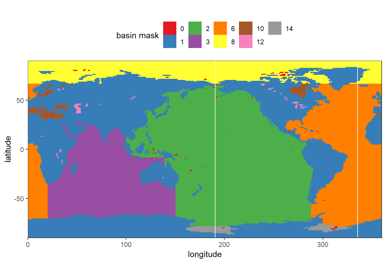
4.4 Neutral density sections
4.4.1 Atlantic
nd_mask_tibble %>%
  filter(longitude == Atl_lon) %>%
  ggplot(aes(latitude, depth, z = gamma)) +
  geom_contour_filled() +
  scale_y_reverse() +
  coord_cartesian(expand = 0) +
  theme(legend.position = "top")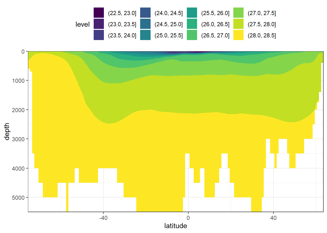
4.4.2 Pacific
nd_mask_tibble %>%
  filter(longitude == Pac_lon) %>%
  ggplot(aes(latitude, depth, z = gamma)) +
  geom_contour_filled() +
  scale_y_reverse() +
  coord_cartesian(expand = 0) +
  theme(legend.position = "top")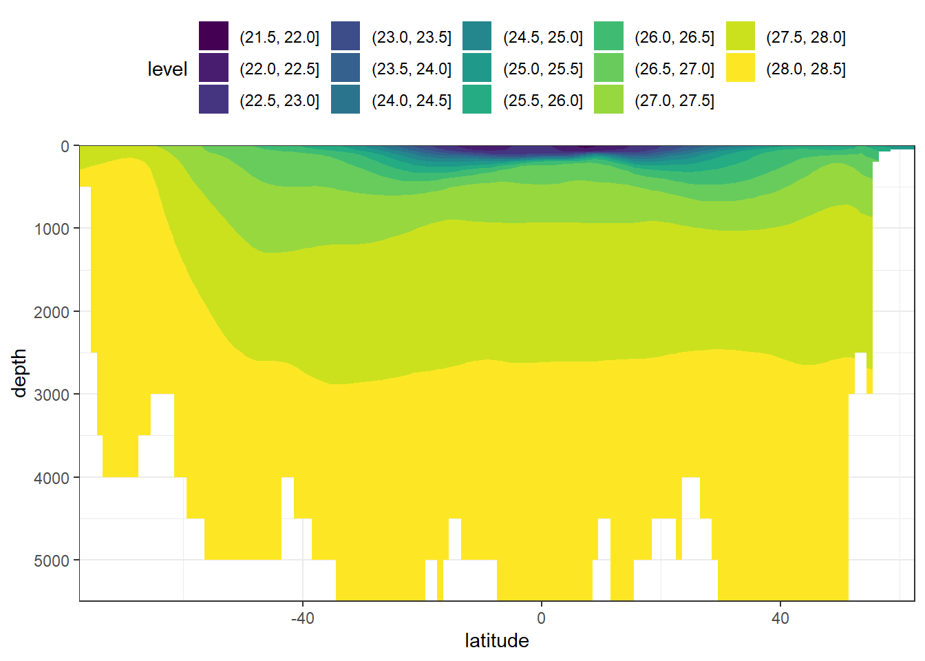
4.5 Write file
nd_mask_tibble %>%
  write_csv(here::here("data/World_Ocean_Atlas_2018/_summarized_files",
                       "WOA13_mask_gamma.csv"))

rm(nd_mask, nd_mask_tibble, Atl_lon, Pac_lon, depth_surface_selection)
5 Open tasks
- apply basin mask to WOA18 data
- add Indian ocean section plot
6 Questions
- Which version of the WOA to be used
- Fields (currently: objectively analyzed mean)
- Decades (currently: oall decades)
- Grid (currently: o1 deg resolution)
- How to merge with GLODAP climatology (currently interpolated to GLODAP depth)
sessionInfo()R version 4.0.2 (2020-06-22)
Platform: x86_64-w64-mingw32/x64 (64-bit)
Running under: Windows 10 x64 (build 18363)
Matrix products: default
locale:
[1] LC_COLLATE=English_Germany.1252 LC_CTYPE=English_Germany.1252
[3] LC_MONETARY=English_Germany.1252 LC_NUMERIC=C
[5] LC_TIME=English_Germany.1252
attached base packages:
[1] stats graphics grDevices utils datasets methods base
other attached packages:
[1] stars_0.4-3 sf_0.9-5 abind_1.4-5 tidync_0.2.4
[5] lubridate_1.7.9 forcats_0.5.0 stringr_1.4.0 dplyr_1.0.0
[9] purrr_0.3.4 readr_1.3.1 tidyr_1.1.0 tibble_3.0.3
[13] ggplot2_3.3.2 tidyverse_1.3.0 workflowr_1.6.2
loaded via a namespace (and not attached):
[1] httr_1.4.2 viridisLite_0.3.0 jsonlite_1.7.0 here_0.1
[5] modelr_0.1.8 assertthat_0.2.1 blob_1.2.1 cellranger_1.1.0
[9] yaml_2.2.1 pillar_1.4.6 backports_1.1.8 glue_1.4.1
[13] digest_0.6.25 RColorBrewer_1.1-2 promises_1.1.1 rvest_0.3.6
[17] colorspace_1.4-1 htmltools_0.5.0 httpuv_1.5.4 pkgconfig_2.0.3
[21] broom_0.7.0 haven_2.3.1 scales_1.1.1 whisker_0.4
[25] later_1.1.0.1 git2r_0.27.1 generics_0.0.2 farver_2.0.3
[29] ellipsis_0.3.1 withr_2.2.0 cli_2.0.2 magrittr_1.5
[33] crayon_1.3.4 readxl_1.3.1 evaluate_0.14 fs_1.4.2
[37] ncdf4_1.17 fansi_0.4.1 xml2_1.3.2 lwgeom_0.2-5
[41] class_7.3-17 tools_4.0.2 hms_0.5.3 lifecycle_0.2.0
[45] munsell_0.5.0 reprex_0.3.0 isoband_0.2.2 compiler_4.0.2
[49] e1071_1.7-3 RNetCDF_2.3-1 rlang_0.4.7 classInt_0.4-3
[53] units_0.6-7 grid_4.0.2 rstudioapi_0.11 labeling_0.3
[57] rmarkdown_2.3 gtable_0.3.0 DBI_1.1.0 R6_2.4.1
[61] ncmeta_0.2.5 knitr_1.29 rprojroot_1.3-2 KernSmooth_2.23-17
[65] stringi_1.4.6 parallel_4.0.2 Rcpp_1.0.5 vctrs_0.3.2
[69] dbplyr_1.4.4 tidyselect_1.1.0 xfun_0.16