Last updated: 2020-11-03

Checks: 7 0

Knit directory: Cant_eMLR/

This reproducible R Markdown analysis was created with workflowr (version 1.6.2). The Checks tab describes the reproducibility checks that were applied when the results were created. The Past versions tab lists the development history.

R Markdown file: up-to-date

Great! Since the R Markdown file has been committed to the Git repository, you know the exact version of the code that produced these results.

Environment: empty

Great job! The global environment was empty. Objects defined in the global environment can affect the analysis in your R Markdown file in unknown ways. For reproduciblity it’s best to always run the code in an empty environment.

Seed: set.seed(20200707)

The command set.seed(20200707) was run prior to running the code in the R Markdown file. Setting a seed ensures that any results that rely on randomness, e.g. subsampling or permutations, are reproducible.

Session information: recorded

Great job! Recording the operating system, R version, and package versions is critical for reproducibility.

Cache: none

Nice! There were no cached chunks for this analysis, so you can be confident that you successfully produced the results during this run.

File paths: relative

Great job! Using relative paths to the files within your workflowr project makes it easier to run your code on other machines.

Repository version: bfa7a21

Great! You are using Git for version control. Tracking code development and connecting the code version to the results is critical for reproducibility.

The results in this page were generated with repository version bfa7a21. See the Past versions tab to see a history of the changes made to the R Markdown and HTML files.

Note that you need to be careful to ensure that all relevant files for the analysis have been committed to Git prior to generating the results (you can use wflow_publish or wflow_git_commit). workflowr only checks the R Markdown file, but you know if there are other scripts or data files that it depends on. Below is the status of the Git repository when the results were generated:


Ignored files:
    Ignored:    .Rproj.user/
    Ignored:    data/GLODAPv1_1/
    Ignored:    data/GLODAPv2_2016b_MappedClimatologies/
    Ignored:    data/GLODAPv2_2020/
    Ignored:    data/Gruber_2019/
    Ignored:    data/WOCE/
    Ignored:    data/World_Ocean_Atlas_2013_Clement/
    Ignored:    data/World_Ocean_Atlas_2018/
    Ignored:    data/eMLR/
    Ignored:    data/mapping/
    Ignored:    data/pCO2_atmosphere/
    Ignored:    dump/

Untracked files:
    Untracked:  code/globe_3d.R

Unstaged changes:
    Modified:   analysis/_site.yml
    Modified:   code/Workflowr_project_managment.R

Note that any generated files, e.g. HTML, png, CSS, etc., are not included in this status report because it is ok for generated content to have uncommitted changes.

These are the previous versions of the repository in which changes were made to the R Markdown (analysis/analysis_this_study.Rmd) and HTML (docs/analysis_this_study.html) files. If you’ve configured a remote Git repository (see ?wflow_git_remote), click on the hyperlinks in the table below to view the files as they were in that past version.

File	Version	Author	Date	Message
html	411a35b	jens-daniel-mueller	2020-10-02	Build site.
html	0d38979	jens-daniel-mueller	2020-10-01	Build site.
html	9f28fef	jens-daniel-mueller	2020-10-01	Build site.
Rmd	812e71b	jens-daniel-mueller	2020-10-01	seperate globe rmd
html	35649f2	jens-daniel-mueller	2020-09-30	Build site.
Rmd	5418fb9	jens-daniel-mueller	2020-09-30	added globes for both eras
html	80e9b77	jens-daniel-mueller	2020-09-30	Build site.
Rmd	1794dc7	jens-daniel-mueller	2020-09-30	added 3d globe vis
html	4578cfa	jens-daniel-mueller	2020-09-19	Build site.
html	b1d66e7	jens-daniel-mueller	2020-09-19	Build site.
Rmd	eb34789	jens-daniel-mueller	2020-09-19	gamma slab on depth levels plotted
html	d285219	jens-daniel-mueller	2020-09-18	Build site.
Rmd	60efbf7	jens-daniel-mueller	2020-09-18	revised panel order
html	d59f716	jens-daniel-mueller	2020-09-18	Build site.
Rmd	27809b8	jens-daniel-mueller	2020-09-18	restricted tco2 f flag to 2
html	9bbf9ee	jens-daniel-mueller	2020-09-18	Build site.
Rmd	a678e01	jens-daniel-mueller	2020-09-18	resolved cant budget by basin
html	20b9238	jens-daniel-mueller	2020-09-18	Build site.
Rmd	7abc2dd	jens-daniel-mueller	2020-09-18	formatted table
html	3ef6906	jens-daniel-mueller	2020-09-18	Build site.
Rmd	5bfaf2a	jens-daniel-mueller	2020-09-18	included cant budgets
html	0d94630	jens-daniel-mueller	2020-09-18	Build site.
Rmd	bf31773	jens-daniel-mueller	2020-09-18	rearranged plots
html	e120224	jens-daniel-mueller	2020-09-18	Build site.
Rmd	39fe9d0	jens-daniel-mueller	2020-09-18	rearranged plots
html	96e3f0a	jens-daniel-mueller	2020-09-18	Build site.
Rmd	6ebc455	jens-daniel-mueller	2020-09-18	rearranged and revised plots
html	8ddeeac	jens-daniel-mueller	2020-09-18	Build site.
Rmd	3fe7f52	jens-daniel-mueller	2020-09-18	rearranged plots
html	88e474a	jens-daniel-mueller	2020-09-18	Build site.
Rmd	cf9b9d7	jens-daniel-mueller	2020-09-18	zonal mean section gruber color scale
html	21668f6	jens-daniel-mueller	2020-09-18	Build site.
Rmd	3838220	jens-daniel-mueller	2020-09-18	zonal mean section gruber color scale
html	9b35dd0	jens-daniel-mueller	2020-09-18	Build site.
Rmd	4b8cb4e	jens-daniel-mueller	2020-09-18	zonal mean section gruber color scale
html	b68196d	jens-daniel-mueller	2020-09-18	Build site.
Rmd	7c0354d	jens-daniel-mueller	2020-09-18	mean sections with gruber color scale
html	59e9bcd	jens-daniel-mueller	2020-09-18	Build site.
Rmd	df65c0a	jens-daniel-mueller	2020-09-18	applied Gruber 2019 color scale
html	f5a20ac	jens-daniel-mueller	2020-09-17	Build site.
Rmd	10c1a10	jens-daniel-mueller	2020-09-17	added Cant along slab
html	cf64460	jens-daniel-mueller	2020-09-17	Build site.
html	9d9a553	jens-daniel-mueller	2020-09-17	Build site.
Rmd	a7e8ba5	jens-daniel-mueller	2020-09-17	rebuild after complete collapse averaging
html	abc176a	jens-daniel-mueller	2020-09-17	Build site.
Rmd	ca05234	jens-daniel-mueller	2020-09-17	collapse averaging for all big data sets
html	1ea7231	jens-daniel-mueller	2020-09-17	Build site.
html	d43d9e2	jens-daniel-mueller	2020-09-16	Build site.
html	605e13b	jens-daniel-mueller	2020-09-16	Build site.
html	1f3319a	jens-daniel-mueller	2020-09-16	Build site.
html	19d4d56	jens-daniel-mueller	2020-09-16	Build site.
html	55f86a6	jens-daniel-mueller	2020-09-15	Build site.
Rmd	b9d37ab	jens-daniel-mueller	2020-09-15	observations per density slab included
html	2cd847c	jens-daniel-mueller	2020-09-14	Build site.
Rmd	1a13af4	jens-daniel-mueller	2020-09-14	replace all model sections plots chunk
html	da91d98	jens-daniel-mueller	2020-09-10	Build site.
html	454e665	jens-daniel-mueller	2020-09-10	Build site.
Rmd	c7ae6ab	jens-daniel-mueller	2020-09-10	updated plots
html	1124ca5	jens-daniel-mueller	2020-09-10	Build site.
Rmd	27c5ab1	jens-daniel-mueller	2020-09-10	updated plots
html	382ffba	jens-daniel-mueller	2020-09-10	Build site.
Rmd	d37bb48	jens-daniel-mueller	2020-09-10	updated plots
html	a34a239	jens-daniel-mueller	2020-09-10	Build site.
html	2458576	jens-daniel-mueller	2020-09-09	Build site.
html	e60e13c	jens-daniel-mueller	2020-09-09	Build site.
Rmd	7040b80	jens-daniel-mueller	2020-09-09	remove basin_AIP not covered by mapping
html	c3ffdfd	jens-daniel-mueller	2020-09-08	Build site.
Rmd	04ee730	jens-daniel-mueller	2020-09-08	rebuild after revision
html	793f996	jens-daniel-mueller	2020-09-07	Build site.
Rmd	2d1300a	jens-daniel-mueller	2020-09-07	added all predictor plots
html	148db18	jens-daniel-mueller	2020-09-07	Build site.
Rmd	0bea059	jens-daniel-mueller	2020-09-07	plotted predictor contribution zonal mean
html	a50f053	jens-daniel-mueller	2020-09-07	Build site.
html	da445a6	jens-daniel-mueller	2020-09-04	Build site.
Rmd	6a302ca	jens-daniel-mueller	2020-09-04	rebuild after new data cleaning and mapping Cant to surface
html	fa11a74	jens-daniel-mueller	2020-09-02	Build site.
html	429aab3	jens-daniel-mueller	2020-09-01	Build site.
html	f4216dd	jens-daniel-mueller	2020-09-01	Build site.
html	13a76d5	jens-daniel-mueller	2020-08-28	Build site.
Rmd	2e6a4ca	jens-daniel-mueller	2020-08-28	XXX
html	1f05c5d	jens-daniel-mueller	2020-08-28	Build site.
Rmd	5ad6a52	jens-daniel-mueller	2020-08-28	added gamma maps and switched to depth levels 150, 500, 1000, 2000
html	27404de	jens-daniel-mueller	2020-08-27	Build site.
html	cfdb312	jens-daniel-mueller	2020-08-27	Build site.
Rmd	a4d0f62	jens-daniel-mueller	2020-08-27	plotting with functions
html	b6d0e6a	jens-daniel-mueller	2020-08-27	Build site.
html	fc4f889	jens-daniel-mueller	2020-08-26	Build site.
Rmd	a3e427c	jens-daniel-mueller	2020-08-26	Cant vs regional SD added
html	f37f6b6	jens-daniel-mueller	2020-08-26	Build site.
Rmd	ce109c0	jens-daniel-mueller	2020-08-26	Cant vs SD plotted
html	e951135	jens-daniel-mueller	2020-08-26	Build site.
Rmd	7f3a671	jens-daniel-mueller	2020-08-26	Cant vs SD plotted
html	f40e48b	jens-daniel-mueller	2020-08-26	Build site.
Rmd	b577ec6	jens-daniel-mueller	2020-08-26	Analysis split in this and previous studies

library(tidyverse)
library(patchwork)
library(scico)
library(scales)
library(metR)
library(marelac)
library(kableExtra)
library(threejs)

1 Data sources

Cant estimates from this study:

Mean and SD per grid cell (lat, lon, depth)
Zonal mean and SD (basin, lat, depth)
Inventories (lat, lon)

Cant_average <-
  read_csv(here::here("data/mapping/_summarized_files",
                         "Cant_average.csv"))

Cant_average_zonal <-
  read_csv(here::here("data/mapping/_summarized_files",
                         "Cant_average_zonal.csv"))

Cant_predictor_average_zonal <-
  read_csv(here::here("data/mapping/_summarized_files",
                         "Cant_predictor_average_zonal.csv"))

Cant_inv <-
  read_csv(here::here("data/mapping/_summarized_files",
                         "Cant_inv.csv"))

C* estimates from this study:

Mean and SD per grid cell (lat, lon, depth)
Zonal mean and SD (basin, lat, depth)

Cstar_average <-
  read_csv(here::here("data/mapping/_summarized_files",
                         "Cstar_average.csv"))

Cstar_average_zonal <-
  read_csv(here::here("data/mapping/_summarized_files",
                         "Cstar_average_zonal.csv"))

Cleaned GLODAPv2_2020 file as used in this study

GLODAP <-
  read_csv(
    here::here(
      "data/GLODAPv2_2020/_summarized_data_files",
      "GLODAP_MLR_fitting_ready.csv"
    )
  )

2 Color scale

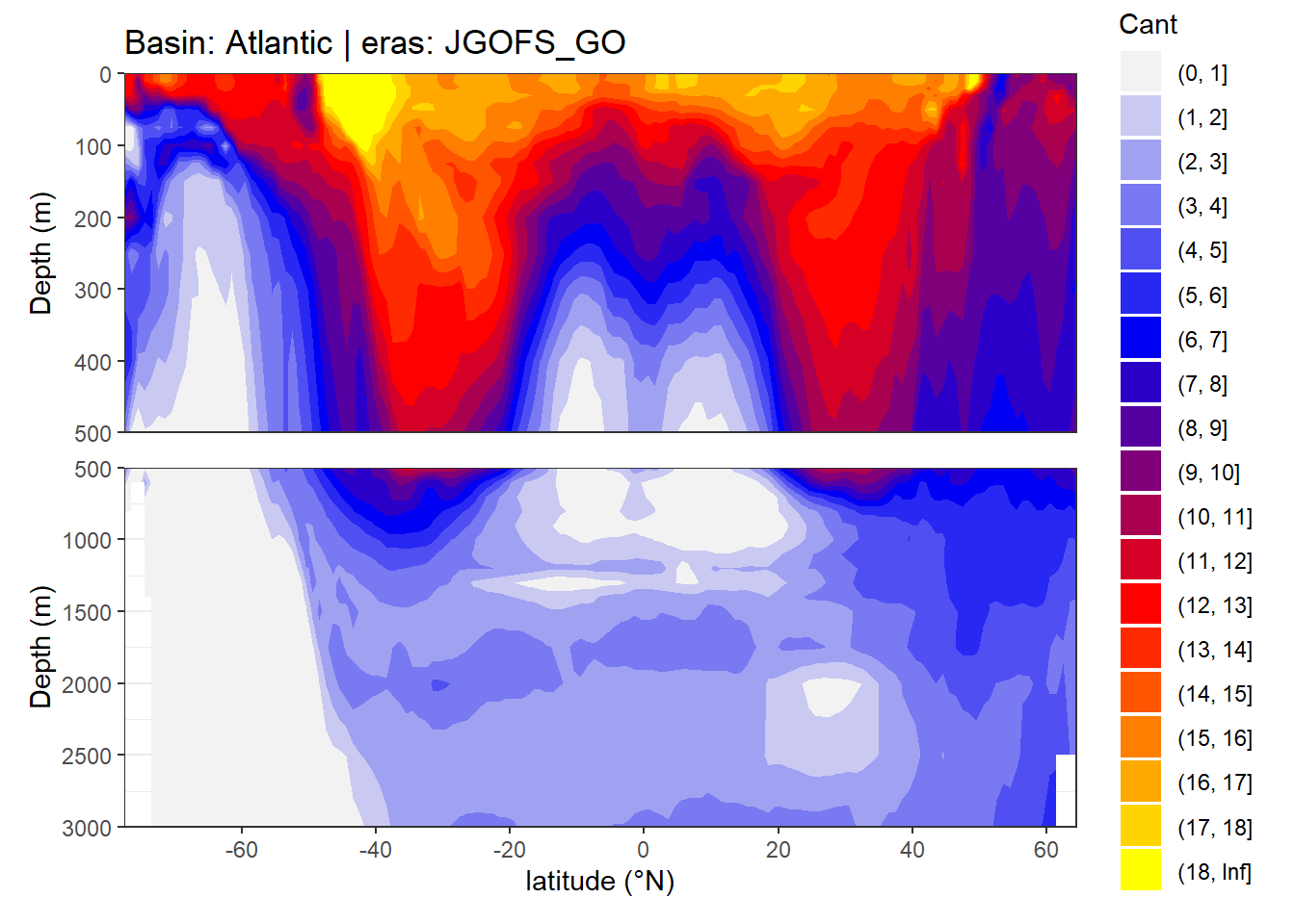
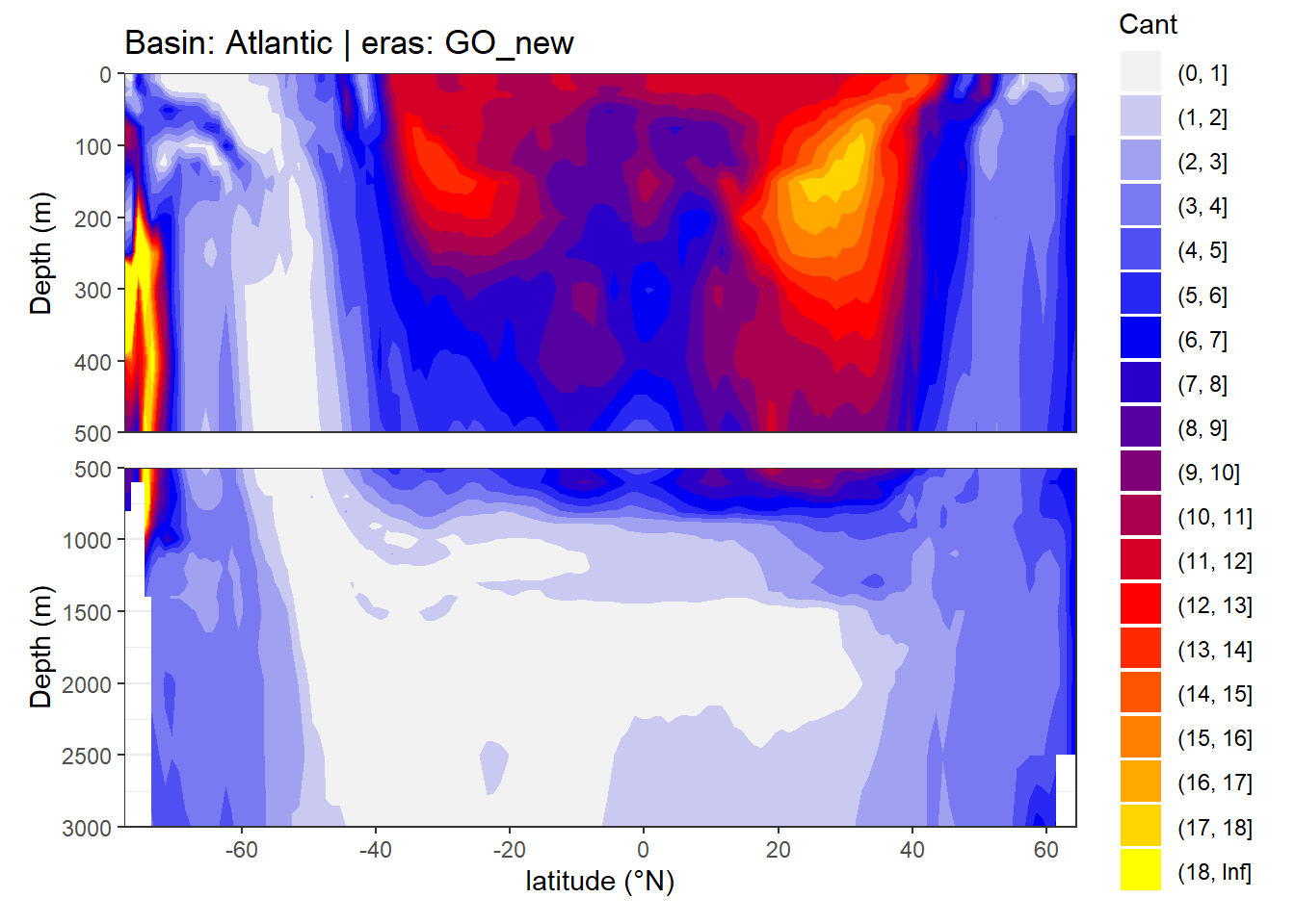
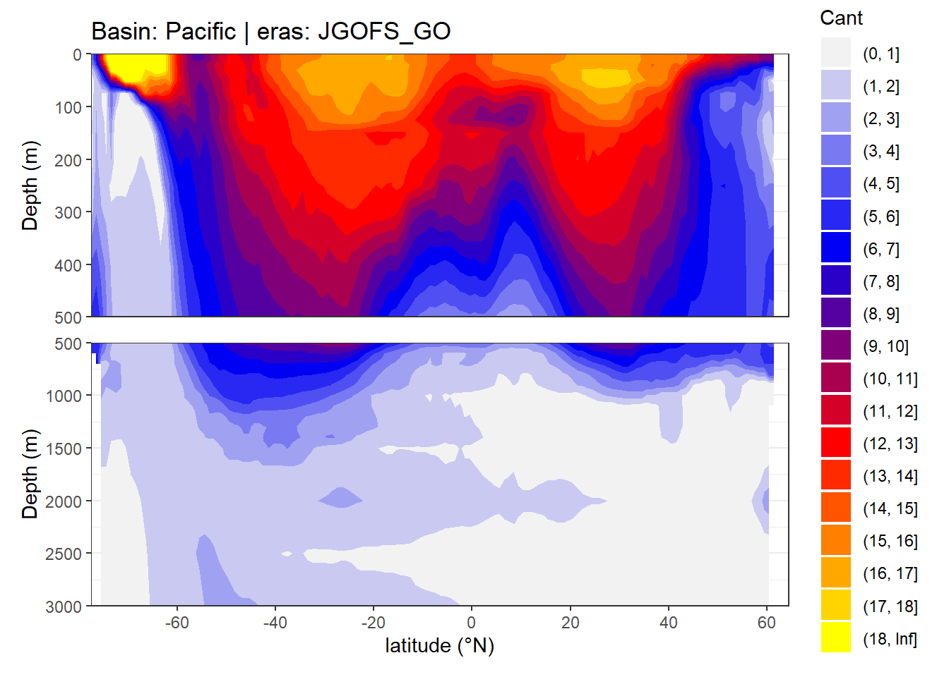
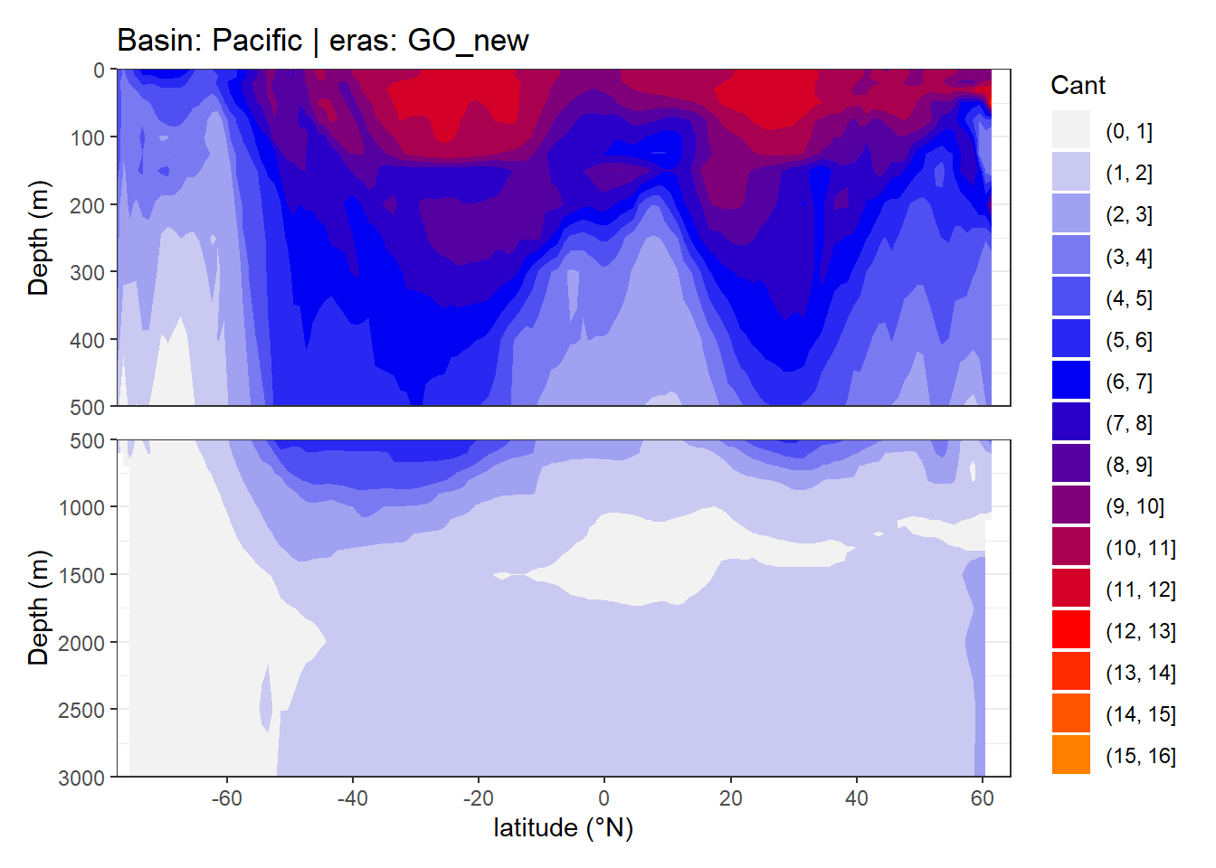
For ease of comparison with Gruber et al (2019) we adapt their color scale, including the ranges and breaks applied in various types of visualizations.

rgb2hex <- function(r, g, b)
  rgb(r, g, b, maxColorValue = 100)

cols = c(rgb2hex(95, 95, 95),
         rgb2hex(0, 0, 95),
         rgb2hex(100, 0, 0),
         rgb2hex(100, 100, 0))

Gruber_rainbow <- colorRampPalette(cols)

rm(rgb2hex, cols)

3 Cant budgets

Global Cant inventories were estimated in Pg-C. Please note that here we only added positive Cant values in the upper 3000m and do not apply additional corrections for areas not covered.

Cant_inv <- left_join(Cant_inv, basinmask_AIP) 

Cant_inv_budget <- Cant_inv %>% 
  mutate(surface_area = earth_surf(lat, lon),
         cant_inv_grid = cant_inv*surface_area) %>% 
  group_by(eras, basin_AIP) %>% 
  summarise(cant_total = sum(cant_inv_grid)*12*1e-15,
            cant_total = round(cant_total,1)) %>% 
  ungroup() %>% 
  arrange(desc(eras)) %>% 
  pivot_wider(values_from = cant_total, names_from = basin_AIP) %>% 
  mutate(total = Atlantic + Indian + Pacific)

Cant_inv_budget %>% 
  kableExtra::kable() %>% 
  add_header_above() %>%
  kable_styling(full_width = FALSE)

eras	Atlantic	Indian	Pacific	total
JGOFS_GO	9.9	10.1	17.5	37.5
GO_new	6.9	3.9	13.6	24.4

rm(Cant_inv_budget)

4 Cant - positive

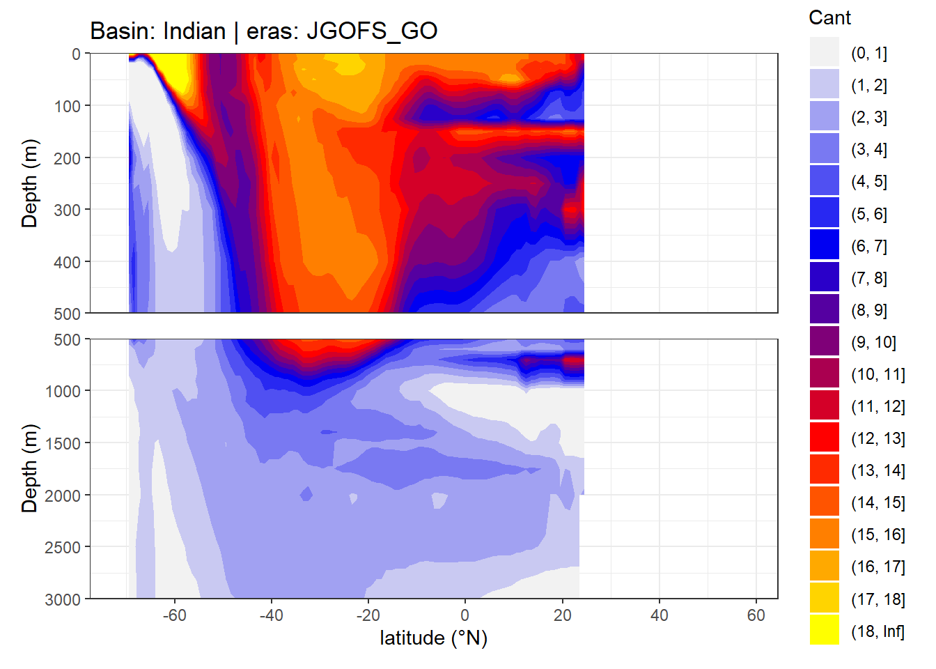
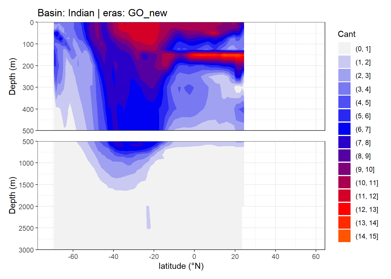
In a first series of plots we explore the distribution of Cant, taking only positive estimates into account (positive here refers to the mean Cant estimate across 10 eMLR model predictions available for each grid cell). Negative values were set to zero before calculating mean sections and inventories.

4.1 Zonal mean sections

Cant_average_zonal <- Cant_average_zonal %>% 
  mutate(eras = factor(eras, c("JGOFS_GO", "GO_new")))

breaks <- c(seq(0,18,1),Inf)
breaks_n <- length(breaks) - 1

Cant_average_zonal <- Cant_average_zonal %>% 
  mutate(Cant_pos_mean_int = cut(Cant_pos_mean, 
                                breaks,
                                right = FALSE))


zonal_section <- function(df, i_basin_AIP, i_eras, var) {
  
  name_var <- var
  var <- sym(var)
  
  lat_max <- max(df$lat)
  lat_min <- min(df$lat)
  
  df_sub <- df %>% 
    filter(eras == i_eras,
           basin_AIP == i_basin_AIP)
  
  surface <- df_sub %>%
    ggplot(aes(lat, depth, z = !!var)) +
    geom_contour_filled(breaks = breaks) +
    scale_fill_manual(values = Gruber_rainbow(breaks_n),
                      name = "Cant") +
    coord_cartesian(expand = 0,
                    ylim = c(500, 0),
                    xlim = c(lat_min, lat_max)) +
    scale_y_reverse() +
    scale_x_continuous(breaks = seq(-100,100,20)) +
    theme(
      axis.title.x = element_blank(),
      axis.text.x = element_blank(),
      axis.ticks.x = element_blank()
    ) +
    labs(y = "Depth (m)",
         title = paste("Basin:", i_basin_AIP, "| eras:", i_eras))
  
  deep <- df_sub %>%
    ggplot(aes(lat, depth, z = !!var)) +
    geom_contour_filled(breaks = breaks) +
    scale_fill_manual(values = Gruber_rainbow(breaks_n),
                      name = "Cant") +
    scale_y_reverse() +
    scale_x_continuous(breaks = seq(-100,100,20)) +
    coord_cartesian(expand = 0,
                    ylim = c(3000, 500),
                    xlim = c(lat_min, lat_max)) +
    labs(x = "latitude (°N)", y = "Depth (m)")
  
  surface / deep +
    plot_layout(guides = "collect")
  
}


for (i_basin_AIP in unique(Cant_average_zonal$basin_AIP)) {
  for (i_eras in rev(unique(Cant_average_zonal$eras))) {
    
    print(zonal_section(Cant_average_zonal,
                        i_basin_AIP = i_basin_AIP,
                        i_eras = i_eras,
                        "Cant_pos_mean"))
    
  }
  
}

rm(breaks, breaks_n)

4.2 Isoneutral slab distribution

Mean of positive Cant within each horizontal grid cell (lon x lat) per isoneutral slab.

Please note that:

density slabs covering values >28.1 occur by definition only either in the Atlantic or Indo-Pacific basin
gaps in the maps represent areas where (thin) density layers fit between discrete depth levels used for mapping

Cant_gamma_maps <- Cant_average %>% 
  group_by(lat, lon, gamma_slab, eras) %>% 
  summarise(Cant_pos = mean(Cant_pos, na.rm = TRUE)) %>% 
  ungroup()


breaks <- c(seq(0,16,2),Inf)
breaks_n <- length(breaks) - 1

Cant_gamma_maps <- Cant_gamma_maps %>% 
  mutate(Cant_pos_int = cut(Cant_pos, 
                                breaks,
                                right = FALSE)) %>% 
  mutate(eras = factor(eras, c("JGOFS_GO", "GO_new")))


ggplot() +
  geom_raster(data = landmask,
              aes(lon, lat),
              fill = "grey30") +
  geom_raster(data = Cant_gamma_maps,
              aes(lon, lat, fill = Cant_pos_int)) +
  scale_fill_manual(values = Gruber_rainbow(breaks_n)) +
  facet_grid(gamma_slab ~ eras) +
  coord_quickmap(expand = 0) +
  theme(axis.title = element_blank(),
        axis.ticks = element_blank(),
        axis.text = element_blank(),
        legend.position = "top")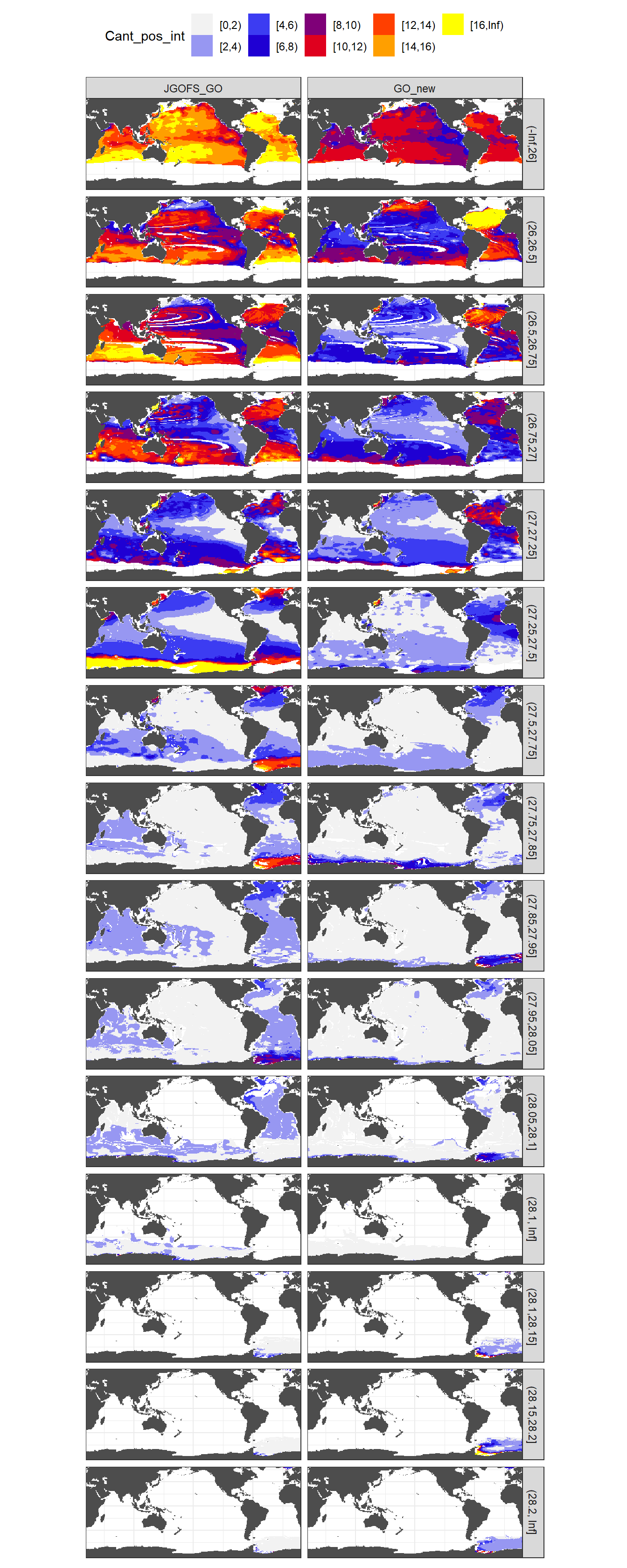

rm(Cant_gamma_maps, breaks, breaks_n)

4.3 Inventory map

Column inventory of positive Cant between the surface and 3000m water depth per horizontal grid cell (lat x lon).

breaks <- c(seq(0,16,2),Inf)
breaks_n <- length(breaks) - 1

Cant_inv <- Cant_inv %>% 
  mutate(cant_inv_pos_int = cut(cant_inv_pos, 
                                breaks,
                                right = FALSE)) %>% 
  mutate(eras = factor(eras, c("JGOFS_GO", "GO_new")))

Cant_inv %>%
  ggplot() +
  geom_raster(data = landmask,
              aes(lon, lat), fill = "grey30") +
  geom_raster(aes(lon, lat, fill = cant_inv_pos_int)) +
  coord_quickmap(expand = 0) +
  scale_fill_manual(values = Gruber_rainbow(breaks_n)) +
  # scale_fill_scico_d(palette = "batlow", direction = -1) +
  facet_wrap( ~ eras, ncol = 1) +
  theme(axis.title = element_blank())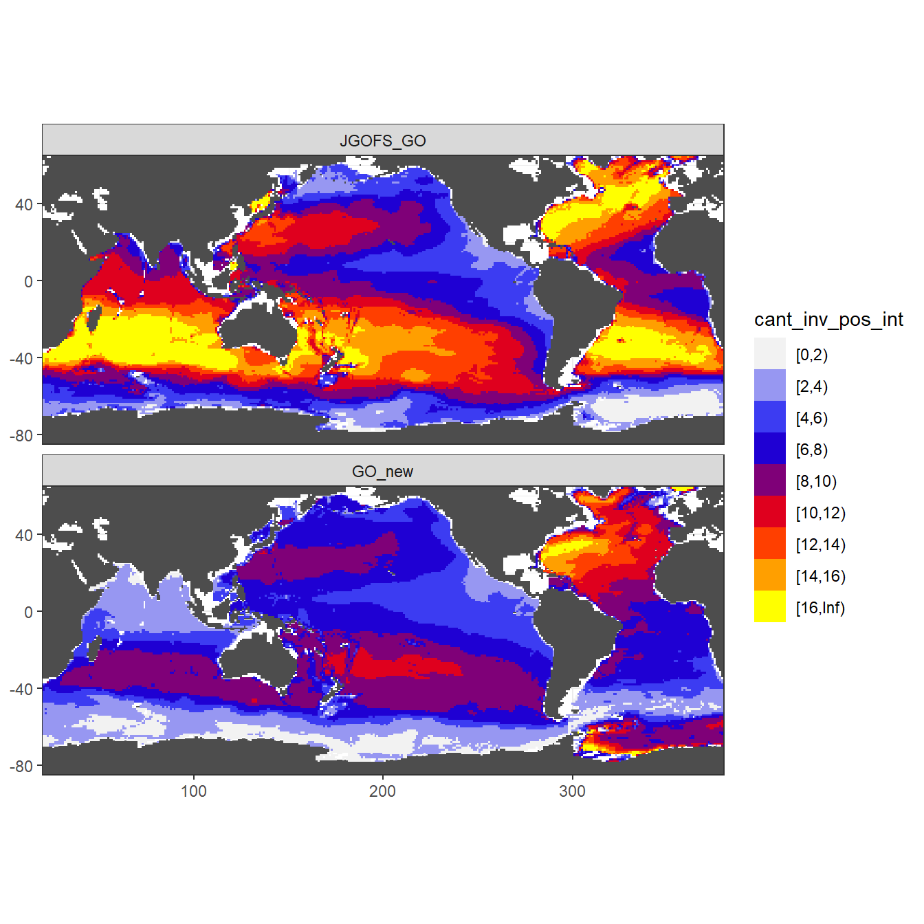

4.4 Global section

4.4.1 JGOFS_GO

section_global(Cant_average %>% filter(eras == "JGOFS_GO"),
                    "Cant_pos")

4.4.2 GO_new

section_global(Cant_average %>% filter(eras == "GO_new"),
                    "Cant_pos")

5 Cant - all

In a second series of plots we explore the distribution of Cant, taking positive and negative estimates into account.

5.1 Zonal mean sections

section_zonal_average_divergent(Cant_average_zonal,
                                "Cant_mean",
                                "gamma_mean")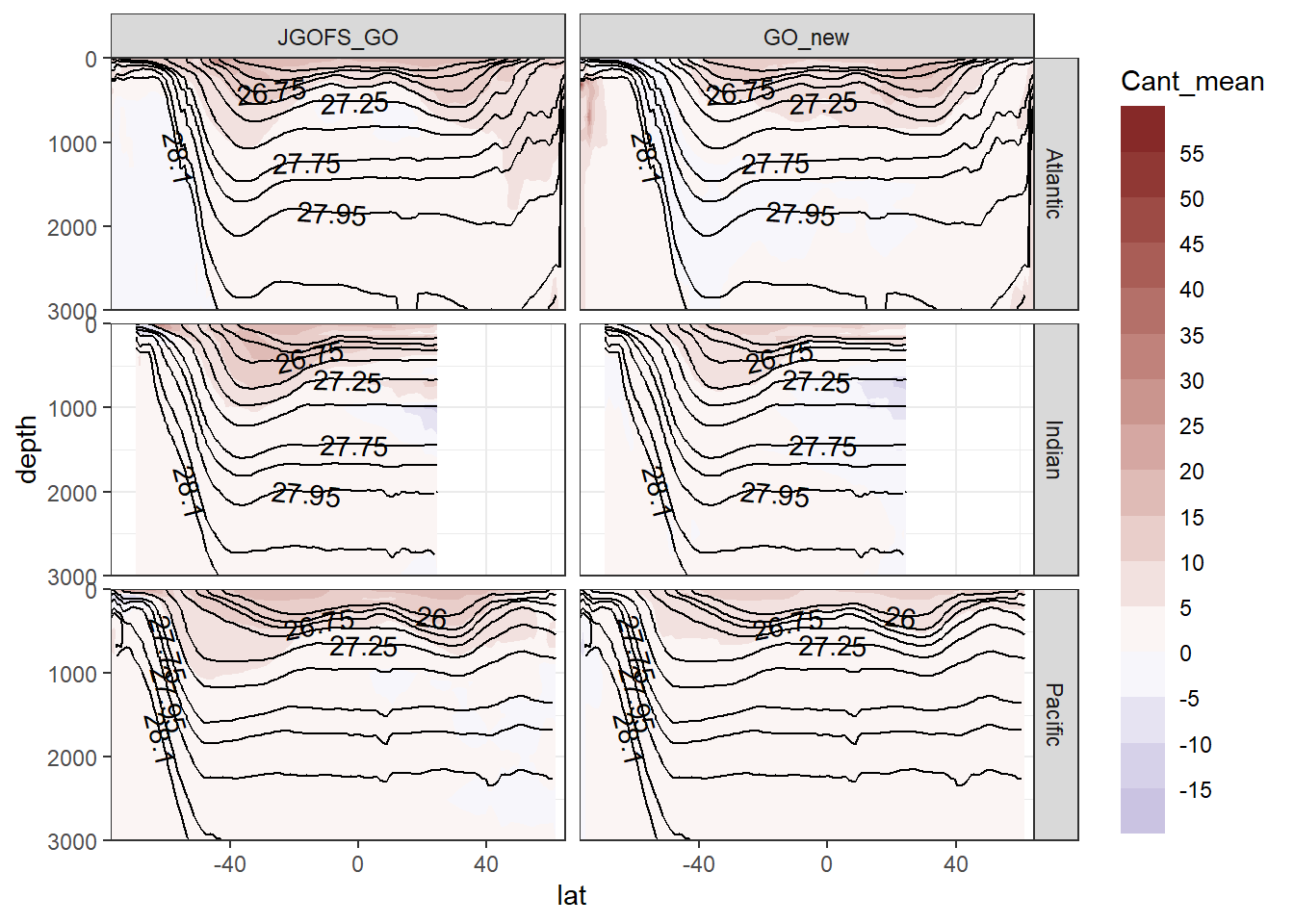

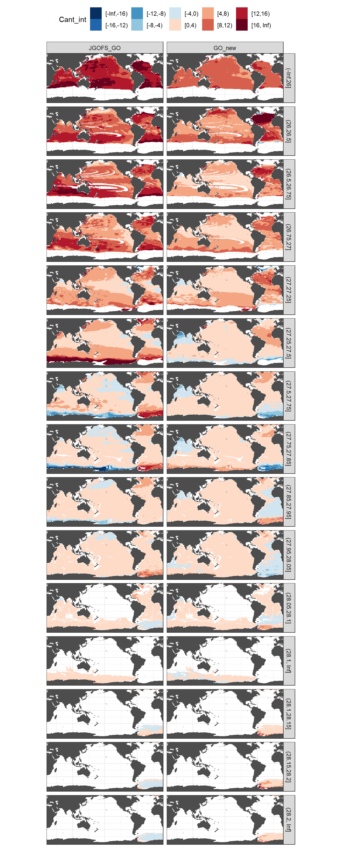
5.2 Isoneutral slab distribution

Mean of Cant within each horizontal grid cell (lon x lat) per isoneutral slab.

Please note that:

density slabs covering values >28.1 occur by definition only either in the Atlantic or Indo-Pacific basin
gaps in the maps represent areas where (thin) density layers fit between discrete depth levels used for mapping

Cant_gamma_maps <- Cant_average %>%
  group_by(lat, lon, gamma_slab, eras) %>%
  summarise(Cant = mean(Cant, na.rm = TRUE)) %>%
  ungroup()


breaks <- c(-Inf, seq(-16, 16, 4), Inf)
breaks_n <- length(breaks) - 1

Cant_gamma_maps <- Cant_gamma_maps %>%
  mutate(Cant_int = cut(Cant,
                        breaks,
                        right = FALSE)) %>% 
  mutate(eras = factor(eras, c("JGOFS_GO", "GO_new")))

ggplot() +
  geom_raster(data = landmask,
              aes(lon, lat),
              fill = "grey30") +
  geom_raster(data = Cant_gamma_maps,
              aes(lon, lat, fill = Cant_int)) +
  scale_fill_brewer(palette = "RdBu",
                    direction = -1) +
  facet_grid(gamma_slab ~ eras) +
  coord_quickmap(expand = 0) +
  theme(
    axis.title = element_blank(),
    axis.ticks = element_blank(),
    axis.text = element_blank(),
    legend.position = "top"
  )

rm(Cant_gamma_maps, breaks, breaks_n)

5.3 Inventory map

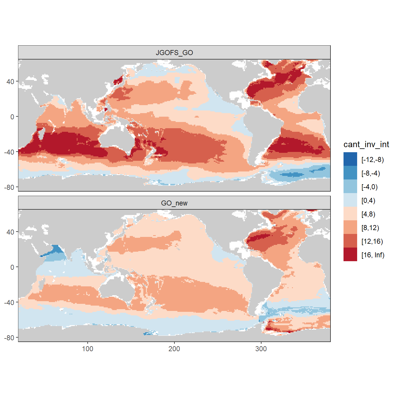
Column inventory of positive Cant between the surface and 3000m water depth per horizontal grid cell (lat x lon).

breaks <- c(-Inf, seq(-16,16,4),Inf)
breaks_n <- length(breaks) - 1

Cant_inv <- Cant_inv %>% 
  mutate(cant_inv_int = cut(cant_inv, 
                                breaks,
                                right = FALSE))
Cant_inv %>% 
  ggplot() +
    geom_raster(data = landmask,
                aes(lon, lat), fill = "grey80") +
    geom_raster(aes(lon, lat, fill = cant_inv_int)) +
    coord_quickmap(expand = 0) +
  scale_fill_brewer(palette = "RdBu",
                    direction = -1) +
  facet_wrap(~eras, ncol = 1) +
    theme(
      axis.title = element_blank()
    )

rm(breaks, breaks_n)

6 Cant - standard deviation

6.1 Across models

Standard deviation across Cant from all MLR models was calculate for each grid cell (XYZ). The zonal mean of this standard deviation should reflect the uncertainty associated to the predictor selection within each slab and era.

section_zonal_average_continous(Cant_average_zonal,
                                "Cant_sd_mean",
                                "gamma_mean")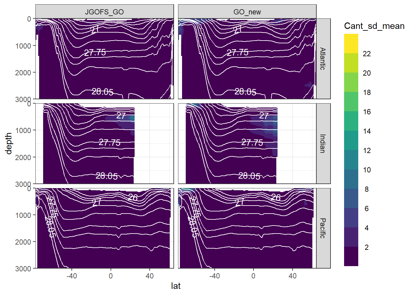

6.2 Across basins

Standard deviation of mean Cant values was calculate across all longitudes. This standard deviation should reflect the zonal variability of Cant within the basin and era.

section_zonal_average_continous(Cant_average_zonal,
                                "Cant_sd",
                                "gamma_mean")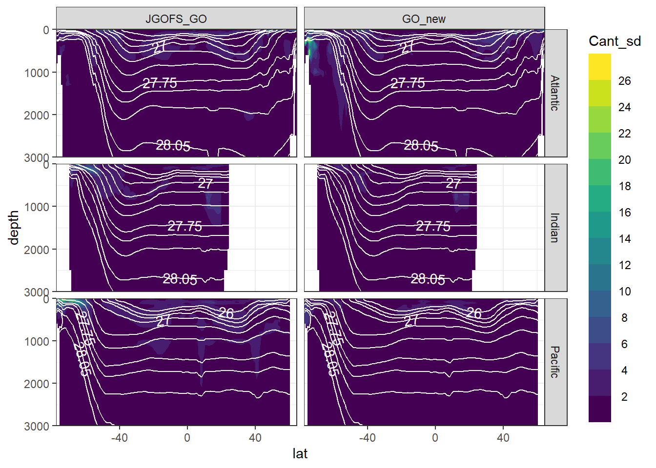

6.3 Correlation

6.3.1 Cant vs model SD

Cant_average <- Cant_average  %>% 
  mutate(eras = factor(eras, c("JGOFS_GO", "GO_new")))

Cant_average %>% 
  ggplot(aes(Cant, Cant_sd)) +
  geom_vline(xintercept = 0) +
  geom_hline(yintercept = 10) +
  geom_bin2d() +
  scale_fill_viridis_c(option = "magma",
                       direction = -1,
                       trans = "log10",
                       name = "log10(n)") +
  facet_grid(basin_AIP ~ eras)

Cant_average %>% 
  ggplot(aes(Cant, Cant_sd)) +
  geom_vline(xintercept = 0) +
  geom_hline(yintercept = 10) +
  geom_bin2d() +
  scale_fill_viridis_c(option = "magma",
                       direction = -1,
                       trans = "log10",
                       name = "log10(n)") +
  facet_grid(gamma_slab ~ basin_AIP)

6.3.2 Cant vs regional SD

Cant_average_zonal %>% 
  ggplot(aes(Cant_mean, Cant_sd)) +
  geom_vline(xintercept = 0) +
  geom_hline(yintercept = 10) +
  geom_bin2d() +
  scale_fill_viridis_c(option = "magma",
                       direction = -1,
                       trans = "log10",
                       name = "log10(n)") +
  facet_grid(basin_AIP ~ eras)

Cant_average_zonal %>% 
  ggplot(aes(Cant_mean, Cant_sd)) +
  geom_vline(xintercept = 0) +
  geom_hline(yintercept = 10) +
  geom_bin2d() +
  scale_fill_viridis_c(option = "magma",
                       direction = -1,
                       trans = "log10",
                       name = "log10(n)") +
  facet_grid(gamma_slab ~ basin_AIP)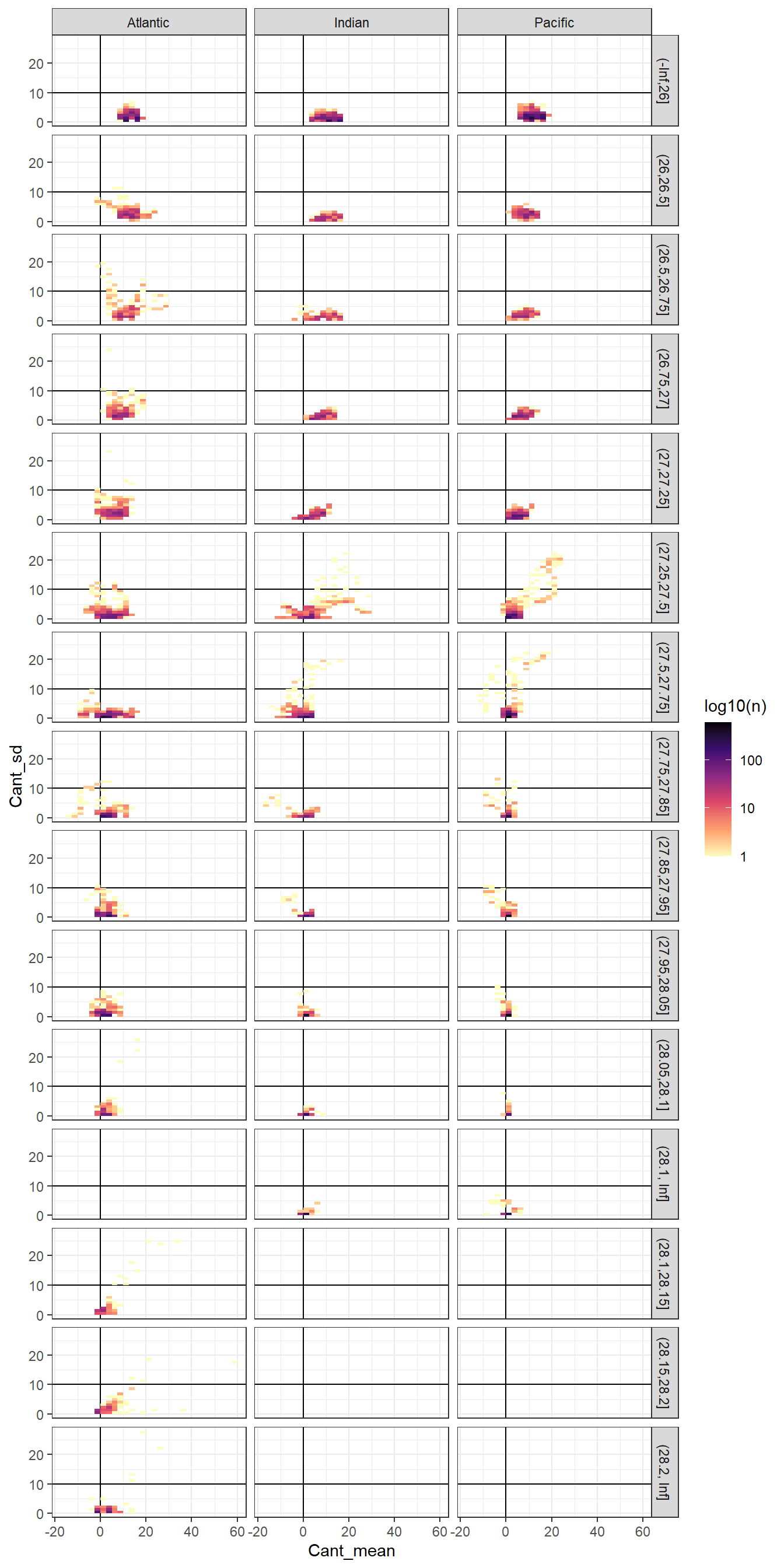

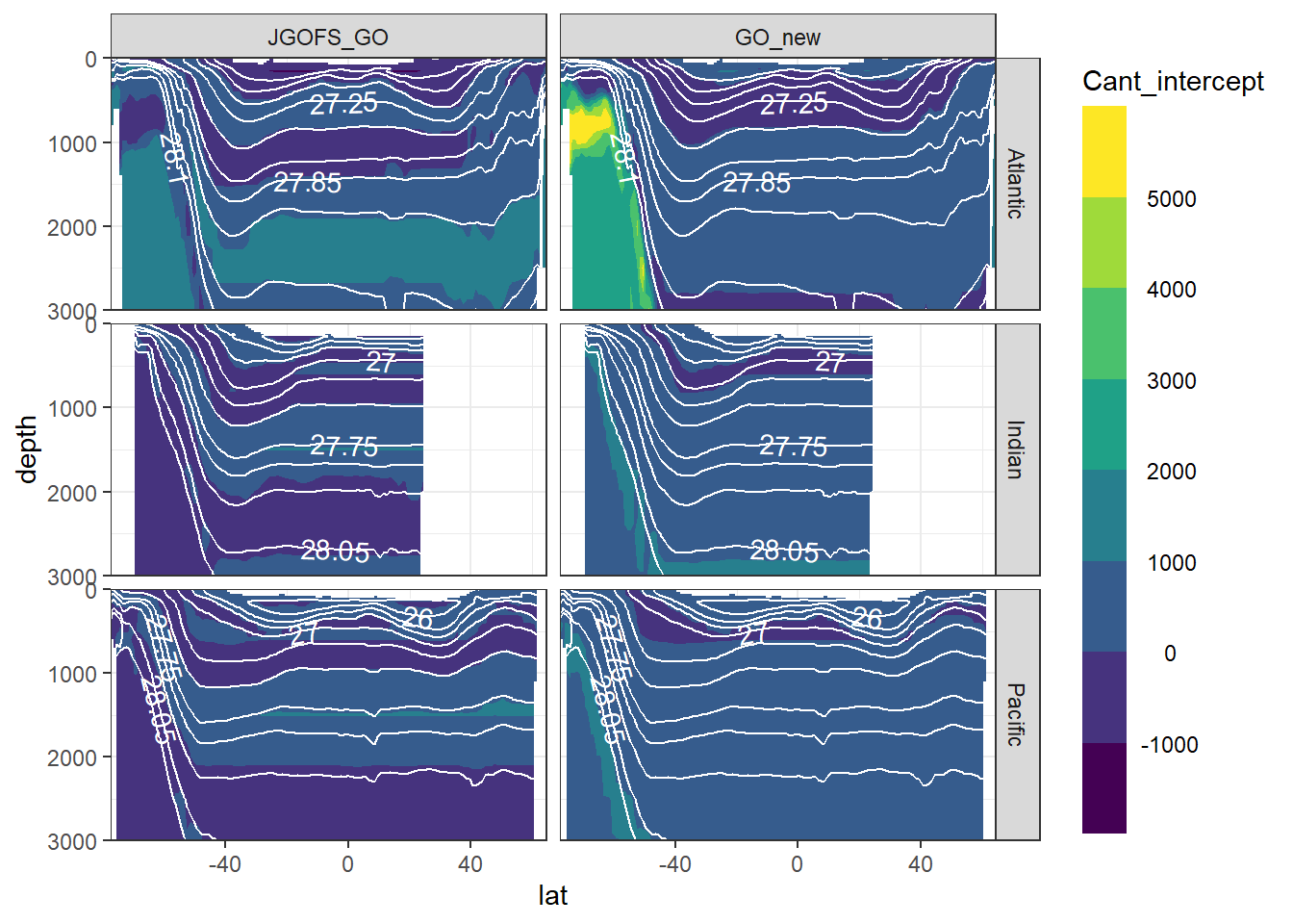
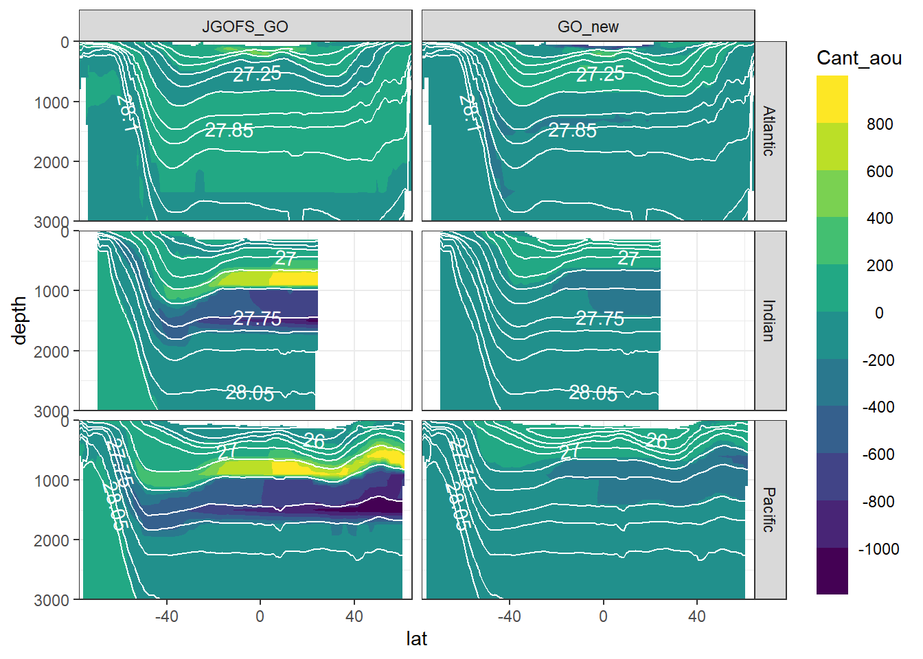
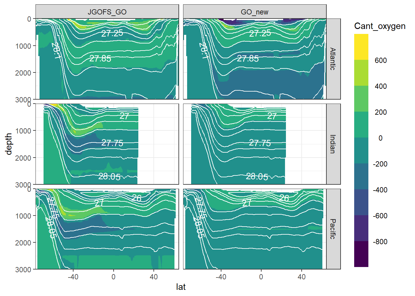
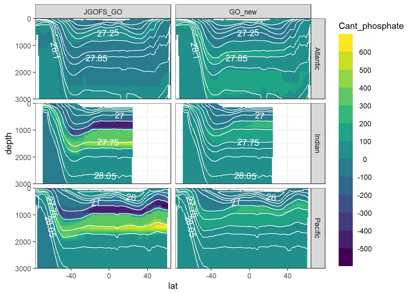
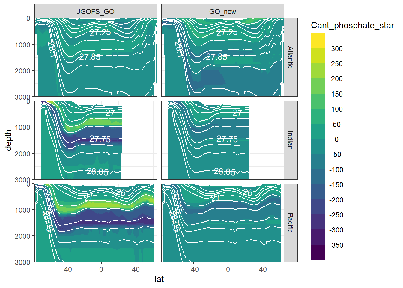
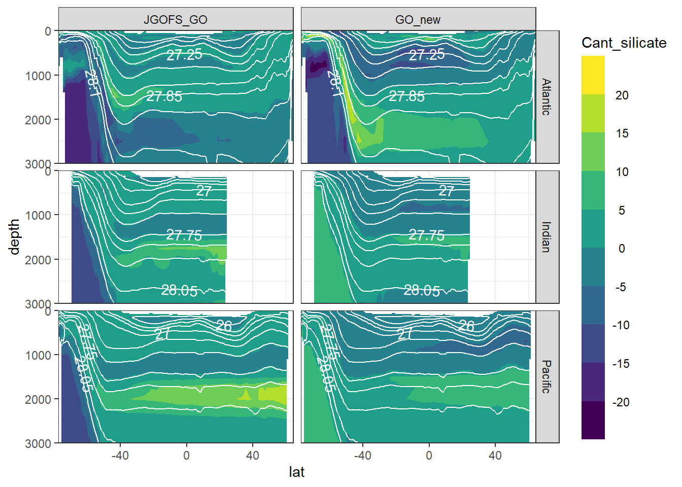
7 Cant - predictor contribution

Cant_predictor_average_zonal <- Cant_predictor_average_zonal %>% 
  mutate(eras = factor(eras, c("JGOFS_GO", "GO_new")))


for (variable in c(
  "Cant_intercept",
  "Cant_aou",
  "Cant_oxygen",
  "Cant_phosphate",
  "Cant_phosphate_star",
  "Cant_silicate",
  "Cant_tem",
  "Cant_sal")) {

print(
section_zonal_average_continous(Cant_predictor_average_zonal,
                                variable,
                                "gamma")
)
    
}

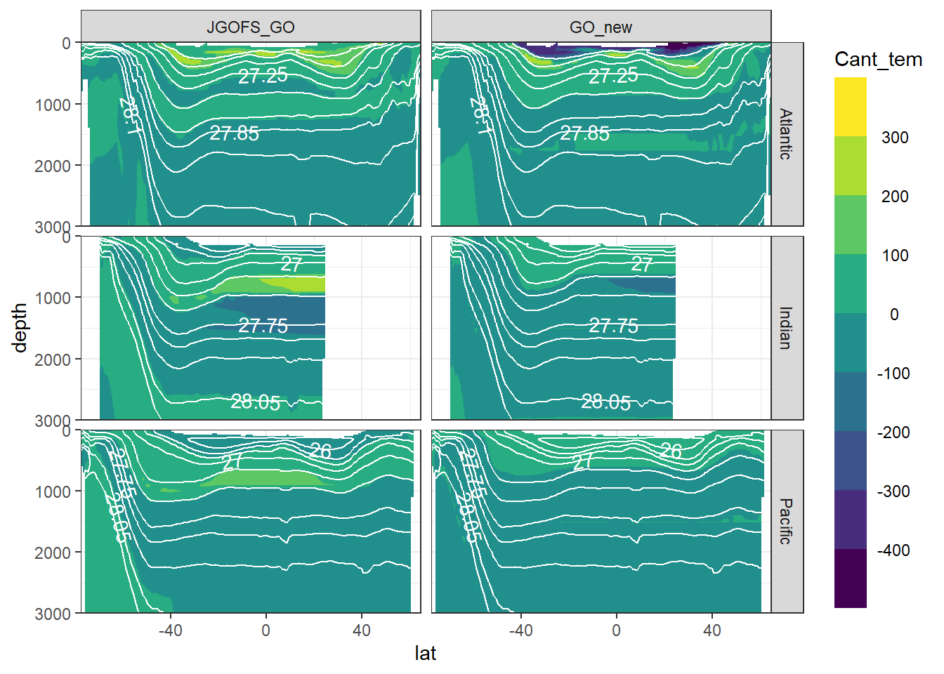
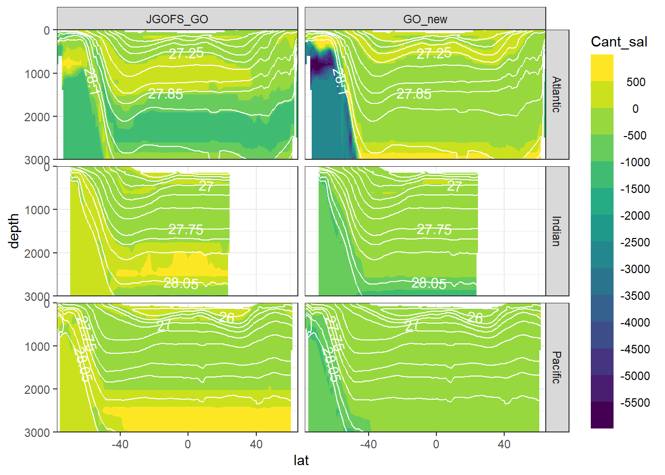
rm(variable)

8 Neutral density

8.1 Slab depth

Please note that:

density slabs covering values >28.1 occur by definition only either in the Atlantic or Indo-Pacific basin
predictor density slabs are only shown for the upper 3000m as used for the mapping, whereas GLODAP observations are displayed for the entire water column as used for fitting eMLRs (in both cases shallow waters are excluded at low density)

gamma_maps <- Cant_average %>% 
  group_by(lat, lon, gamma_slab) %>% 
  summarise(depth_max = max(depth, na.rm = TRUE)) %>% 
  ungroup()

GLODAP_obs_coverage <- GLODAP %>% 
  count(lat, lon, gamma_slab, era) %>% 
  mutate(era = factor(era, c("JGOFS_WOCE", "GO_SHIP", "new_era")))
  
ggplot() +
  geom_raster(data = landmask,
              aes(lon, lat),
              fill = "grey80") +
  geom_raster(data = gamma_maps,
              aes(lon, lat, fill = depth_max)) +
  geom_raster(data = GLODAP_obs_coverage,
              aes(lon, lat), fill = "red") +
  facet_grid(gamma_slab ~ era) +
  coord_quickmap(expand = 0) +
  scale_fill_viridis_c(direction = -1) +
  theme(axis.title = element_blank(),
        axis.ticks = element_blank(),
        axis.text = element_blank(),
        legend.position = "top")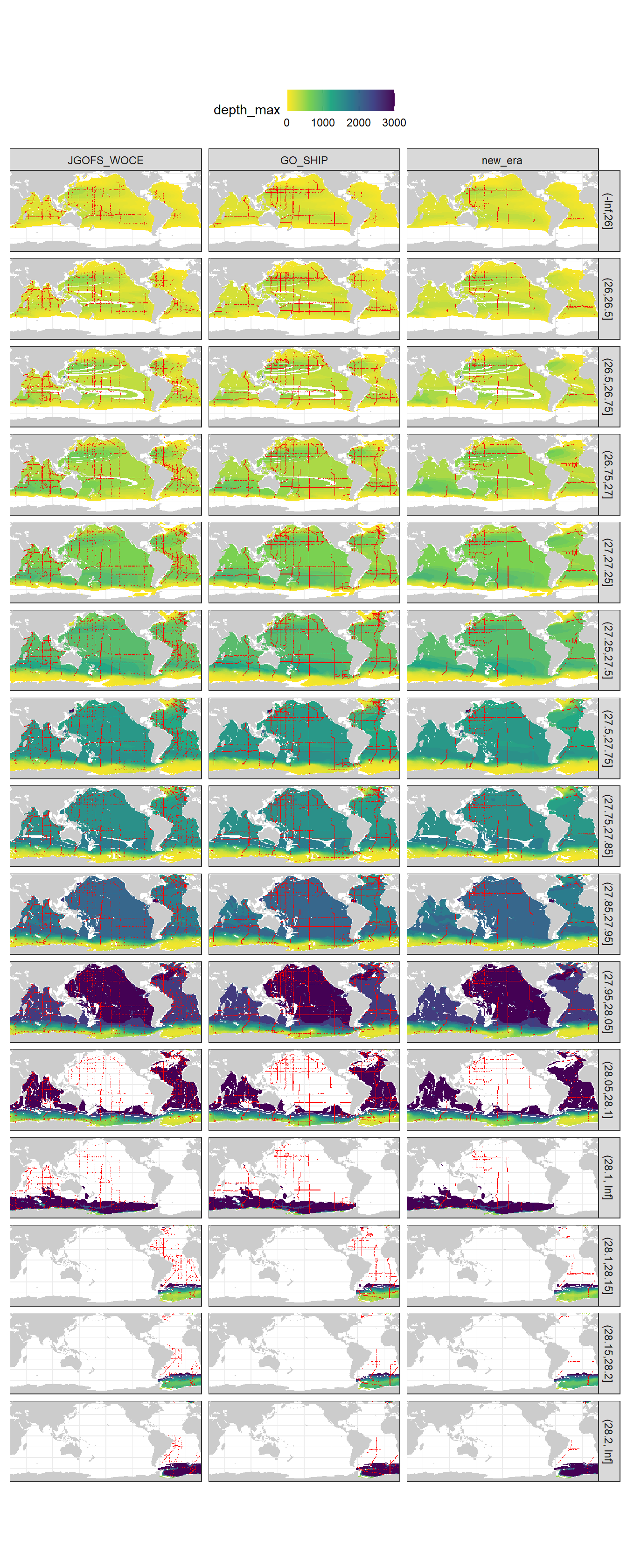

rm(gamma_maps, GLODAP_obs_coverage)

8.2 Surface maps

map_climatology_discrete(Cant_average, "gamma_slab")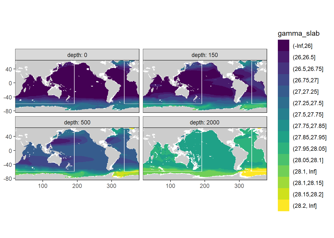

8.3 Zonal sections

The mean zonal distribution of neutral densities was calculated. CAVEAT: Due to practical reasons, binning here does not include the two highest isoneutral density slabs in the Atlantic, yet.

8.3.1 Mean

Cant_average_zonal %>% 
  filter(eras == "JGOFS_GO") %>% 
  ggplot(aes(lat, depth, z = gamma_mean)) +
  geom_contour_filled(breaks = slab_breaks) +
  geom_contour(breaks = slab_breaks,
               col = "white") +
  geom_text_contour(breaks = slab_breaks,
               col = "white",
               skip = 1) +
  scale_fill_viridis_d(name = "Gamma",
                       direction = -1) +
  scale_y_reverse() +
  scale_x_continuous(breaks = seq(-100, 100, 20)) +
  coord_cartesian(expand = 0) +
  guides(fill = guide_colorsteps(barheight = unit(10, "cm"))) +
  facet_grid(basin_AIP~.)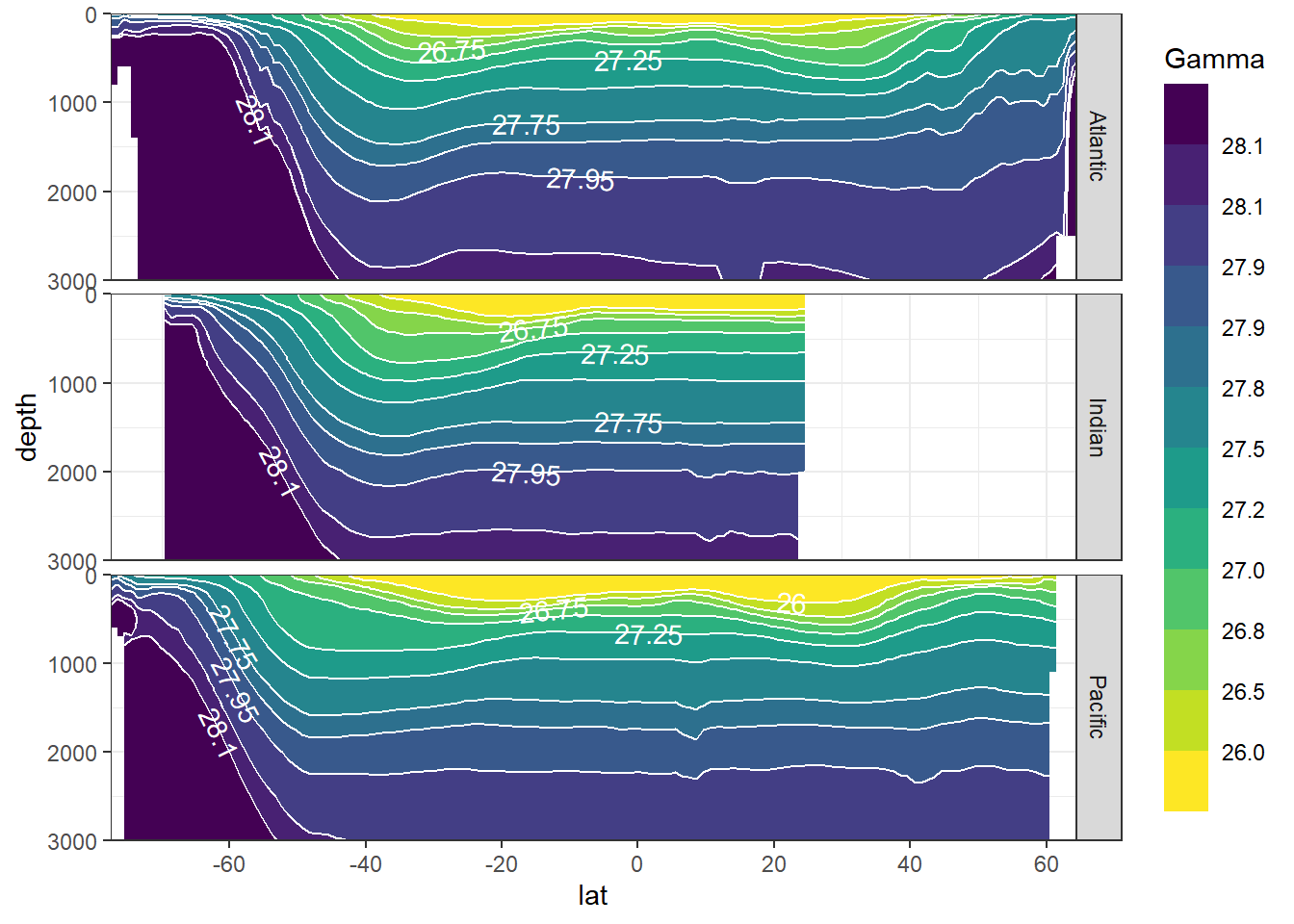

8.3.2 SD

Higher SD of gamma in shallow, subtropical waters results from a more pronounced longitudinal variability.

Cant_average_zonal %>% 
  filter(eras == "JGOFS_GO") %>% 
  ggplot(aes(lat, depth, z = gamma_sd)) +
  geom_contour_filled() +
  scale_fill_viridis_d(name = "Gamma SD",
                       direction = -1) +
  scale_y_reverse() +
  scale_x_continuous(breaks = seq(-100, 100, 20)) +
  coord_cartesian(expand = 0) +
  guides(fill = guide_colorsteps(barheight = unit(10, "cm"))) +
  facet_grid(basin_AIP~.)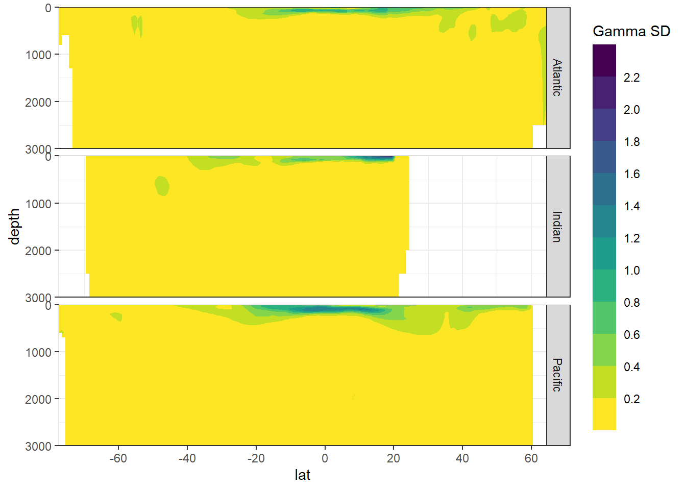

9 Cstar

9.1 Zonal mean sections

Cstar_average_zonal <- Cstar_average_zonal %>% 
    mutate(era = factor(era, c("JGOFS_WOCE", "GO_SHIP", "new_era"))) 

Cstar_average_zonal %>% 
    ggplot(aes(lat, depth, z = Cstar_mean_mean)) +
    geom_contour_filled(bins = 11) +
    scale_fill_viridis_d(name = "Cstar") +
    geom_contour(aes(lat, depth, z = gamma_mean_mean),
                 breaks = slab_breaks,
                 col = "white") +
    geom_text_contour(
      aes(lat, depth, z = gamma_mean_mean),
      breaks = slab_breaks,
      col = "white",
      skip = 1
    ) +
    scale_y_reverse() +
    scale_x_continuous(breaks = seq(-100,100,20)) +
    coord_cartesian(expand = 0) +
    guides(fill = guide_colorsteps(barheight = unit(10, "cm"))) +
    facet_grid(basin_AIP ~ era)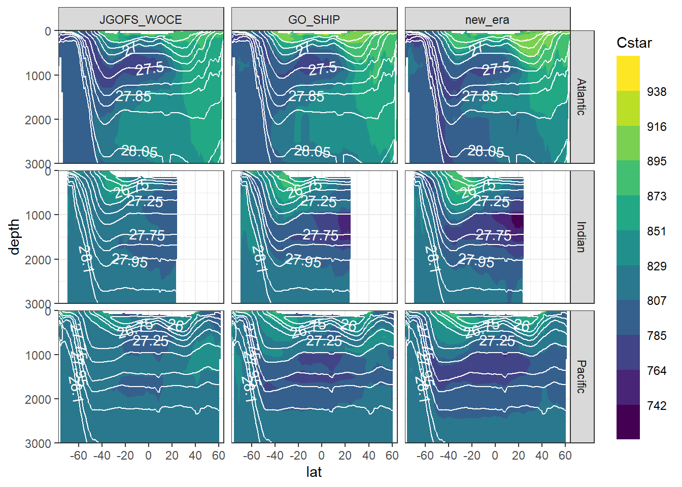

10 Sections by model

Zonal sections plots are produced for every 20° longitude, each era and for all models individually and can be downloaded here.

11 Known issues

Deviations between this study and the results by Gruber et al (2019), short G19, for the same period, might be attributable to following known differences in the implementation of the eMLR(C*) method:

GLODAPv2_2020 here vs an extended version of GLODAPv2 in G19
flagging: Here, we accept f flags 0 and 2 (except for tco2, where only 0 is accepted). G19 claim to use 0 throughout, yet have a high coverage of talk observations in the SE Pacific
Neutral density calculation: Here and in GLODAPv2_2020 a polynomial approximation is used, whereas G19 uses the original Matlab code
Predictor climatology: Here we used WOA18, whereas G19 used WOA13
Missing data in the GLODAP mapped climatology, eg NO3 at surface, where not filled in this study
Cant on neutral density levels calculate as slab mean, rather than on one surface
Here, surface delta Cant were calculated based on Luecker constants, rather than Mehrbach as in G19
Here, pCO2 was calculated from DIC/TA Climatology

sessionInfo()

R version 4.0.2 (2020-06-22)
Platform: x86_64-w64-mingw32/x64 (64-bit)
Running under: Windows 10 x64 (build 18363)

Matrix products: default

locale:
[1] LC_COLLATE=English_Germany.1252  LC_CTYPE=English_Germany.1252   
[3] LC_MONETARY=English_Germany.1252 LC_NUMERIC=C                    
[5] LC_TIME=English_Germany.1252    

attached base packages:
[1] stats     graphics  grDevices utils     datasets  methods   base     

other attached packages:
 [1] threejs_0.3.3    igraph_1.2.5     kableExtra_1.1.0 marelac_2.1.10  
 [5] shape_1.4.4      metR_0.7.0       scales_1.1.1     scico_1.2.0     
 [9] patchwork_1.0.1  forcats_0.5.0    stringr_1.4.0    dplyr_1.0.0     
[13] purrr_0.3.4      readr_1.3.1      tidyr_1.1.0      tibble_3.0.3    
[17] ggplot2_3.3.2    tidyverse_1.3.0  workflowr_1.6.2 

loaded via a namespace (and not attached):
 [1] fs_1.4.2           lubridate_1.7.9    gsw_1.0-5          RColorBrewer_1.1-2
 [5] webshot_0.5.2      httr_1.4.2         rprojroot_1.3-2    tools_4.0.2       
 [9] backports_1.1.8    R6_2.4.1           DBI_1.1.0          colorspace_1.4-1  
[13] sp_1.4-2           withr_2.2.0        tidyselect_1.1.0   compiler_4.0.2    
[17] git2r_0.27.1       cli_2.0.2          rvest_0.3.6        xml2_1.3.2        
[21] isoband_0.2.2      labeling_0.3       checkmate_2.0.0    digest_0.6.25     
[25] rmarkdown_2.3      oce_1.2-0          base64enc_0.1-3    pkgconfig_2.0.3   
[29] htmltools_0.5.0    dbplyr_1.4.4       highr_0.8          htmlwidgets_1.5.1 
[33] rlang_0.4.7        readxl_1.3.1       rstudioapi_0.11    farver_2.0.3      
[37] generics_0.0.2     jsonlite_1.7.0     crosstalk_1.1.0.1  magrittr_1.5      
[41] Rcpp_1.0.5         munsell_0.5.0      fansi_0.4.1        lifecycle_0.2.0   
[45] stringi_1.4.6      whisker_0.4        yaml_2.2.1         plyr_1.8.6        
[49] grid_4.0.2         blob_1.2.1         promises_1.1.1     crayon_1.3.4      
[53] lattice_0.20-41    haven_2.3.1        hms_0.5.3          seacarb_3.2.13    
[57] knitr_1.30         pillar_1.4.6       reprex_0.3.0       glue_1.4.1        
[61] evaluate_0.14      data.table_1.13.0  modelr_0.1.8       vctrs_0.3.2       
[65] httpuv_1.5.4       testthat_2.3.2     cellranger_1.1.0   gtable_0.3.0      
[69] assertthat_0.2.1   xfun_0.16          broom_0.7.0        later_1.1.0.1     
[73] viridisLite_0.3.0  memoise_1.1.0      ellipsis_0.3.1     here_0.1

Analysis of Cant estimates

Jens Daniel Müller

03 November, 2020

1 Data sources

2 Color scale

3 Cant budgets

4 Cant - positive

4.1 Zonal mean sections

4.2 Isoneutral slab distribution

4.3 Inventory map

4.4 Global section

4.4.1 JGOFS_GO

4.4.2 GO_new

5 Cant - all

5.1 Zonal mean sections

5.2 Isoneutral slab distribution

5.3 Inventory map

6 Cant - standard deviation

6.1 Across models

6.2 Across basins

6.3 Correlation

6.3.1 Cant vs model SD

6.3.2 Cant vs regional SD

7 Cant - predictor contribution

8 Neutral density

8.1 Slab depth

8.2 Surface maps

8.3 Zonal sections

8.3.1 Mean

8.3.2 SD

9 Cstar

9.1 Zonal mean sections

10 Sections by model

11 Known issues