Prepare dissolved oxygen data and vertically align to climatology
David Stappard & Jens Daniel Müller
13 May, 2024
Last updated: 2024-05-13
Checks: 7 0
Knit directory:
bgc_argo_r_argodata/analysis/
This reproducible R Markdown analysis was created with workflowr (version 1.7.0). The Checks tab describes the reproducibility checks that were applied when the results were created. The Past versions tab lists the development history.
Great! Since the R Markdown file has been committed to the Git repository, you know the exact version of the code that produced these results.
Great job! The global environment was empty. Objects defined in the global environment can affect the analysis in your R Markdown file in unknown ways. For reproduciblity it’s best to always run the code in an empty environment.
The command set.seed(20211008) was run prior to running
the code in the R Markdown file. Setting a seed ensures that any results
that rely on randomness, e.g. subsampling or permutations, are
reproducible.
Great job! Recording the operating system, R version, and package versions is critical for reproducibility.
Nice! There were no cached chunks for this analysis, so you can be confident that you successfully produced the results during this run.
Great job! Using relative paths to the files within your workflowr project makes it easier to run your code on other machines.
Great! You are using Git for version control. Tracking code development and connecting the code version to the results is critical for reproducibility.
The results in this page were generated with repository version 91e6028. See the Past versions tab to see a history of the changes made to the R Markdown and HTML files.
Note that you need to be careful to ensure that all relevant files for
the analysis have been committed to Git prior to generating the results
(you can use wflow_publish or
wflow_git_commit). workflowr only checks the R Markdown
file, but you know if there are other scripts or data files that it
depends on. Below is the status of the Git repository when the results
were generated:
Ignored files:
    Ignored:    .Rproj.user/

Untracked files:
    Untracked:  analysis/draft.Rmd
    Untracked:  load_argo_core_output.txt

Unstaged changes:
    Deleted:    analysis/MHWs_categorisation.Rmd
    Modified:   analysis/_site.yml
    Modified:   analysis/child/cluster_analysis_base.Rmd
    Modified:   analysis/coverage_maps_North_Atlantic.Rmd
    Modified:   analysis/load_broullon_DIC_TA_clim.Rmd
    Modified:   code/Workflowr_project_managment.R
    Modified:   code/start_background_job.R
    Modified:   code/start_background_job_load.R
    Modified:   code/start_background_job_partial.R
Note that any generated files, e.g. HTML, png, CSS, etc., are not included in this status report because it is ok for generated content to have uncommitted changes.
These are the previous versions of the repository in which changes were
made to the R Markdown
(analysis/doxy_align_climatology.Rmd) and HTML
(docs/doxy_align_climatology.html) files. If you’ve
configured a remote Git repository (see ?wflow_git_remote),
click on the hyperlinks in the table below to view the files as they
were in that past version.
| File | Version | Author | Date | Message |
|---|---|---|---|---|
| html | af6594f | mlarriere | 2024-05-13 | Build site. |
| html | af44bcd | mlarriere | 2024-04-26 | Build site. |
| html | 780276c | mlarriere | 2024-04-19 | Build site. |
| html | f81959a | mlarriere | 2024-04-12 | Build site. |
| html | c076fba | mlarriere | 2024-04-12 | Build site. |
| html | 91f08a6 | mlarriere | 2024-04-07 | Build site. |
| html | db21f55 | mlarriere | 2024-04-06 | Build site. |
| html | 527124f | mlarriere | 2024-03-31 | Build site. |
| Rmd | 1ffb9a4 | mlarriere | 2024-03-31 | doxy_align_climatology building test |
| html | f9de50e | ds2n19 | 2024-01-01 | Build site. |
| html | 07d4eb8 | ds2n19 | 2023-12-20 | Build site. |
| html | fa6cf38 | ds2n19 | 2023-12-14 | Build site. |
| Rmd | 64fd104 | ds2n19 | 2023-12-14 | revised coverage analysis and SO focused cluster analysis. |
Task
This markdown file reads previously created dissolved oxygen climatology file and uses that as the definition of the depth levels that the BGC Argo dissolved oxygen data should be aligned to. Previously created BGC data (bgc_data.rds) and metadata (bgc_metadata.rds) are loaded from the BGC preprocessed folder.
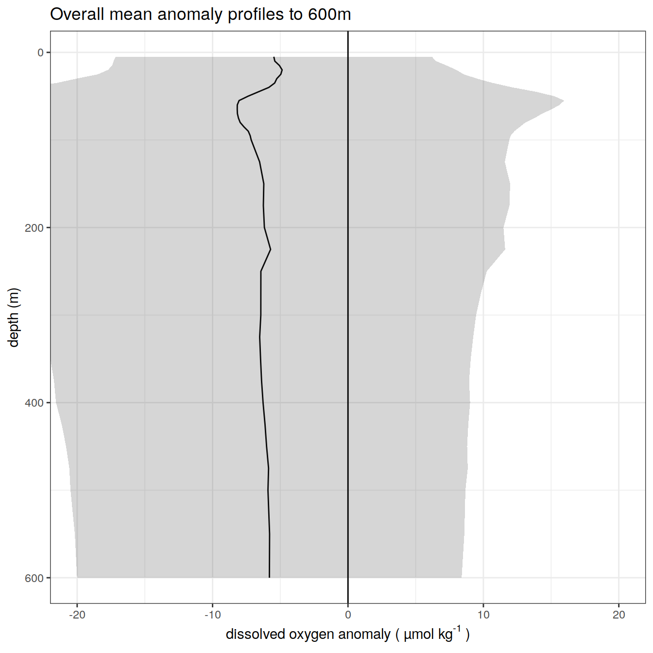
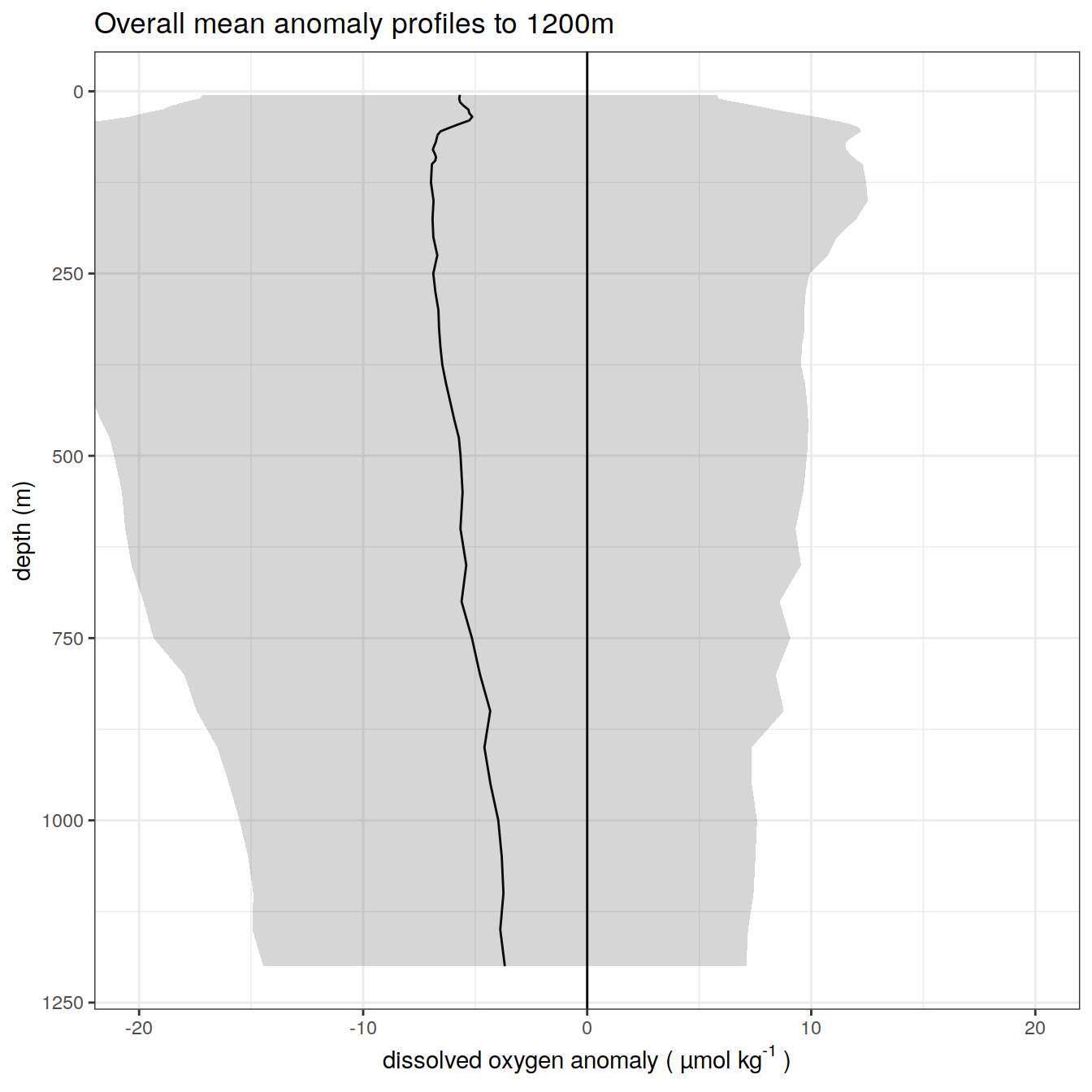
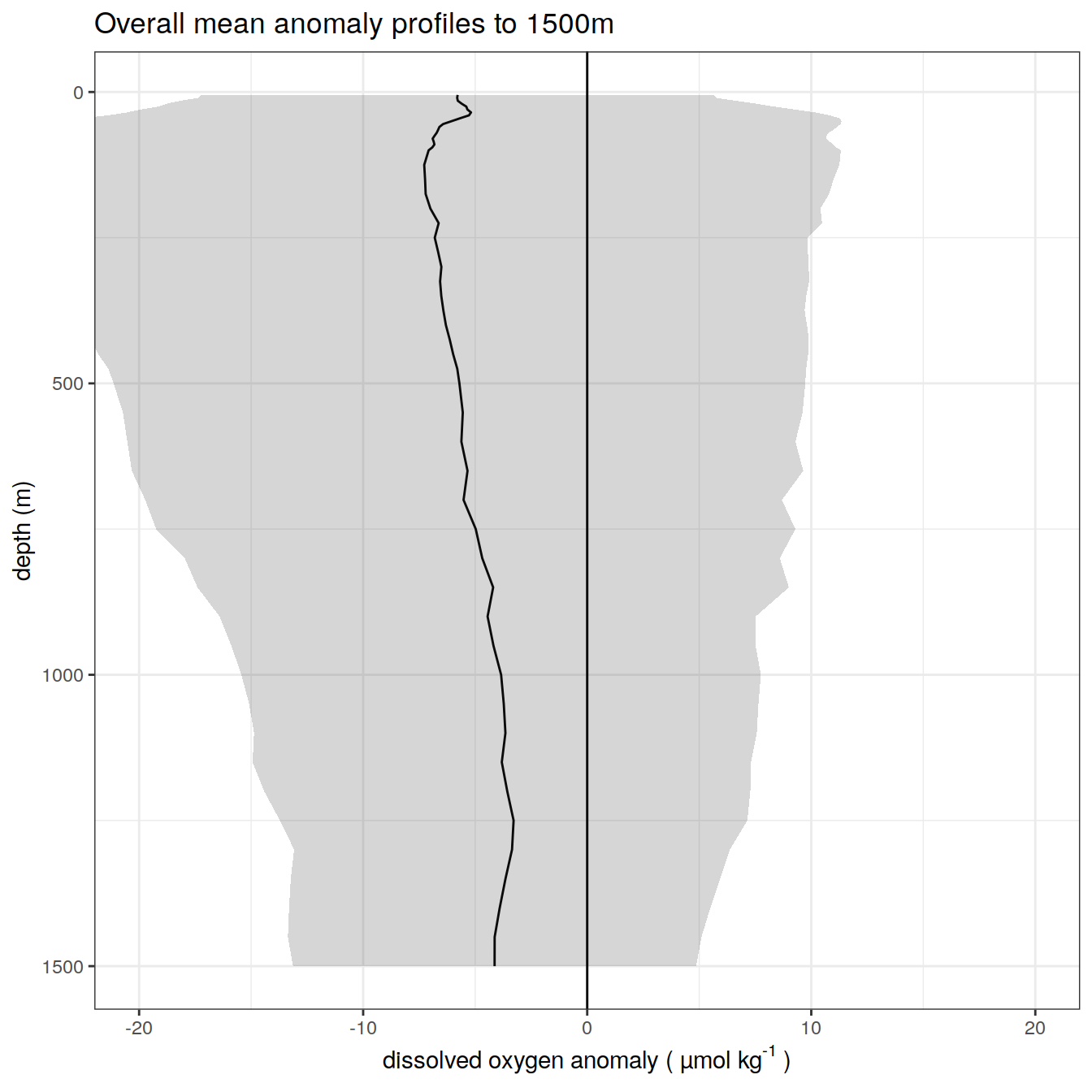
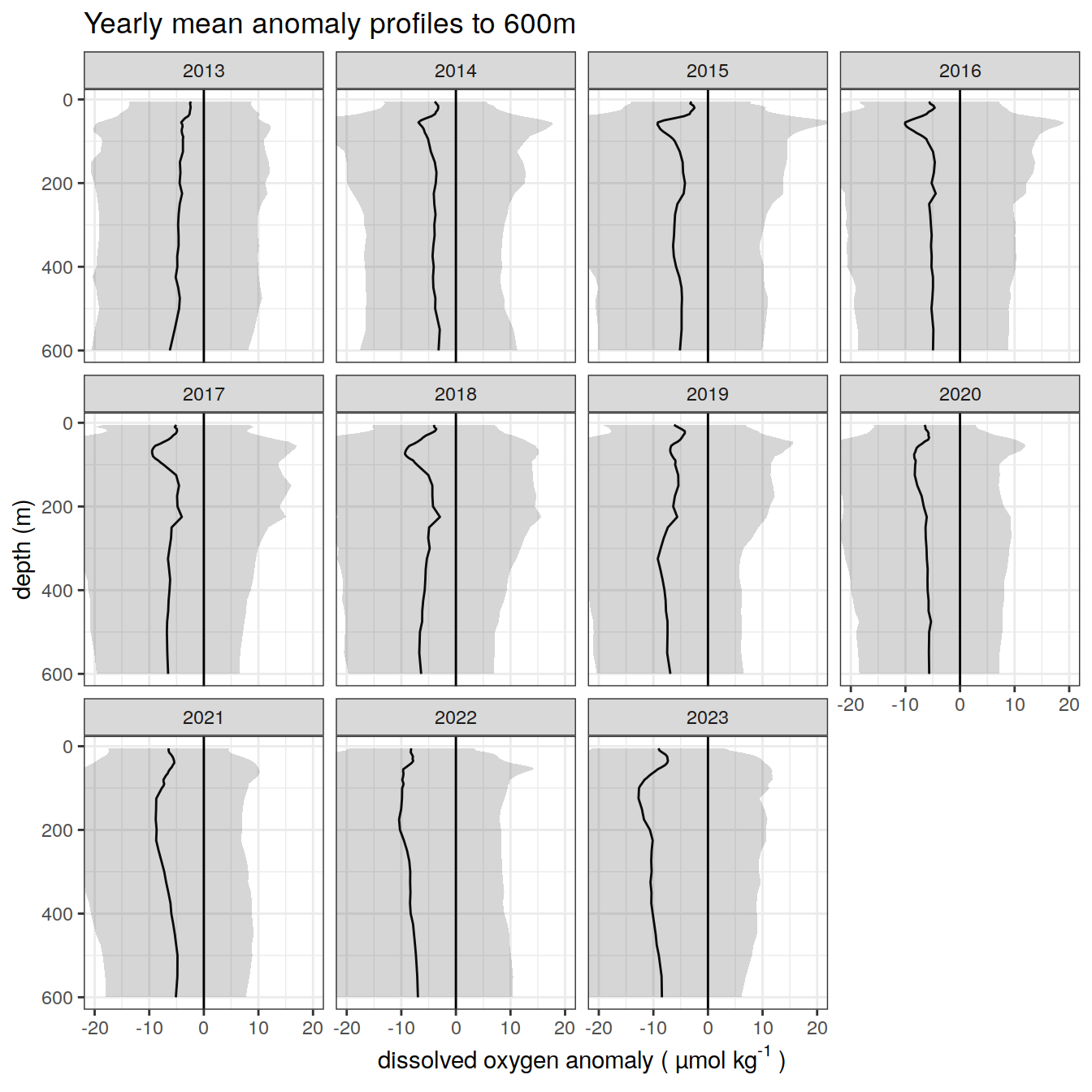
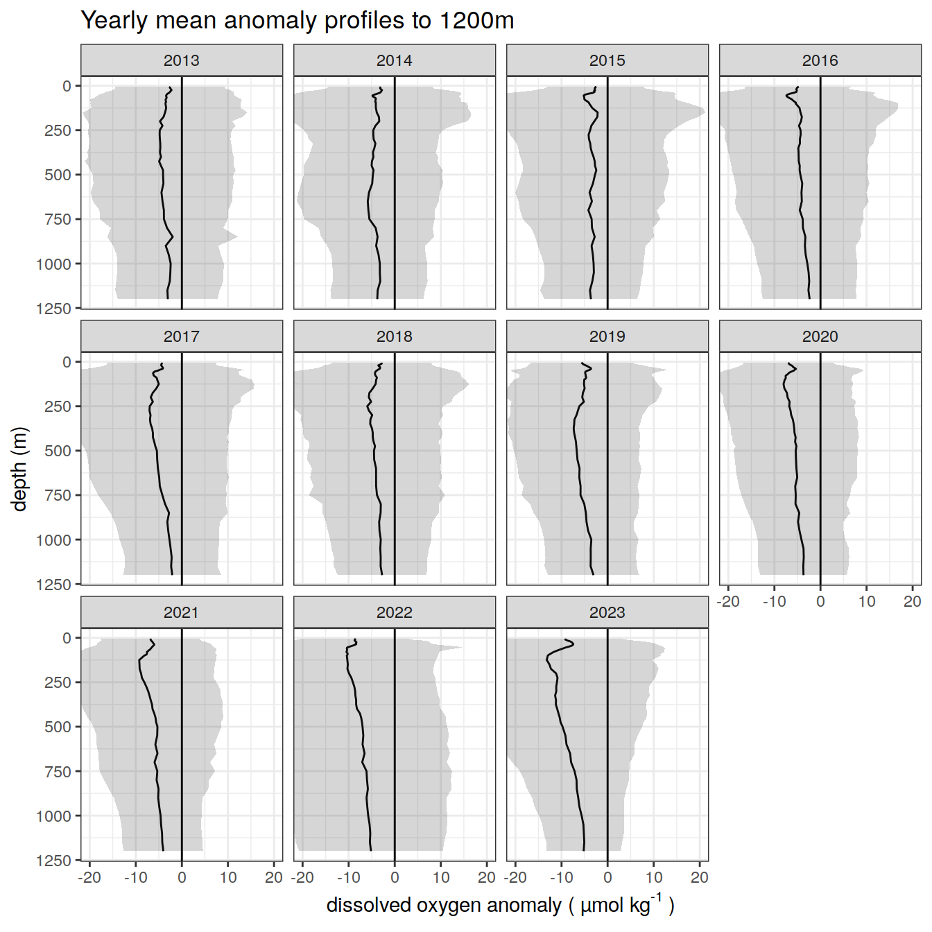
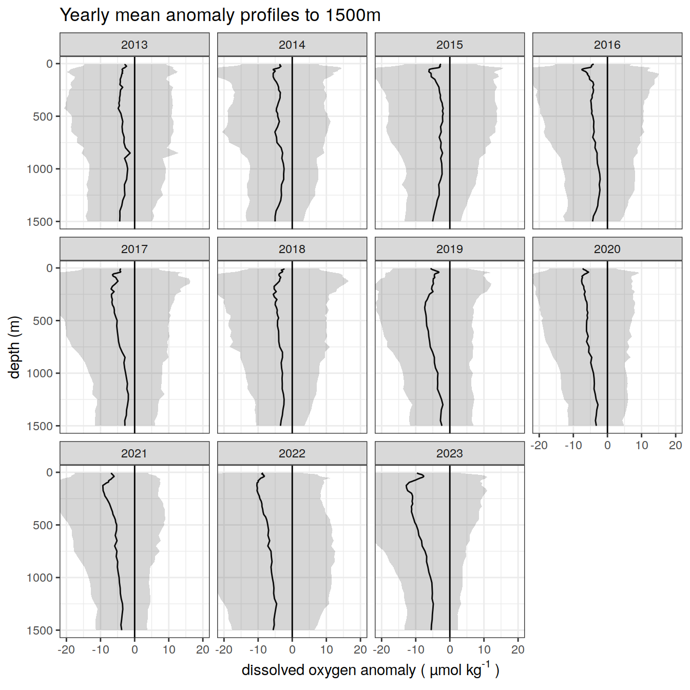
Base data qc flags are checked to ensure that the float position, pressure measurements and dissolved oxygen measurements are good. Pressure is used to derive the depth of each measurement. The dissolved oxygen profile is checked to ensure that significant gaps (specified by the opt_gap_limit, opt_gap_min_depth and opt_gap_max_depth) do not exist. Profiles are assigned a profile_range field that identifies the depth 1 = 600 m, 2 = 1200 m and 3 = 1500 m.
The float dissolved oxygen profiles are then aligned using the spline function to match the depth levels of the climatology resulting in data frame bgc_data_doxy_interpolated_clean. An anomaly file is then created from the vertically aligned profiles and climatology.
Dependencies
woa_doxy_clim.rds - created by load_argo_clim_doxy_woa
bgc_data, bgc_metadata - created by load_argo
Outputs (BGC preprocessed folder)
doxy_bgc_va.rds – vertically aligned dissolved oxygen profiles.
doxy_clim_va.rds – climatology dissolved oxygen profiles.
doxy_anomaly_va.rds – anomaly dissolved oxygen profiles.
Set directories
location of pre-prepared data
Set options
Define options that are used to determine profiles that we will us in the ongoing analysis
# Options

# opt_profile_depth_range
# The profile must have at least one dissolved oxygen reading at a depth <= opt_profile_depth_range[1, ]
# The profile must have at least one dissolved oxygen reading at a depth >= opt_profile_depth_range[2, ].
# In addition if the profile depth does not exceed the min(opt_profile_depth_range[2, ]) (i.e. 600) it will be removed.
profile_range <- c(1, 2, 3)
min_depth <- c(5.0, 5.0, 5.0)
max_depth <- c(600, 1200, 1500)
opt_profile_depth_range <- data.frame(profile_range, min_depth, max_depth)

# opt_gap...
# The profile should not have a gap greater that opt_gap_limit within the range defined by opt_gap_min_depth and opt_gap_max_depth
opt_gap_limit <- c(28, 55, 110)
opt_gap_min_depth <- c(0, 400, 1000)
opt_gap_max_depth <- c(400, 1000, 1500)

# opt_measure_label, opt_xlim and opt_xbreaks are associated with formatting
opt_measure_label <- expression("dissolved oxygen anomaly ( µmol kg"^"-1"~")")
opt_xlim <- c(-20, 20)
opt_xbreaks <- c(-20, -10, 0, 10, 20)

# opt_n_prof_sel
# The selection criteria that is used against n_prof, here set to 1
# Description of n_prof usage is provided at https://argo.ucsd.edu/data/data-faq/version-3-profile-files/ the next two lines are from that page.
#     The main Argo CTD profile is stored in N_PROF=1. All other parameters (including biogeochemical parameters) that are measured
#     with the same vertical sampling scheme and at the same location and time as the main Argo CTD profile are also stored in N_PROF=1.
opt_n_prof_sel = 1

# opt_exclude_shallower
# This option will exclude depths from the climatology and subsequent vertically aligned data that are shallower than opt_exclude_shallower.
# e.g. set to 4.5 to ensure that the top depth of 0.0 m is excluded
# Set to 0.0 to ensure no depths are excluded.
opt_exclude_shallower <- 4.5

# opt_shallow_check_perc and opt_shallow_check_diff
# A check is made to ensure that the pH of the shallowest depth in the profile after vertical alignment is within a limit of the
# pH of the shallowest depth in the profile before vertical alignment
# a opt_shallow_check values of 0.01 results in those with greater than a 1% difference will be reported. Set to 0.0 if percentage check is not required.
# a opt_shallow_report_diff that is non-zero and positive will check that absolute difference. Set to 0.0 if absolute difference check is not required.
opt_shallow_check_perc <- 0.05
opt_shallow_report_perc <- 'profile where shallow check exceeds percentage criteria: '
opt_shallow_check_diff <- 0.5
opt_shallow_report_diff <- 'profile where shallow check exceeds absolute difference criteria: '
read climatology
read dissolved oxygen climatology and prepare to a set range of depths
# climatology values (clim_doxy (°C)) available for lat, lon, month and pressure
woa_doxy_clim <- read_rds(file = paste0(path_argo_preprocessed, '/woa_doxy_clim.rds'))

#What is the max depth we are interested in
opt_profile_max_depth <- max(opt_profile_depth_range$max_depth)

# what are the target depths that we align to
target_depth_levels <- woa_doxy_clim %>% distinct(depth)

target_depth_levels <-
  target_depth_levels %>%
  filter (depth <= opt_profile_max_depth) %>%
  mutate(target_depth = depth) %>%
  select(target_depth)

# select variable of interest and prepare target_depth field
woa_doxy_clim_clean <- woa_doxy_clim %>%
                          select(
                            lat,
                            lon,
                            month,
                            depth,
                            clim_doxy
                          ) %>%
                          mutate(
                            target_depth = depth, .after = depth
                          )

# Exclude 0.0 m depth from the climatology and target_depth_levels
target_depth_levels <- target_depth_levels %>%
  filter(target_depth > opt_exclude_shallower)
woa_doxy_clim_clean <- woa_doxy_clim_clean %>%
  filter(depth > opt_exclude_shallower)

# create all possible combinations of location and month climatologies and depth levels for interpolation
target_depth_grid <-
  expand_grid(target_depth_levels,
              woa_doxy_clim_clean %>% distinct(lat, lon, month))

# extend climatology depth vectors with target depths
woa_doxy_clim_extended <-
  full_join(woa_doxy_clim_clean, target_depth_grid) %>%
  arrange(lat, lon, month, target_depth)


# filter where target depths outside range of climatology depths
# depth is slightly lower than pressure so 1.02 factor is used to ensure bottom value is not lost.
woa_doxy_clim_extended <-
  woa_doxy_clim_extended %>%
  group_by(lat, lon, month) %>%
  filter(
    target_depth <= max(depth, na.rm = TRUE),
    target_depth >= min(depth, na.rm = TRUE)
  ) %>%
  ungroup()

# predict spline interpolation on adjusted depth grid for climatology loaction and month
woa_doxy_clim_interpolated <-
  woa_doxy_clim_extended %>%
  group_by(lat, lon, month) %>%
  mutate(clim_doxy_spline = spline(target_depth, clim_doxy,
                                       method = "natural",
                                       xout = target_depth)$y) %>%
  ungroup()

# subset interpolated values on traget depth grid
woa_doxy_clim_interpolated_clean <-
  inner_join(target_depth_levels, woa_doxy_clim_interpolated)

# select columns and rename to initial names
woa_doxy_clim_interpolated_clean <-
  woa_doxy_clim_interpolated_clean %>%
  select(lat, lon, month,
         depth = target_depth,
         clim_doxy = clim_doxy_spline)

# clean up working tables
rm(woa_doxy_clim_clean, woa_doxy_clim_extended, woa_doxy_clim_interpolated)
read doxy data
read dissolved oxygen profile and carry out basic checks, good data.
Profile limits
Apply the rules that are determined by options set in set_options. Profile must cover a set range and not contain gaps.
Vertical align doxy
We have a set of dissolved oxygen profiles that match our criteria we now need to align that data set to match the depth that are in target_depth_levels, this will match the range of climatology values in woa_doxy_clim_interpolated_clean
Check shallow
A check is made that the shallowest doxy value after the vertical alignment is within a specified percentage of the shallowest doxy value before the vertical alignment
# Combined dataframe with shallow value pre and post vertical alignment
shallow_doxy_check <-
  full_join(shallow_doxy_raw, shallow_doxy_va)

# Determine those profile that are outside of percentage criteria.
if (opt_shallow_check_perc > 0.0){
  shallow_check_report <- shallow_doxy_check %>%
    filter (abs((doxy_shallow_raw - doxy_shallow_va) / doxy_shallow_raw) > opt_shallow_check_perc)

  # Write issues to console
  if (nrow(shallow_check_report) > 0) {
    print (opt_shallow_report_perc)
    shallow_check_report %>% rmarkdown::paged_table()
  }
}

# Determine those profile that are outside of absolute difference criteria.
if (opt_shallow_check_diff > 0.0){
  shallow_check_report <- shallow_doxy_check %>%
    filter (abs(doxy_shallow_raw - doxy_shallow_va) > opt_shallow_check_diff)

  # Write issues to console
  if (nrow(shallow_check_report) > 0) {
    print (opt_shallow_report_diff)
    shallow_check_report %>% rmarkdown::paged_table()
  }
}


# remove working files
rm(shallow_doxy_check, shallow_doxy_raw, shallow_doxy_va, shallow_check_report)
gc()
Create anomaly profiles
Create anomaly profiles as observed - climatology
# Create bgc_doxy_anomaly, but only where we have an climatology dissolved oxygen
bgc_doxy_anomaly <-
  inner_join(bgc_data_doxy_interpolated_clean, woa_doxy_clim_interpolated_clean)

# Calculate the anomaly dissolved oxygen
bgc_doxy_anomaly <- bgc_doxy_anomaly %>%
                      mutate(
                        anomaly = doxy - clim_doxy
                      )

# -----------------------------------------------------------------------------
# Climatology check
# -----------------------------------------------------------------------------
# It is possible even though we have observational measures to full depth the climatology may not matach all depth.
# These profiles will be removed from both doxy_bgc_va and doxy_anomaly_va

# Anomaly max depth
bgc_doxy_anomaly_depth_check <- bgc_doxy_anomaly %>%
  group_by(file_id,
           profile_range) %>%
  summarise(min_pdepth = min(depth),
            max_pdepth = max(depth)) %>%
  ungroup()

# Add the required min depth and max depth
bgc_doxy_anomaly_depth_check <- left_join(bgc_doxy_anomaly_depth_check, opt_profile_depth_range)

# This profiles do not match the depth required by the profile_range
# min_depth_check <- min(target_depth_grid$target_depth)

# Please double check if the criterion should be
# each profile is checked against the min depth specified in min_depth
# max depth specified in max_depth.
remove_profiles <- bgc_doxy_anomaly_depth_check %>%
  filter((max_pdepth < max_depth) | (min_pdepth > min_depth)) %>%
  distinct(file_id)

# remove from both bgc_data_doxy_interpolated_clean and bgc_doxy_anomaly
bgc_data_doxy_interpolated_clean <-
  anti_join(bgc_data_doxy_interpolated_clean, remove_profiles)

bgc_doxy_anomaly <- anti_join(bgc_doxy_anomaly, remove_profiles)
Write files
Write the climatology that maps onto depth levels, interpolated dissolved oxygen profiles that map onto depth levels and resulting anomaly files.
# Write files
bgc_data_doxy_interpolated_clean %>%
  write_rds(file = paste0(path_argo_preprocessed, "/doxy_bgc_va.rds"))

woa_doxy_clim_interpolated_clean %>%
  write_rds(file = paste0(path_argo_preprocessed, "/doxy_clim_va.rds"))

bgc_doxy_anomaly %>%
  write_rds(file = paste0(path_argo_preprocessed, "/doxy_anomaly_va.rds"))

# Rename so that names match if just reading existing files
doxy_bgc_va <- bgc_data_doxy_interpolated_clean
doxy_clim_va <- woa_doxy_clim_interpolated_clean
doxy_anomaly_va <- bgc_doxy_anomaly

#rm(bgc_data_doxy_interpolated_clean, woa_doxy_clim_interpolated_clean, bgc_doxy_anomaly)
read files
Read files that were previously created ready for analysis
# read files
doxy_bgc_va <- read_rds(file = paste0(path_argo_preprocessed, "/doxy_bgc_va.rds"))

doxy_clim_va <- read_rds(file = paste0(path_argo_preprocessed, "/doxy_clim_va.rds"))

doxy_anomaly_va <- read_rds(file = paste0(path_argo_preprocessed, "/doxy_anomaly_va.rds"))
Analysis
dissolved oxygen anomaly
Details of mean anomaly over analysis period
max_depth_1 <- opt_profile_depth_range[1, "max_depth"]
max_depth_2 <- opt_profile_depth_range[2, "max_depth"]
max_depth_3 <- opt_profile_depth_range[3, "max_depth"]

# Profiles to 600m
anomaly_overall_mean_1 <- doxy_anomaly_va %>%
  filter(profile_range %in% c(1, 2, 3) & depth <= max_depth_1) %>%
  group_by(depth) %>%
  summarise(doxy_count = n(),
            doxy_anomaly_mean = mean(anomaly, na.rm = TRUE),
            doxy_anomaly_sd = sd(anomaly, na.rm = TRUE))

anomaly_year_mean_1 <- doxy_anomaly_va %>%
  filter(profile_range %in% c(1, 2, 3) & depth <= max_depth_1) %>%
  group_by(year, depth) %>%
  summarise(doxy_count = n(),
            doxy_anomaly_mean = mean(anomaly, na.rm = TRUE),
            doxy_anomaly_sd = sd(anomaly, na.rm = TRUE))

# Profiles to 1200m
anomaly_overall_mean_2 <- doxy_anomaly_va %>%
  filter(profile_range %in% c(2, 3) & depth <= max_depth_2) %>%
  group_by(depth) %>%
  summarise(doxy_count = n(),
            doxy_anomaly_mean = mean(anomaly, na.rm = TRUE),
            doxy_anomaly_sd = sd(anomaly, na.rm = TRUE))

anomaly_year_mean_2 <- doxy_anomaly_va %>%
  filter(profile_range %in% c(2, 3) & depth <= max_depth_2) %>%
  group_by(year, depth) %>%
  summarise(doxy_count = n(),
            doxy_anomaly_mean = mean(anomaly, na.rm = TRUE),
            doxy_anomaly_sd = sd(anomaly, na.rm = TRUE))

# Profiles to 1500m
anomaly_overall_mean_3 <- doxy_anomaly_va %>%
  filter(profile_range %in% c(3) & depth <= max_depth_3) %>%
  group_by(depth) %>%
  summarise(doxy_count = n(),
            doxy_anomaly_mean = mean(anomaly, na.rm = TRUE),
            doxy_anomaly_sd = sd(anomaly, na.rm = TRUE))

anomaly_year_mean_3 <- doxy_anomaly_va %>%
  filter(profile_range %in% c(3) & depth <= max_depth_3) %>%
  group_by(year, depth) %>%
  summarise(doxy_count = n(),
            doxy_anomaly_mean = mean(anomaly, na.rm = TRUE),
            doxy_anomaly_sd = sd(anomaly, na.rm = TRUE))

# All years anomaly
anomaly_overall_mean_1 %>%
  ggplot()+
  geom_path(aes(x = doxy_anomaly_mean,
                y = depth))+
  geom_ribbon(aes(xmax = doxy_anomaly_mean + doxy_anomaly_sd,
                  xmin = doxy_anomaly_mean - doxy_anomaly_sd,
                  y = depth),
              alpha = 0.2)+
  geom_vline(xintercept = 0)+
  scale_y_reverse() +
  coord_cartesian(xlim = opt_xlim) +
  scale_x_continuous(breaks = opt_xbreaks) +
  labs(
    title = paste0('Overall mean anomaly profiles to ', max_depth_1, 'm'),
    x = opt_measure_label,
    y = 'depth (m)'
  )
anomaly_overall_mean_2 %>%
  ggplot()+
  geom_path(aes(x = doxy_anomaly_mean,
                y = depth))+
  geom_ribbon(aes(xmax = doxy_anomaly_mean + doxy_anomaly_sd,
                  xmin = doxy_anomaly_mean - doxy_anomaly_sd,
                  y = depth),
              alpha = 0.2)+
  geom_vline(xintercept = 0)+
  scale_y_reverse() +
  coord_cartesian(xlim = opt_xlim) +
  scale_x_continuous(breaks = opt_xbreaks) +
  labs(
    title = paste0('Overall mean anomaly profiles to ', max_depth_2, 'm'),
    x = opt_measure_label,
    y = 'depth (m)'
  )
anomaly_overall_mean_3 %>%
  ggplot()+
  geom_path(aes(x = doxy_anomaly_mean,
                y = depth))+
  geom_ribbon(aes(xmax = doxy_anomaly_mean + doxy_anomaly_sd,
                  xmin = doxy_anomaly_mean - doxy_anomaly_sd,
                  y = depth),
              alpha = 0.2)+
  geom_vline(xintercept = 0)+
  scale_y_reverse() +
  coord_cartesian(xlim = opt_xlim) +
  scale_x_continuous(breaks = opt_xbreaks) +
  labs(
    title = paste0('Overall mean anomaly profiles to ', max_depth_3, 'm'),
    x = opt_measure_label,
    y = 'depth (m)'
  )
# yearly anomaly
anomaly_year_mean_1 %>%
  ggplot()+
  geom_path(aes(x = doxy_anomaly_mean,
                y = depth))+
  geom_ribbon(aes(xmax = doxy_anomaly_mean + doxy_anomaly_sd,
                  xmin = doxy_anomaly_mean - doxy_anomaly_sd,
                  y = depth),
              alpha = 0.2)+
  geom_vline(xintercept = 0)+
  scale_y_reverse() +
  facet_wrap(~year)+
  coord_cartesian(xlim = opt_xlim) +
  scale_x_continuous(breaks = opt_xbreaks) +
  labs(
    title = paste0('Yearly mean anomaly profiles to ', max_depth_1, 'm'),
    x = opt_measure_label,
    y = 'depth (m)'
  )
anomaly_year_mean_2 %>%
  ggplot()+
  geom_path(aes(x = doxy_anomaly_mean,
                y = depth))+
  geom_ribbon(aes(xmax = doxy_anomaly_mean + doxy_anomaly_sd,
                  xmin = doxy_anomaly_mean - doxy_anomaly_sd,
                  y = depth),
              alpha = 0.2)+
  geom_vline(xintercept = 0)+
  scale_y_reverse() +
  facet_wrap(~year)+
  coord_cartesian(xlim = opt_xlim) +
  scale_x_continuous(breaks = opt_xbreaks) +
  labs(
    title = paste0('Yearly mean anomaly profiles to ', max_depth_2, 'm'),
    x = opt_measure_label,
    y = 'depth (m)'
  )
anomaly_year_mean_3 %>%
  ggplot()+
  geom_path(aes(x = doxy_anomaly_mean,
                y = depth))+
  geom_ribbon(aes(xmax = doxy_anomaly_mean + doxy_anomaly_sd,
                  xmin = doxy_anomaly_mean - doxy_anomaly_sd,
                  y = depth),
              alpha = 0.2)+
  geom_vline(xintercept = 0)+
  scale_y_reverse() +
  facet_wrap(~year)+
  coord_cartesian(xlim = opt_xlim) +
  scale_x_continuous(breaks = opt_xbreaks) +
  labs(
    title = paste0('Yearly mean anomaly profiles to ', max_depth_3, 'm'),
    x = opt_measure_label,
    y = 'depth (m)'
  )
#rm(anomaly_overall_mean)Profile counts
Details of the number of profiles and to which depths over the analysis period
doxy_histogram <- doxy_bgc_va %>%
  group_by(year, profile_range = as.character(profile_range)) %>%
  summarise(num_profiles = n_distinct(file_id)) %>%
  ungroup()

doxy_histogram %>%
  ggplot() +
  geom_bar(
    aes(
      x = year,
      y = num_profiles,
      fill = profile_range,
      group = profile_range
    ),
    position = "stack",
    stat = "identity"
  ) +
  scale_fill_viridis_d() +
  labs(title = "dissolved oxygen profiles per year and profile range",
       x = "year",
       y = "profile count",
       fill = "profile range")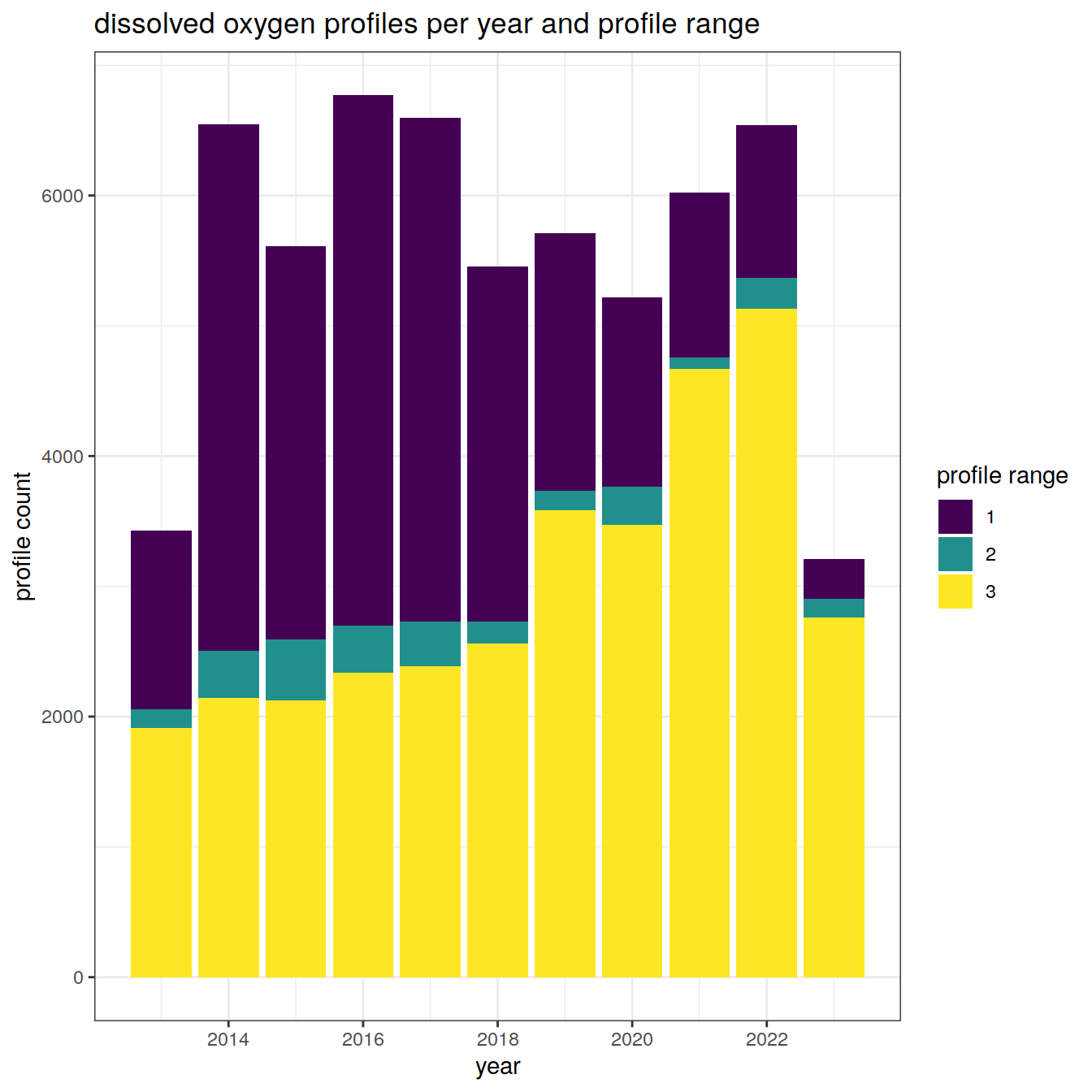
sessionInfo()R version 4.2.2 (2022-10-31)
Platform: x86_64-pc-linux-gnu (64-bit)
Running under: openSUSE Leap 15.5
Matrix products: default
BLAS: /usr/local/R-4.2.2/lib64/R/lib/libRblas.so
LAPACK: /usr/local/R-4.2.2/lib64/R/lib/libRlapack.so
locale:
[1] LC_CTYPE=en_US.UTF-8 LC_NUMERIC=C
[3] LC_TIME=en_US.UTF-8 LC_COLLATE=en_US.UTF-8
[5] LC_MONETARY=en_US.UTF-8 LC_MESSAGES=en_US.UTF-8
[7] LC_PAPER=en_US.UTF-8 LC_NAME=C
[9] LC_ADDRESS=C LC_TELEPHONE=C
[11] LC_MEASUREMENT=en_US.UTF-8 LC_IDENTIFICATION=C
attached base packages:
[1] stats graphics grDevices utils datasets methods base
other attached packages:
[1] ggforce_0.4.1 gsw_1.1-1 gridExtra_2.3 lubridate_1.9.0
[5] timechange_0.1.1 argodata_0.1.0 forcats_0.5.2 stringr_1.5.0
[9] dplyr_1.1.3 purrr_1.0.2 readr_2.1.3 tidyr_1.3.0
[13] tibble_3.2.1 ggplot2_3.4.4 tidyverse_1.3.2 workflowr_1.7.0
loaded via a namespace (and not attached):
[1] httr_1.4.4 sass_0.4.4 viridisLite_0.4.1
[4] jsonlite_1.8.3 modelr_0.1.10 bslib_0.4.1
[7] assertthat_0.2.1 getPass_0.2-2 highr_0.9
[10] googlesheets4_1.0.1 cellranger_1.1.0 yaml_2.3.6
[13] pillar_1.9.0 backports_1.4.1 glue_1.6.2
[16] digest_0.6.30 promises_1.2.0.1 polyclip_1.10-4
[19] rvest_1.0.3 colorspace_2.0-3 htmltools_0.5.8.1
[22] httpuv_1.6.6 pkgconfig_2.0.3 broom_1.0.5
[25] haven_2.5.1 scales_1.2.1 processx_3.8.0
[28] tweenr_2.0.2 whisker_0.4 later_1.3.0
[31] tzdb_0.3.0 git2r_0.30.1 googledrive_2.0.0
[34] farver_2.1.1 generics_0.1.3 ellipsis_0.3.2
[37] cachem_1.0.6 withr_2.5.0 cli_3.6.1
[40] magrittr_2.0.3 crayon_1.5.2 readxl_1.4.1
[43] evaluate_0.18 ps_1.7.2 fs_1.5.2
[46] fansi_1.0.3 MASS_7.3-58.1 xml2_1.3.3
[49] tools_4.2.2 hms_1.1.2 gargle_1.2.1
[52] lifecycle_1.0.3 munsell_0.5.0 reprex_2.0.2
[55] callr_3.7.3 compiler_4.2.2 jquerylib_0.1.4
[58] RNetCDF_2.6-1 rlang_1.1.1 grid_4.2.2
[61] rstudioapi_0.15.0 labeling_0.4.2 rmarkdown_2.18
[64] gtable_0.3.1 DBI_1.2.2 R6_2.5.1
[67] knitr_1.41 fastmap_1.1.0 utf8_1.2.2
[70] rprojroot_2.0.3 stringi_1.7.8 Rcpp_1.0.10
[73] vctrs_0.6.4 dbplyr_2.2.1 tidyselect_1.2.0
[76] xfun_0.35