Number of BGC-Argo observations
Pasqualina Vonlanthen & Jens Daniel Müller
19 October, 2021
Last updated: 2021-10-19
Checks: 7 0
Knit directory: bgc_argo_r_argodata/
This reproducible R Markdown analysis was created with workflowr (version 1.6.2). The Checks tab describes the reproducibility checks that were applied when the results were created. The Past versions tab lists the development history.
Great! Since the R Markdown file has been committed to the Git repository, you know the exact version of the code that produced these results.
Great job! The global environment was empty. Objects defined in the global environment can affect the analysis in your R Markdown file in unknown ways. For reproduciblity it’s best to always run the code in an empty environment.
The command set.seed(20211008) was run prior to running the code in the R Markdown file. Setting a seed ensures that any results that rely on randomness, e.g. subsampling or permutations, are reproducible.
Great job! Recording the operating system, R version, and package versions is critical for reproducibility.
Nice! There were no cached chunks for this analysis, so you can be confident that you successfully produced the results during this run.
Great job! Using relative paths to the files within your workflowr project makes it easier to run your code on other machines.
Great! You are using Git for version control. Tracking code development and connecting the code version to the results is critical for reproducibility.
The results in this page were generated with repository version f460b9a. See the Past versions tab to see a history of the changes made to the R Markdown and HTML files.
Note that you need to be careful to ensure that all relevant files for the analysis have been committed to Git prior to generating the results (you can use wflow_publish or wflow_git_commit). workflowr only checks the R Markdown file, but you know if there are other scripts or data files that it depends on. Below is the status of the Git repository when the results were generated:
Ignored files:
    Ignored:    .Rhistory
    Ignored:    .Rproj.user/

Unstaged changes:
    Modified:   code/Workflowr_project_managment.R
Note that any generated files, e.g. HTML, png, CSS, etc., are not included in this status report because it is ok for generated content to have uncommitted changes.
These are the previous versions of the repository in which changes were made to the R Markdown (analysis/count_observations.Rmd) and HTML (docs/count_observations.html) files. If you’ve configured a remote Git repository (see ?wflow_git_remote), click on the hyperlinks in the table below to view the files as they were in that past version.
| File | Version | Author | Date | Message |
|---|---|---|---|---|
| Rmd | f460b9a | jens-daniel-mueller | 2021-10-19 | code review jens |
| html | 8d44223 | pasqualina-vonlanthendinenna | 2021-10-15 | Build site. |
| Rmd | 0c2a0da | pasqualina-vonlanthendinenna | 2021-10-15 | tried to change list format |
| html | ab5b7a3 | pasqualina-vonlanthendinenna | 2021-10-15 | Build site. |
| Rmd | 50a56d5 | pasqualina-vonlanthendinenna | 2021-10-15 | tried to change list format |
| html | 0719903 | pasqualina-vonlanthendinenna | 2021-10-15 | Build site. |
| Rmd | 972c86f | pasqualina-vonlanthendinenna | 2021-10-15 | tried to change list format |
| html | c3be663 | pasqualina-vonlanthendinenna | 2021-10-15 | Build site. |
| Rmd | e08cc84 | pasqualina-vonlanthendinenna | 2021-10-15 | changed title sizes in timeseries doc |
| html | 83724a0 | pasqualina-vonlanthendinenna | 2021-10-14 | Build site. |
| html | 5331669 | pasqualina-vonlanthendinenna | 2021-10-13 | Build site. |
| Rmd | d8616e1 | pasqualina-vonlanthendinenna | 2021-10-13 | added timeseries of all 3 bgc variables |
| html | 795b5ad | pasqualina-vonlanthendinenna | 2021-10-13 | Build site. |
| Rmd | 81f5ac9 | pasqualina-vonlanthendinenna | 2021-10-13 | added timeseries of all 3 bgc variables |
| html | 4840e49 | pasqualina-vonlanthendinenna | 2021-10-12 | Build site. |
| Rmd | 2fb35f7 | pasqualina-vonlanthendinenna | 2021-10-12 | added reading data in page |
Task
Count the number of bgc-argo observations, and plot the evolution over time.
Load data
Read the files created in loading_data.html:
argo_set_cache_dir('/nfs/kryo/work/updata/bgc_argo_r_argodata')

argo_update_global(max_global_cache_age = Inf)
argo_update_data(max_data_cache_age = Inf) # the arguments max_global_cache_age and max_data_cache_age indicate the age of the cached files to update (in hours) (Inf means always use the cached file, and -Inf means always download from the server)
# e.g. if max_global_cache_age = 5, then files older than 5 hours will be updated


bgc_subset = argo_global_synthetic_prof() %>%
  argo_filter_data_mode(data_mode = 'delayed') %>%
  argo_filter_date(date_min = '2013-01-01',
                   date_max = '2015-12-31') # download bgc-argo files containing delayed-mode data (recommended for bgc variables) between January 1, 2013 and December 31, 2015 (selects this specific subset of the cached files)

# check the dates
# max(bgc_subset$date, na.rm = TRUE)
# min(bgc_subset$date, na.rm = TRUE)

bgc_data = argo_prof_levels(bgc_subset,
                            vars = c('PRES_ADJUSTED','PRES_ADJUSTED_QC',
                                     'PSAL_ADJUSTED', 'PSAL_ADJUSTED_QC',
                                     'TEMP_ADJUSTED','TEMP_ADJUSTED_QC',
                                     'DOXY_ADJUSTED', 'DOXY_ADJUSTED_QC',
                                     'NITRATE_ADJUSTED', 'NITRATE_ADJUSTED_QC',
                                     'PH_IN_SITU_TOTAL_ADJUSTED', 'PH_IN_SITU_TOTAL_ADJUSTED_QC'), quiet = TRUE)
# read in the profiles of the delayed-mode data from 01/01/2013 to 31/12/2015 (takes a while)

bgc_metadata = argo_prof_prof(bgc_subset) # read in the metadata corresponding to these profiles

bgc_merge = left_join(bgc_data, bgc_metadata, by = c('file', 'n_prof')) # join data and metadata together
path_argo_preprocessed <- paste0(path_argo, "/preprocessed_bgc_data")
bgc_subset <-
read_rds(file = paste0(path_argo_preprocessed, "/bgc_subset.rds"))
bgc_metadata <-
read_rds(file = paste0(path_argo_preprocessed, "/bgc_metadata.rds"))
bgc_data <-
read_rds(file = paste0(path_argo_preprocessed, "/bgc_data.rds"))
bgc_merge <-
read_rds(file = paste0(path_argo_preprocessed, "/bgc_merge.rds"))Create a separate dataframe for each BGC variable (oxygen, pH and nitrate), with longitude, latitude, value, qc flag, date, time, year, month, day, cycle number, float ID, and profile qc flag, and look at the evolution of the number of observations (any depth levels) and the number of profiles (depth levels 0-2000 m) over time.
QC flags
QC flags for values (‘flag’ column) are between 1 and 8, where:
1 is ‘good’ data,
2 is ‘probably good’ data,
3 is ‘probably bad’ data,
4 is ‘bad’ data,
5 is ‘value changed’,
8 is ‘estimated value’,
9 is ‘missing value’,
(6 and 7 are not used).
Profile QC flags (‘profile_flag’ column) are QC codes attributed to the entire profile, and indicate the number of depth levels (in %) where the value is considered to be good data (QC flags of 1, 2, 5, and 8):
‘A’ means 100% of profile levels contain good data,
‘B’ means 75-<100% of profile levels contain good data,
‘C’ means 50-75% of profile levels contain good data,
‘D’ means 25-50% of profile levels contain good data,
‘E’ means >0-50% of profile levels contain good data,
‘F’ means 0% of profile levels contain good data.
NUMBER OF OBSERVATIONS
Oxygen
oxy = data.frame(bgc_merge$longitude, bgc_merge$latitude, bgc_merge$date, bgc_merge$doxy_adjusted, bgc_merge$doxy_adjusted_qc) # extract desired variables from the combined data/metadata dataframe

colnames(oxy) = c('longitude','latitude','date', 'doxy_adjusted', 'flag') # add column names
oxy$date.simple = as.Date(oxy$date)        # separate the date and time into two columns
oxy$time = format(oxy$date, '%H:%M:%S')

oxy = oxy %>%                             # separate the date into year, month and day
  mutate(year = year(date.simple),
         month = month(date.simple),
         day = day(date.simple),
         cycle = bgc_merge$cycle_number,
         float_ID = bgc_merge$float_serial_no,
         profile_flag = bgc_merge$profile_doxy_qc) # add cycle number, float ID and profile qc flag to the dataframe

oxy.no.na = oxy %>%
  filter(!is.na(doxy_adjusted)) # remove NA values

num_obs_oxy = oxy.no.na %>%
  group_by(year, month, flag) %>%
  summarise(Count = n()) # count the number of oxygen observations by month
`summarise()` has grouped output by 'year', 'month'. You can override using the `.groups` argument.The number of observations can then be plotted as a timeseries. Different colored lines are plotted for different quality control flags
# plot the number of oxygen observations per day
ggplot(num_obs_oxy, aes(x = month, y = Count, group = flag, col = flag)) +
  geom_line() +
  geom_point() +
  facet_wrap(~ year) +
  labs(title = 'number of adjusted oxygen observations',
       y = 'number of observations',
       x = 'date') +
  theme_bw()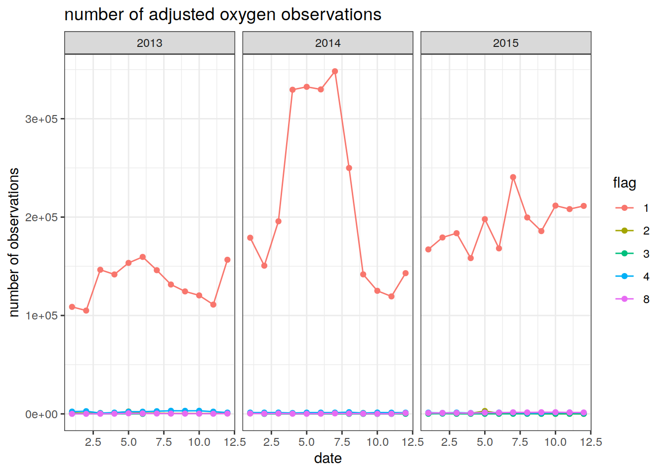
| Version | Author | Date |
|---|---|---|
| 4840e49 | pasqualina-vonlanthendinenna | 2021-10-12 |
pH
ph = data.frame(bgc_merge$longitude, bgc_merge$latitude, bgc_merge$date, bgc_merge$ph_in_situ_total_adjusted, bgc_merge$ph_in_situ_total_adjusted_qc)
# extract the variables from the combined data/metadata frame

colnames(ph) = c('longitude','latitude','date', 'ph_in_situ_total', 'flag')
# rename columns

ph$date.simple = as.Date(ph$date)
ph$time = format(ph$date, '%H:%M:%S') # separate date and time into two separate columns

ph = ph %>%
  mutate(year = year(date.simple),
         month = month(date.simple),
         day = day(date.simple),
         cycle = bgc_merge$cycle_number,
         float_ID = bgc_merge$float_serial_no,
         profile_flag = bgc_merge$profile_ph_in_situ_total_qc) # separate year, month and day, and add cycle number, float ID and profile qc flag

ph.no.na = ph %>%
  filter(!is.na(ph_in_situ_total)) # remove NA values

num_obs_ph = ph.no.na %>%
  group_by(year, month, flag) %>%
  summarise(Count = n())   # count the number of observations per month
`summarise()` has grouped output by 'year', 'month'. You can override using the `.groups` argument.We can then plot the number of pH observations in a timeseries. Different lines are plotted for different quality control flags
ggplot(num_obs_ph, aes(x = month, y = Count, group = flag, col = flag)) +
  geom_line() +
  geom_point() +
  facet_wrap(~year) +
  labs(title = 'number of adjusted pH observations',
       y = 'number of observations',
       x = 'date') +
  theme_bw()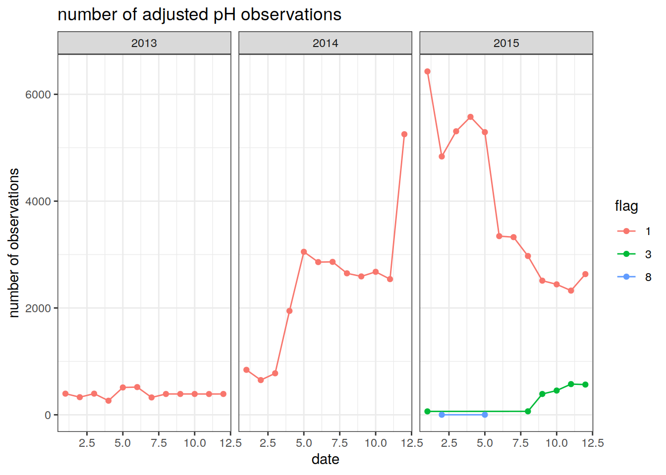
| Version | Author | Date |
|---|---|---|
| 4840e49 | pasqualina-vonlanthendinenna | 2021-10-12 |
Nitrate
nitrate = data.frame(bgc_merge$longitude, bgc_merge$latitude, bgc_merge$date, bgc_merge$nitrate_adjusted, bgc_merge$nitrate_adjusted_qc) # extract nitrate from the combined data/metadata dataframe

colnames(nitrate) = c('longitude','latitude', 'date', 'nitrate_adjusted', 'flag')
# rename columns

nitrate$date.simple = as.Date(nitrate$date)
nitrate$time = format(nitrate$date, '%H:%M:%S') # separate the date into date and time columns

nitrate = nitrate %>%
  mutate(year = year(date.simple),
         month = month(date.simple),
         day = day(date.simple),
         cycle = bgc_merge$cycle_number,
         float_ID = bgc_merge$float_serial_no,
         profile_flag = bgc_merge$profile_nitrate_qc) # separate year, month, and day, and add cycle number, float ID, and the profile qc flag

nitrate.no.na = nitrate %>%
  filter(!is.na(nitrate_adjusted)) # remove NA values

num_obs_nitrate = nitrate.no.na %>%
  group_by(year, month, flag) %>%
  summarise(Count = n())   # count the number of nitrate observations per month
`summarise()` has grouped output by 'year', 'month'. You can override using the `.groups` argument.Plot the number of nitrate observations per month as a timeseries. Different lines are plotted for different qc flags
ggplot(num_obs_nitrate, aes(x = month, y = Count, group = flag, col = flag))+
  geom_line()+
  geom_point()+
  facet_wrap(~ year)+
  labs(title = 'number of adjusted nitrate observations',
       y = 'number of observations',
       x = 'date') +
  theme_bw()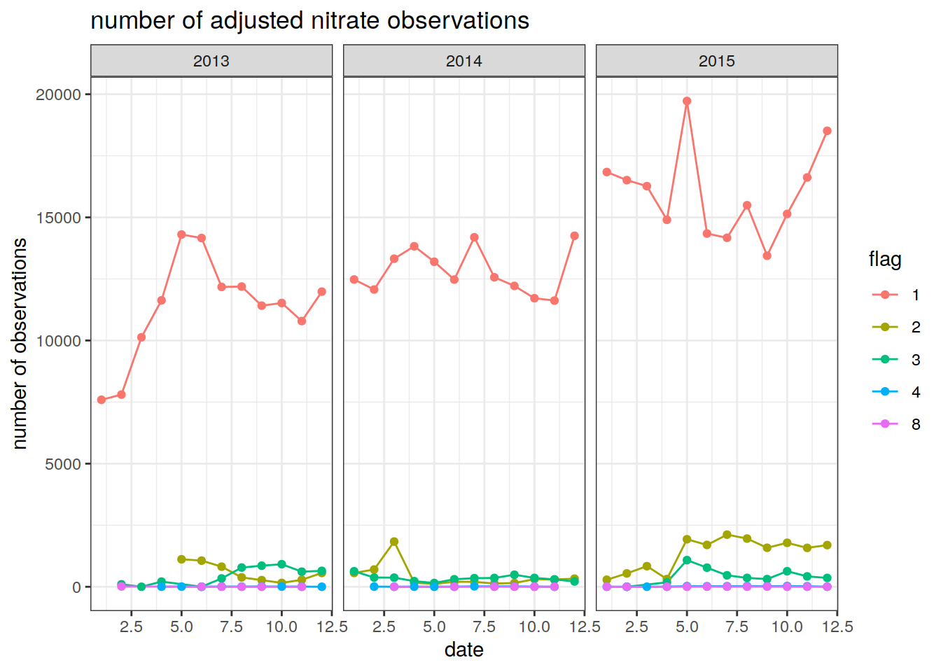
| Version | Author | Date |
|---|---|---|
| 4840e49 | pasqualina-vonlanthendinenna | 2021-10-12 |
All BGC variables
We can count the number of observations for which all three BGC variables exist. (QC flags cannot be included since they are specific to one variable)
# create a dataframe which contains all three variables, with longitude, latitude, date, cycle number and float ID
bgc_co_located = data.frame(bgc_merge$longitude, bgc_merge$latitude,
                            bgc_merge$date,
                            bgc_merge$cycle_number,
                            bgc_merge$float_serial_no,
                            bgc_merge$doxy_adjusted,
                            bgc_merge$ph_in_situ_total_adjusted,
                            bgc_merge$nitrate_adjusted)

colnames(bgc_co_located) = c('longitude', 'latitude',
                             'date',
                             'cycle',
                             'float_ID',
                             'doxy_adjusted',
                             'ph_in_situ_total_adjusted',
                             'nitrate_adjusted') # rename the columns

bgc_co_located = bgc_co_located %>%     # change the date and time format
  mutate(date.simple = as.Date(date),
         time = format(date, '%H:%M:%S'),
         year = year(date.simple),
         month = month(date.simple),
         day = day(date.simple))

bgc_co_located.no.na = bgc_co_located %>%  # remove NA values for each variable
  filter(!is.na(doxy_adjusted)) %>%
  filter(!is.na(ph_in_situ_total_adjusted)) %>%
  filter(!is.na(nitrate_adjusted))
# removes rows of pH and nitrate for which there is no oxygen, rows of oxygen and nitrate for which there is no pH, and rows of oxygen and pH for which there is no nitrate

# count the number of observations left for each year and month
num_obs_bgc = bgc_co_located.no.na %>%
  group_by(year, month) %>%
  summarise(Count = n())
`summarise()` has grouped output by 'year'. You can override using the `.groups` argument.We can then plot the evolution over time of the number of BGC observations containing all three variables
ggplot(num_obs_bgc, aes(x = month, y = Count))+
  geom_line()+
  geom_point()+
  facet_wrap(~ year)+
  labs(title = 'number of adjusted BGC observations',
       y = 'number of observations',
       x = 'date') +
  theme_bw()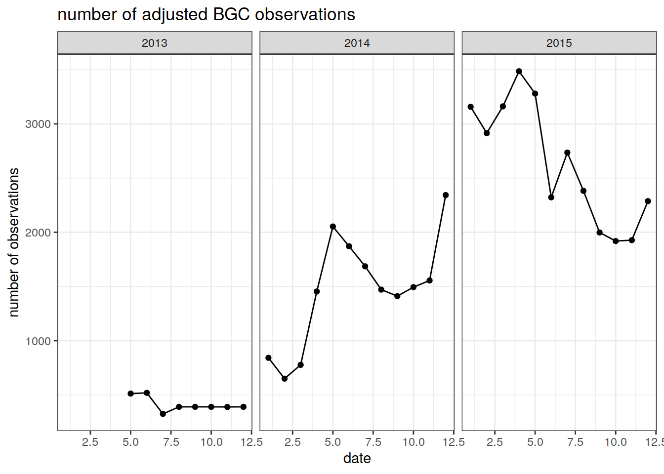
| Version | Author | Date |
|---|---|---|
| 795b5ad | pasqualina-vonlanthendinenna | 2021-10-13 |
NUMBER OF PROFILES
Using the dataframes created above for oxygen, pH, and nitrate, we can also look at the evolution of the number of profiles over time for each variable. (One profile has multiple depth levels, between 0-2000 m)
Oxygen
prof_oxy = oxy.no.na %>%
  group_by(float_ID, cycle, profile_flag, year, month) %>%
  summarise(num_obs = n())  # count the number of oxygen observations for each float and cycle
`summarise()` has grouped output by 'float_ID', 'cycle', 'profile_flag', 'year'. You can override using the `.groups` argument.num_prof_oxy = prof_oxy %>%
group_by(year, month, profile_flag) %>%
summarise(count_prof = n()) # count the number of 1s (profiles)`summarise()` has grouped output by 'year', 'month'. You can override using the `.groups` argument.Plot the evolution of the number of oxygen profiles over time
ggplot(num_prof_oxy,
       aes(
         x = month,
         y = count_prof,
         group = profile_flag,
         col = profile_flag
       )) +
  geom_line() +
  geom_point() +
  facet_wrap( ~ year, ncol = 3) +
  labs(title = 'number of oxygen profiles',
       y = 'number of profiles',
       x = 'month') +
  theme_bw()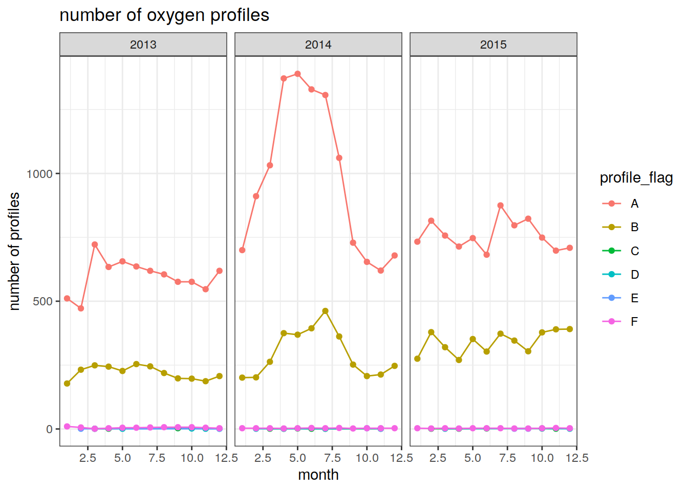
| Version | Author | Date |
|---|---|---|
| 4840e49 | pasqualina-vonlanthendinenna | 2021-10-12 |
pH
prof_ph = ph.no.na %>%
  group_by(float_ID, cycle, profile_flag, year, month) %>%
  summarise(num_obs = n()) # count the number of ph observations by float and cycle
`summarise()` has grouped output by 'float_ID', 'cycle', 'profile_flag', 'year'. You can override using the `.groups` argument.prof_ph = prof_ph %>%
mutate(prof = rep(1, length(cycle))) # repeat a vector of 1s over the length of the cycles (one cycle corresponds to one pH profile)
num_prof_ph = prof_ph %>%
group_by(year, month, profile_flag) %>%
summarise(count_prof = n()) # count the number of 1s (profiles)`summarise()` has grouped output by 'year', 'month'. You can override using the `.groups` argument.Plot the number of pH profiles over time
ggplot(num_prof_ph, aes(x = month, y = count_prof, group = profile_flag, col = profile_flag)) +
  geom_line() +
  geom_point() +
  facet_wrap(~ year, ncol = 3) +
  labs(title = 'number of pH profiles',
       y = 'number of profiles',
       x = 'month') +
  theme_bw()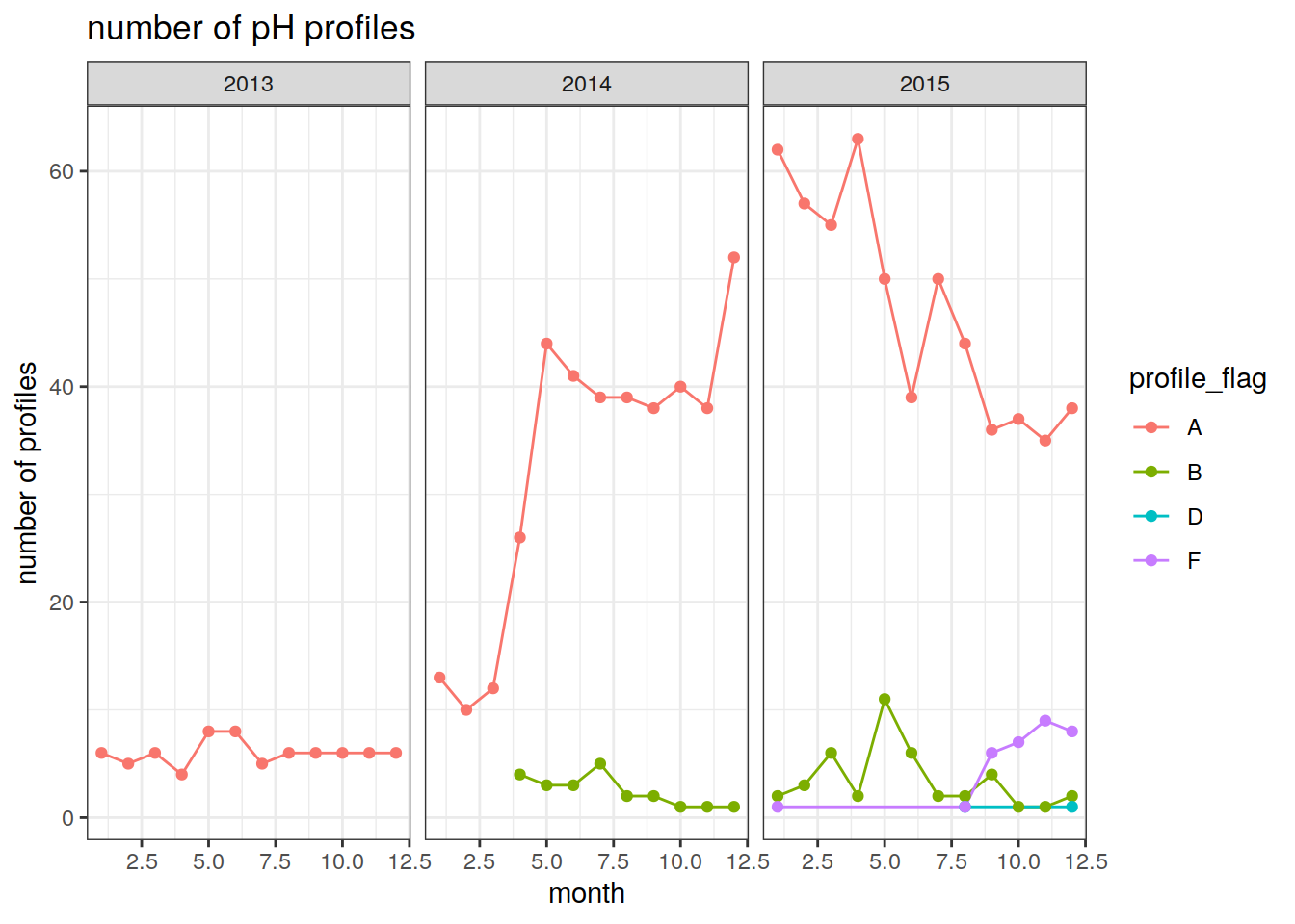
| Version | Author | Date |
|---|---|---|
| 4840e49 | pasqualina-vonlanthendinenna | 2021-10-12 |
Nitrate
prof_nitrate = nitrate.no.na %>%
  group_by(float_ID, cycle, profile_flag, year, month) %>%
  summarise(num_obs = n()) # count the number of nitrate observations by float and cycle
`summarise()` has grouped output by 'float_ID', 'cycle', 'profile_flag', 'year'. You can override using the `.groups` argument.prof_nitrate = prof_nitrate %>%
mutate(prof = rep(1, length(cycle))) # repeat a vector of 1s over the length of cycle numbers (one cycle is one profile)
num_prof_nitrate = prof_nitrate %>%
group_by(year, month, profile_flag) %>%
summarise(count_prof = n()) # count the number of 1s (profiles)`summarise()` has grouped output by 'year', 'month'. You can override using the `.groups` argument.Plot the number of nitrate profiles over time
ggplot(num_prof_nitrate, aes(x = month, y = count_prof, group = profile_flag, col = profile_flag)) +
  geom_line() +
  geom_point() +
  facet_wrap(~ year, ncol = 3) +
  labs(title = 'number of nitrate profiles',
       y = 'number of profiles',
       x = 'month') +
  theme_bw()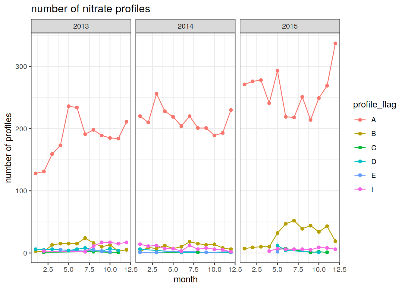
| Version | Author | Date |
|---|---|---|
| 4840e49 | pasqualina-vonlanthendinenna | 2021-10-12 |
All BGC variables
We can count the number of profiles which contain all three variables. (Profile QC flags cannot be included since they are specific to one variable)
# count the number of profiles for which all three variables exist
prof_bgc = bgc_co_located.no.na %>%
  group_by(float_ID, cycle, year, month) %>%
  summarise(num_obs = n()) # count the number of observations by float and cycle number
`summarise()` has grouped output by 'float_ID', 'cycle', 'year'. You can override using the `.groups` argument.prof_bgc = prof_bgc %>%
mutate(prof = rep(1, length(cycle))) # repeat a vector of 1s over the number of cycles
num_prof_bgc = prof_bgc %>%
group_by(year, month) %>%
summarise(count_prof = n()) # count the number of 1s `summarise()` has grouped output by 'year'. You can override using the `.groups` argument.Plot the number of BGC profiles for which all three variables exist over time
ggplot(num_prof_bgc, aes(x = month, y = count_prof)) +
  geom_line() +
  geom_point() +
  facet_wrap(~ year) +
  labs(title = 'number of BGC profiles',
       y = 'number of profiles',
       x = 'month') +
  theme_bw()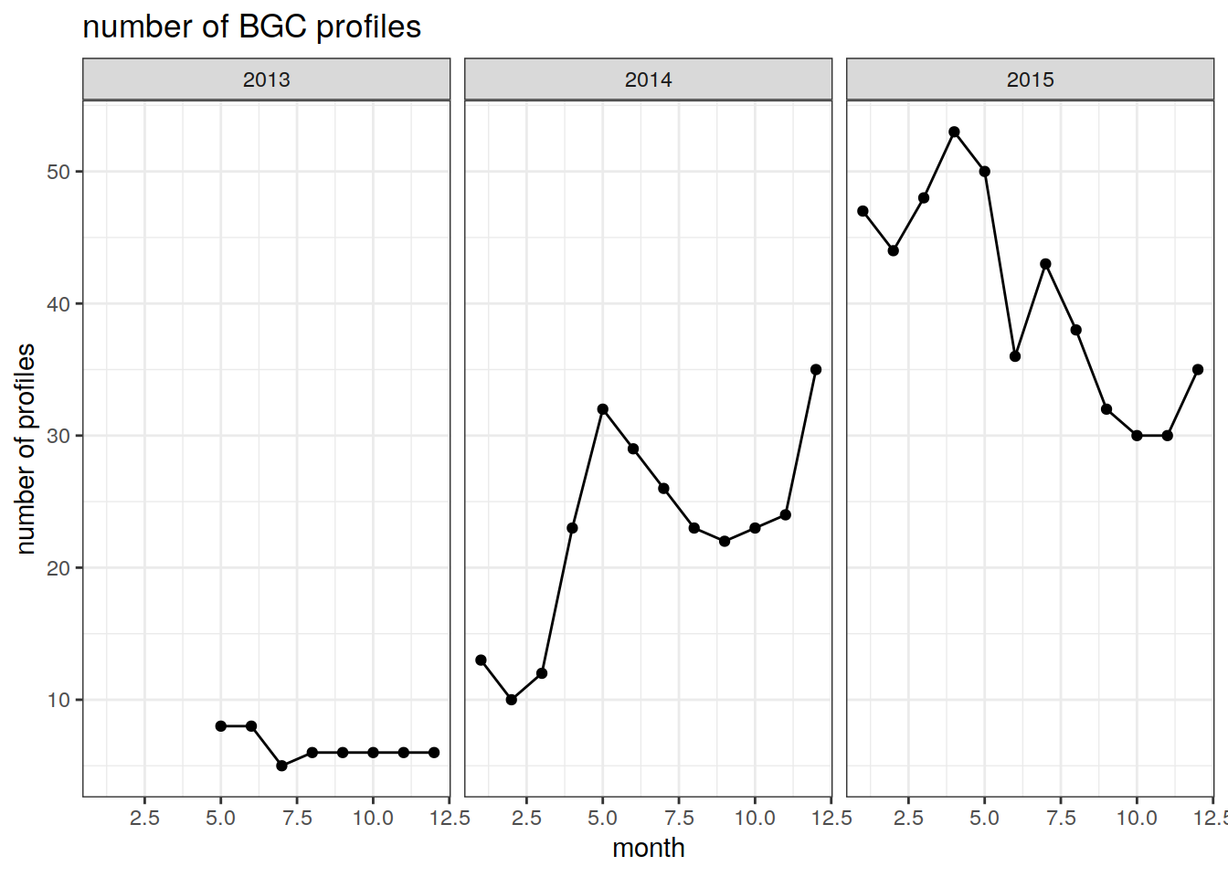
| Version | Author | Date |
|---|---|---|
| 5331669 | pasqualina-vonlanthendinenna | 2021-10-13 |
Number of profiles revised
bgc_profile_counts <- bgc_metadata %>%
  select(platform_number, cycle_number, date,
         profile_doxy_qc, profile_ph_in_situ_total_qc, profile_nitrate_qc) %>%
  pivot_longer(cols = profile_doxy_qc:profile_nitrate_qc,
               names_to = "profile_qc",
               values_to = "flag",
               names_prefix = "profile_") %>%
  mutate(year = year(date),
         month = month(date)) %>%
  count(year, month, profile_qc, flag) %>%
  filter(!is.na(flag),
         flag != "")
Plot the evolution of the number of profiles over time
bgc_profile_counts %>%
  ggplot(aes(x = month, y = n, col = flag)) +
  geom_line() +
  geom_point() +
  facet_grid(profile_qc ~ year,
             scales = "free_y") +
  theme_bw()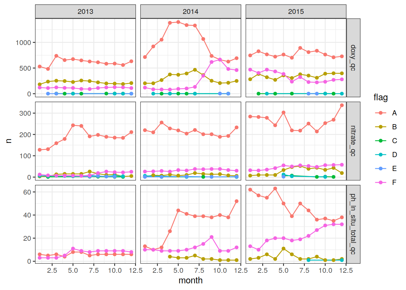
bgc_profile_counts %>%
  group_split(profile_qc) %>%
  map(
    ~ ggplot(data = .x,
             aes(
               x = month, y = n, col = flag
             )) +
      geom_line() +
      geom_point() +
      facet_grid(. ~ year,
                 scales = "free_y") +
      labs(title = paste("Parameter: ", unique(.x$profile_qc))) +
      theme_bw()
  )
[[1]]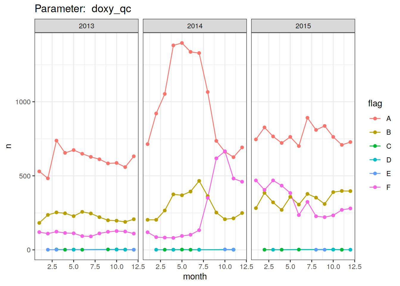
[[2]]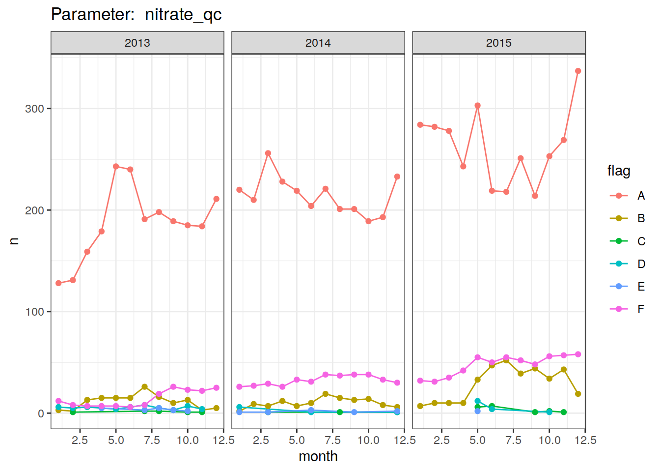
[[3]]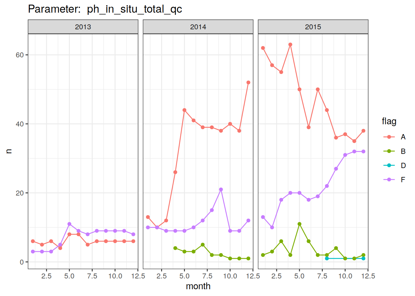
bgc_profile_counts_total_A <- bgc_metadata %>%
  select(platform_number, cycle_number, date,
         profile_doxy_qc, profile_ph_in_situ_total_qc, profile_nitrate_qc) %>%
  pivot_longer(cols = profile_doxy_qc:profile_nitrate_qc,
               names_to = "profile_qc",
               values_to = "flag",
               names_prefix = "profile_") %>%
  mutate(year = year(date),
         month = month(date)) %>%
  filter(flag == "A") %>%
  distinct(platform_number, cycle_number, year, month) %>%
  count(year, month)
bgc_profile_counts_total_A %>%
ggplot(aes(x = month, y = n)) +
geom_line() +
geom_point() +
facet_grid(. ~ year,
scales = "free_y") +
scale_x_continuous(breaks = seq(1,12,2)) +
theme_bw()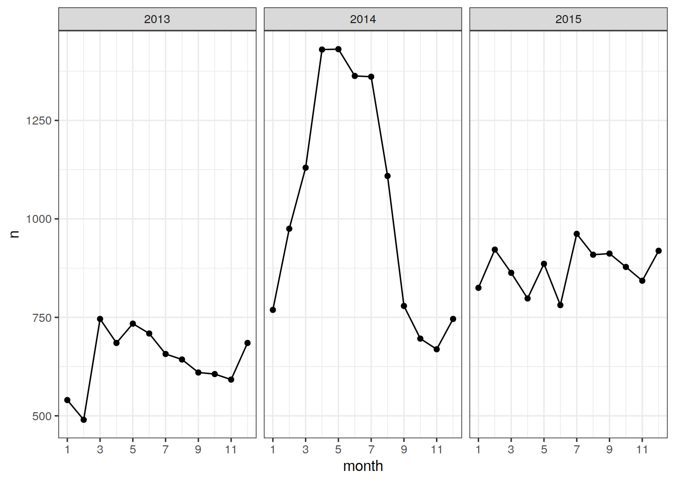
sessionInfo()R version 4.0.3 (2020-10-10)
Platform: x86_64-pc-linux-gnu (64-bit)
Running under: openSUSE Leap 15.2
Matrix products: default
BLAS: /usr/local/R-4.0.3/lib64/R/lib/libRblas.so
LAPACK: /usr/local/R-4.0.3/lib64/R/lib/libRlapack.so
locale:
[1] LC_CTYPE=en_US.UTF-8 LC_NUMERIC=C
[3] LC_TIME=en_US.UTF-8 LC_COLLATE=en_US.UTF-8
[5] LC_MONETARY=en_US.UTF-8 LC_MESSAGES=en_US.UTF-8
[7] LC_PAPER=en_US.UTF-8 LC_NAME=C
[9] LC_ADDRESS=C LC_TELEPHONE=C
[11] LC_MEASUREMENT=en_US.UTF-8 LC_IDENTIFICATION=C
attached base packages:
[1] stats graphics grDevices utils datasets methods base
other attached packages:
[1] lubridate_1.7.9 argodata_0.0.0.9000 forcats_0.5.0
[4] stringr_1.4.0 dplyr_1.0.5 purrr_0.3.4
[7] readr_1.4.0 tidyr_1.1.3 tibble_3.1.3
[10] ggplot2_3.3.5 tidyverse_1.3.0 workflowr_1.6.2
loaded via a namespace (and not attached):
[1] Rcpp_1.0.5 assertthat_0.2.1 rprojroot_2.0.2 digest_0.6.27
[5] utf8_1.1.4 R6_2.5.0 cellranger_1.1.0 backports_1.1.10
[9] reprex_0.3.0 evaluate_0.14 highr_0.8 httr_1.4.2
[13] pillar_1.6.2 rlang_0.4.11 readxl_1.3.1 rstudioapi_0.13
[17] whisker_0.4 jquerylib_0.1.4 blob_1.2.1 rmarkdown_2.10
[21] labeling_0.4.2 munsell_0.5.0 broom_0.7.9 compiler_4.0.3
[25] httpuv_1.5.4 modelr_0.1.8 xfun_0.25 pkgconfig_2.0.3
[29] htmltools_0.5.1.1 tidyselect_1.1.0 fansi_0.4.1 crayon_1.3.4
[33] dbplyr_1.4.4 withr_2.3.0 later_1.2.0 grid_4.0.3
[37] jsonlite_1.7.1 gtable_0.3.0 lifecycle_1.0.0 DBI_1.1.0
[41] git2r_0.27.1 magrittr_1.5 scales_1.1.1 cli_3.0.1
[45] stringi_1.5.3 farver_2.0.3 fs_1.5.0 promises_1.1.1
[49] xml2_1.3.2 bslib_0.2.5.1 ellipsis_0.3.2 generics_0.1.0
[53] vctrs_0.3.8 tools_4.0.3 glue_1.4.2 RNetCDF_2.4-2
[57] hms_0.5.3 yaml_2.2.1 colorspace_2.0-2 rvest_0.3.6
[61] knitr_1.33 haven_2.3.1 sass_0.4.0