Map BGC Argo observations

workflowr

• Summary
• Checks
• Past versions

Last updated: 2021-10-19

Checks: 7 0

Knit directory: bgc_argo_r_argodata/

This reproducible R Markdown analysis was created with workflowr (version 1.6.2). The Checks tab describes the reproducibility checks that were applied when the results were created. The Past versions tab lists the development history.

---

R Markdown file: up-to-date

Great! Since the R Markdown file has been committed to the Git repository, you know the exact version of the code that produced these results.

Environment: empty

Great job! The global environment was empty. Objects defined in the global environment can affect the analysis in your R Markdown file in unknown ways. For reproduciblity it’s best to always run the code in an empty environment.

Seed: set.seed(20211008)

The command set.seed(20211008) was run prior to running the code in the R Markdown file. Setting a seed ensures that any results that rely on randomness, e.g. subsampling or permutations, are reproducible.

Session information: recorded

Great job! Recording the operating system, R version, and package versions is critical for reproducibility.

Cache: none

Nice! There were no cached chunks for this analysis, so you can be confident that you successfully produced the results during this run.

File paths: relative

Great job! Using relative paths to the files within your workflowr project makes it easier to run your code on other machines.

Repository version: f460b9a

Great! You are using Git for version control. Tracking code development and connecting the code version to the results is critical for reproducibility.

The results in this page were generated with repository version f460b9a. See the Past versions tab to see a history of the changes made to the R Markdown and HTML files.

Note that you need to be careful to ensure that all relevant files for the analysis have been committed to Git prior to generating the results (you can use wflow_publish or wflow_git_commit). workflowr only checks the R Markdown file, but you know if there are other scripts or data files that it depends on. Below is the status of the Git repository when the results were generated:

Ignored files:
    Ignored:    .Rhistory
    Ignored:    .Rproj.user/

Unstaged changes:
    Modified:   code/Workflowr_project_managment.R

Note that any generated files, e.g. HTML, png, CSS, etc., are not included in this status report because it is ok for generated content to have uncommitted changes.

---

These are the previous versions of the repository in which changes were made to the R Markdown (analysis/map_observations.Rmd) and HTML (docs/map_observations.html) files. If you’ve configured a remote Git repository (see ?wflow_git_remote), click on the hyperlinks in the table below to view the files as they were in that past version.

File	Version	Author	Date	Message
Rmd	f460b9a	jens-daniel-mueller	2021-10-19	code review jens
html	830edff	pasqualina-vonlanthendinenna	2021-10-15	Build site.
Rmd	b19b3cf	pasqualina-vonlanthendinenna	2021-10-15	fixed subtitle
html	2420353	pasqualina-vonlanthendinenna	2021-10-15	Build site.
Rmd	c8c1bd5	pasqualina-vonlanthendinenna	2021-10-15	changed fontsize in mapping titles
html	2979534	pasqualina-vonlanthendinenna	2021-10-15	Build site.
Rmd	895351d	pasqualina-vonlanthendinenna	2021-10-15	changed fontsize in mapping titles
html	83724a0	pasqualina-vonlanthendinenna	2021-10-14	Build site.
Rmd	6a2a266	pasqualina-vonlanthendinenna	2021-10-14	added map observations page

---

Task

Map the location of oxygen, pH, and nitrate observations recorded by BGC-Argo floats

library(tidyverse, quiet = TRUE)

── Attaching packages ─────────────────────────────────────── tidyverse 1.3.0 ──

✓ ggplot2 3.3.5     ✓ purrr   0.3.4
✓ tibble  3.1.3     ✓ dplyr   1.0.5
✓ tidyr   1.1.3     ✓ stringr 1.4.0
✓ readr   1.4.0     ✓ forcats 0.5.0

── Conflicts ────────────────────────────────────────── tidyverse_conflicts() ──
x dplyr::filter() masks stats::filter()
x dplyr::lag()    masks stats::lag()

library(argodata, quiet = TRUE)
library(ggplot2, quiet = TRUE)
library(lubridate, quiet = TRUE)

Attaching package: 'lubridate'

The following objects are masked from 'package:base':

    date, intersect, setdiff, union

library(sf, quiet = TRUE)

Linking to GEOS 3.6.2, GDAL 3.0.4, PROJ 7.0.0

library(rnaturalearth, quiet = TRUE)
library(rnaturalearthdata, quiet = TRUE)
# load in coastline data (uses sf and rnaturalearthdata packages)
world = ne_coastline(scale = 'medium', returnclass = 'sf')

Load data

Read the files created in loading_data.html:

path_argo_preprocessed <- paste0(path_argo, "/preprocessed_bgc_data")

bgc_subset <-
  read_rds(file = paste0(path_argo_preprocessed, "/bgc_subset.rds"))

bgc_metadata <-
  read_rds(file = paste0(path_argo_preprocessed, "/bgc_metadata.rds"))

bgc_data <-
  read_rds(file = paste0(path_argo_preprocessed, "/bgc_data.rds"))

bgc_merge <-
  read_rds(file = paste0(path_argo_preprocessed, "/bgc_merge.rds"))

# Set the cache directory using argo_set_cache_dir():
argo_set_cache_dir('/nfs/kryo/work/updata/bgc_argo_r_argodata')
argo_update_global(max_global_cache_age = Inf)
argo_update_data(max_data_cache_age = Inf)

bgc_subset = argo_global_synthetic_prof() %>%
  argo_filter_data_mode(data_mode = 'delayed') %>%
  argo_filter_date(date_min = '2013-01-01',
                   date_max = '2015-12-31') # download the indexes of synthetic files of delayed-mode data (BGC and core argo data)

# check the dates 
# max(bgc_subset$date, na.rm = TRUE)
# min(bgc_subset$date, na.rm = TRUE)


bgc_data = argo_prof_levels(bgc_subset, vars = c('PRES_ADJUSTED','PRES_ADJUSTED_QC',
                                                 'PSAL_ADJUSTED', 'PSAL_ADJUSTED_QC',
                                                 'TEMP_ADJUSTED','TEMP_ADJUSTED_QC',
                                                 'DOXY_ADJUSTED', 'DOXY_ADJUSTED_QC',
                                                 'NITRATE_ADJUSTED', 'NITRATE_ADJUSTED_QC',
                                                 'PH_IN_SITU_TOTAL_ADJUSTED', 'PH_IN_SITU_TOTAL_ADJUSTED_QC'), quiet = TRUE)
# read in the profiles (takes a while)

bgc_metadata = argo_prof_prof(bgc_subset)  # load in the corresponding metadata

bgc_merge = left_join(bgc_data, bgc_metadata, by = c('file', 'n_prof'))
# joins the metadata to the data and creates one data frame

MAP OF OBSERVATIONS

Create separate dataframes for each variable, with longitude, latitude, date, value, cycle number, and float ID

Oxygen

oxy = data.frame(bgc_merge$longitude, bgc_merge$latitude, bgc_merge$date,
                 bgc_merge$doxy_adjusted) # add longitude, latitude, date and oxygen to the dataframe 
colnames(oxy) = c('longitude','latitude','date', 'doxy_adjusted') # rename columns 

oxy = oxy %>%
  mutate(date.simple = as.Date(date),    # create one date and one time column
         time = format(date, '%H:%M:%S'),
         cycle = bgc_merge$cycle_number, # add cycle number and float ID 
         float_ID = bgc_merge$float_serial_no)

oxy.no.na = oxy %>%
  filter(!is.na(doxy_adjusted)) # remove the NA values

location_obs_oxy = oxy.no.na %>%
  group_by(round(longitude, digits = 0), round(latitude, digits = 0)) %>% 
  summarise(Count = n()) # count the number of data points per longitude/latitude pair, rounded to the nearest integer 

`summarise()` has grouped output by 'round(longitude, digits = 0)'. You can override using the `.groups` argument.

colnames(location_obs_oxy) = c('longitude', 'latitude', 'Count') # rename columns

Map the location of the oxygen observations

ggplot() +
  geom_tile(data = location_obs_oxy, aes(x = longitude, y = latitude, fill = Count))+
  geom_sf(data = world, fill = 'grey')+
  scale_fill_gradientn(colors = rev(rainbow(10)))+
  theme_bw()+
  labs(x = 'longitude', y = 'latitude', fill = 'number of obs',
       title = 'location of delayed-mode adjusted oxygen observations')

Warning: Removed 1 rows containing missing values (geom_tile).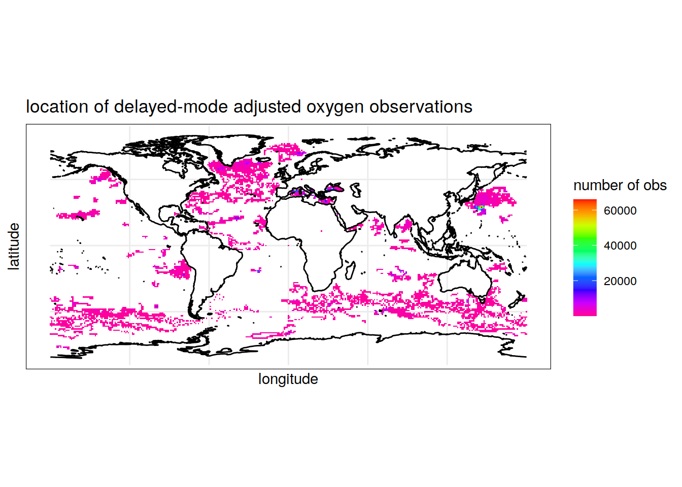

Past versions of map_oxygen_observations-1.png

Version	Author	Date
83724a0	pasqualina-vonlanthendinenna	2021-10-14

pH

ph = data.frame(bgc_merge$longitude, bgc_merge$latitude, bgc_merge$date,
                bgc_merge$ph_in_situ_total_adjusted) # add longitude, latitude, date, and pH to a dataframe 

colnames(ph) = c('longitude','latitude','date', 'ph_in_situ_total') #rename columns

ph = ph %>%
  mutate(date.simple = as.Date(date),  # create one date and one time columns
         time = format(date, '%H:%M:%S'),
         cycle = bgc_merge$cycle_number,  # add cycle number and float ID
         float_ID = bgc_merge$float_serial_no)

ph.no.na = ph %>%
  filter(!is.na(ph_in_situ_total)) # remove NA values 

location_obs_ph = ph.no.na %>%
  group_by(round(longitude, digits = 0), round(latitude, digits = 0)) %>%
  summarise(Count = n()) # count the number of pH observations for each longitude/latitude pair rounded to the nearest integer 

`summarise()` has grouped output by 'round(longitude, digits = 0)'. You can override using the `.groups` argument.

colnames(location_obs_ph) = c('longitude', 'latitude', 'Count') # rename columns 

Map the location of pH observations

ggplot() +
  geom_sf(data = world, fill = 'grey')+
  geom_tile(data = location_obs_ph, aes(x = longitude, y = latitude, fill = Count))+
  scale_fill_gradientn(colors = rev(rainbow(10)))+
  theme_bw()+
  labs(x = 'longitude', y = 'latitude', fill = 'number of obs',
       title = 'location of delayed-mode adjusted pH observations')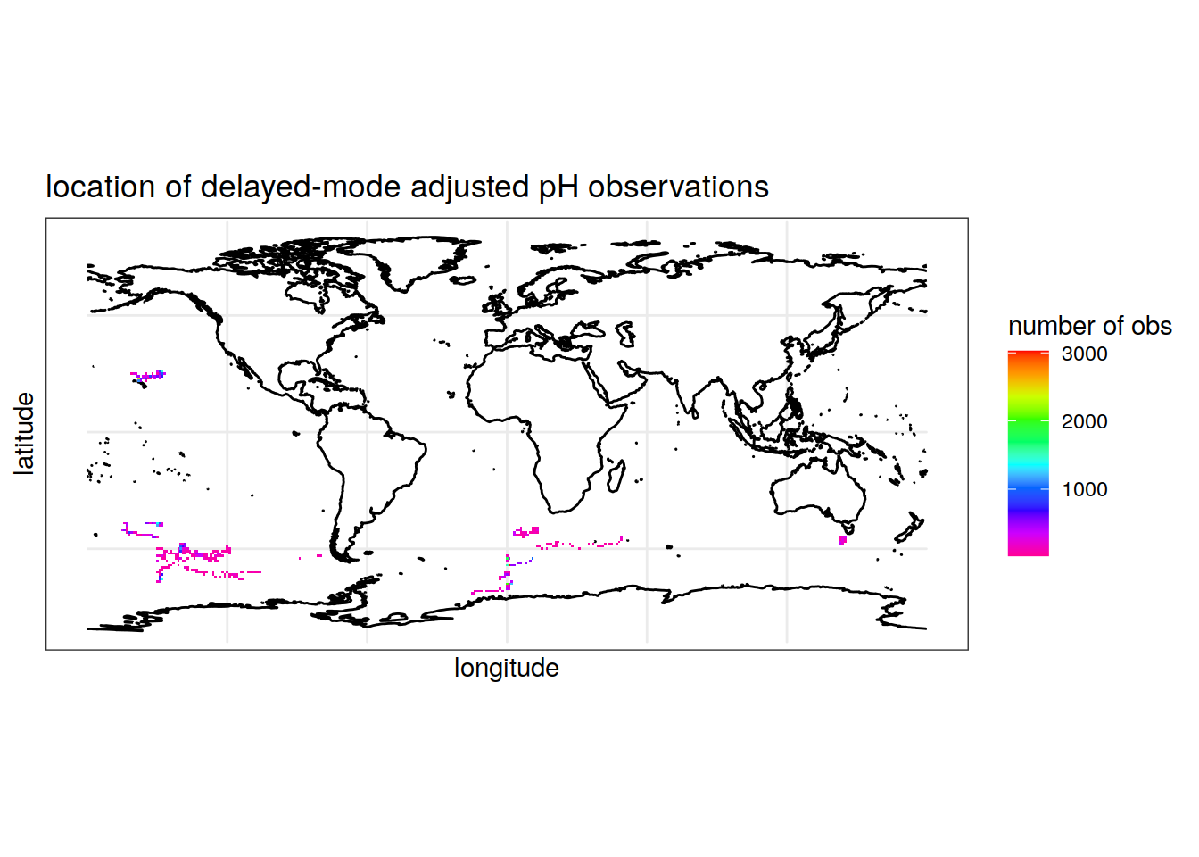

Past versions of map_pH_observations-1.png

Version	Author	Date
83724a0	pasqualina-vonlanthendinenna	2021-10-14

Nitrate

nitrate = data.frame(bgc_merge$longitude, bgc_merge$latitude, bgc_merge$date,
                     bgc_merge$nitrate_adjusted) # create a dataframe with longitude, latitude, date, and nitrate values 

colnames(nitrate) = c('longitude','latitude', 'date', 'nitrate_adjusted') # rename columns

nitrate = nitrate %>%
  mutate(date.simple = as.Date(date),  # separate date and time into two columns 
         time = format(date, '%H:%M:%S'),
         cycle = bgc_merge$cycle_number,  # add cycle number and float ID 
         float_ID = bgc_merge$float_serial_no)

nitrate.no.na = nitrate %>%
  filter(!is.na(nitrate_adjusted)) # remove NA values 

location_obs_nitrate = nitrate.no.na %>%
  group_by(round(longitude, digits = 0), round(latitude, digits = 0)) %>%
  summarise(Count = n()) # count the number of nitrate observations for each longitude/latitude pair rounded to the nearest integer 

`summarise()` has grouped output by 'round(longitude, digits = 0)'. You can override using the `.groups` argument.

colnames(location_obs_nitrate) = c('longitude', 'latitude', 'Count') # rename columns 

Map the location of nitrate observations

ggplot() +
  geom_tile(data = location_obs_nitrate, aes(x = longitude, y = latitude, fill = Count))+
  geom_sf(data = world, fill = 'grey')+
  scale_fill_gradientn(colors = rev(rainbow(10)))+
  theme_bw()+
  labs(x = 'longitude', y = 'latitude', fill = 'number of obs',
       title = 'location of delayed-mode adjusted nitrate observations')

Warning: Removed 1 rows containing missing values (geom_tile).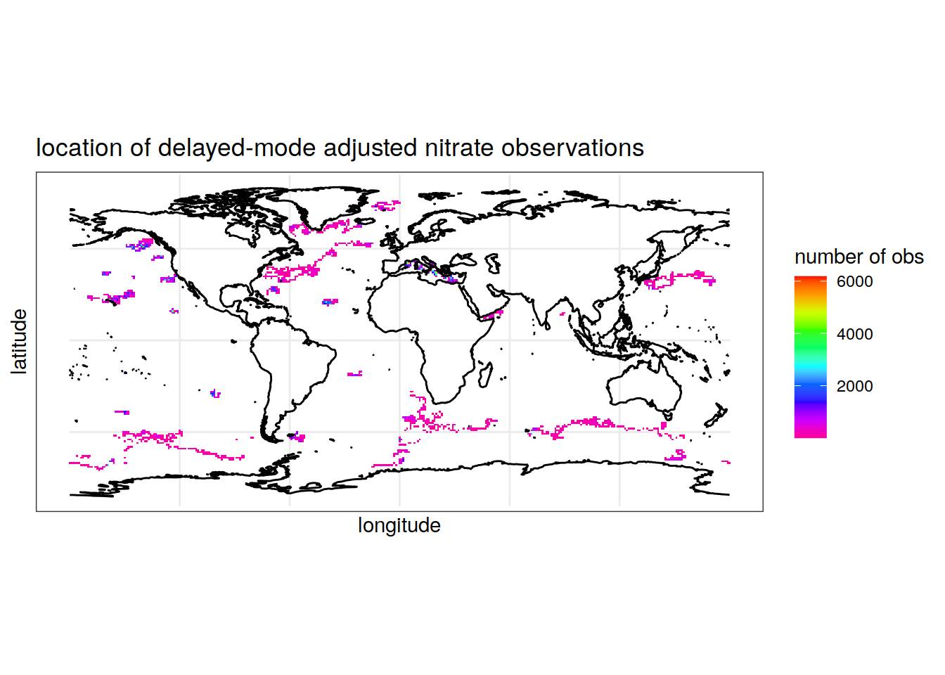

Past versions of map_nitrate_observations-1.png

Version	Author	Date
83724a0	pasqualina-vonlanthendinenna	2021-10-14

All BGC variables

Map the location of observations for which a measurement of all three variables exists

# create a dataframe which contains longitude, latitude, date, cycle number, float ID, and all three bgc variables 
bgc_co_located = data.frame(bgc_merge$longitude, bgc_merge$latitude,
                            bgc_merge$date,
                            bgc_merge$cycle_number,
                            bgc_merge$float_serial_no,
                            bgc_merge$doxy_adjusted,
                            bgc_merge$ph_in_situ_total_adjusted,
                            bgc_merge$nitrate_adjusted)

# rename columns:
colnames(bgc_co_located) = c('longitude', 'latitude',
                             'date',
                             'cycle',
                             'float_ID',
                             'doxy_adjusted',
                             'ph_in_situ_total_adjusted',
                             'nitrate_adjusted')

bgc_co_located = bgc_co_located %>%    # change the date and time format
  mutate(date.simple = as.Date(date),
         time = format(date, '%H:%M:%S'))

bgc_co_located.no.na = bgc_co_located %>%  # remove NA values for each variable
  filter(!is.na(doxy_adjusted)) %>%
  filter(!is.na(ph_in_situ_total_adjusted)) %>%
  filter(!is.na(nitrate_adjusted))

location_obs_bgc = bgc_co_located.no.na %>% 
  group_by(round(longitude, digits = 0), round(latitude, digits = 0)) %>%
  summarise(Count = n()) # count the number of observations for each longitude/latitude pair, rounded to the nearest integer

`summarise()` has grouped output by 'round(longitude, digits = 0)'. You can override using the `.groups` argument.

colnames(location_obs_bgc) = c('longitude', 'latitude', 'Count') # rename columns 

Map the locations of BGC observations

ggplot() +
  geom_tile(data = location_obs_bgc, aes(x = longitude, y = latitude, fill = Count))+
  geom_sf(data = world, fill = 'grey')+
  scale_fill_gradientn(colors = rev(rainbow(10)))+
  theme_bw()+
  labs(x = 'longitude', y = 'latitude', fill = 'number of obs',
       title = 'location of delayed-mode adjusted BGC observations (oxygen, pH, and nitrate)')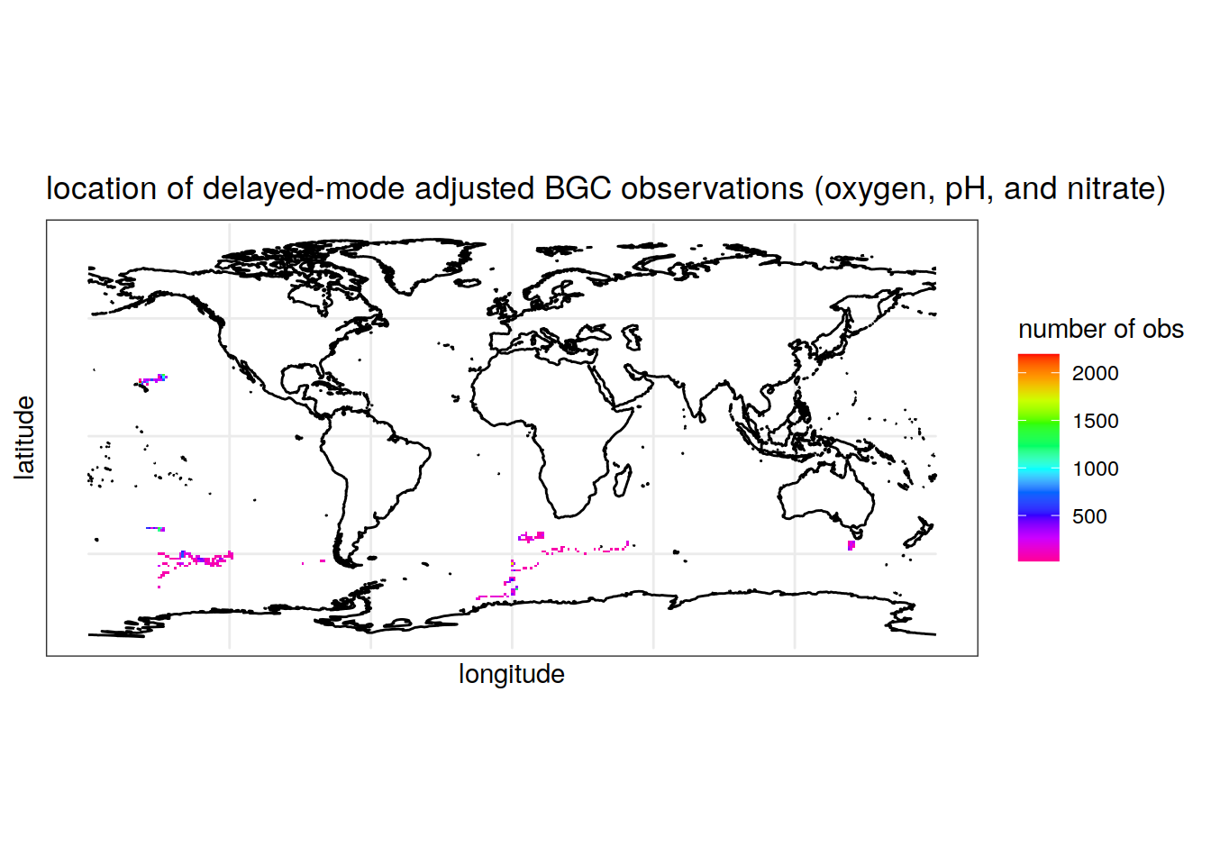

Past versions of map_bgc_observations-1.png

Version	Author	Date
83724a0	pasqualina-vonlanthendinenna	2021-10-14

MAP OF PROFILE LOCATIONS

Oxygen

# count the number of oxygen profiles
prof_oxy = oxy.no.na %>%
  group_by(float_ID, cycle, round(longitude, digits = 0), round(latitude, digits = 0)) %>%    
  summarise(num_obs = n())  # count the number of oxygen observations by float and cycle

`summarise()` has grouped output by 'float_ID', 'cycle', 'round(longitude, digits = 0)'. You can override using the `.groups` argument.

colnames(prof_oxy) = c('float_ID', 'cycle', 'longitude', 'latitude', 'num_obs') # rename columns

prof_oxy = prof_oxy %>%
  mutate(prof = rep(1, length(cycle))) # repeat a vector of 1s for each individual cycle 

location_prof_oxy = prof_oxy %>%
  group_by(round(longitude, digits = 0), round(latitude, digits = 0)) %>%
  summarise(count_prof = n())       # count the number of 1s (profiles) for each longitude/latitude pair, rounded to the nearest integer 

`summarise()` has grouped output by 'round(longitude, digits = 0)'. You can override using the `.groups` argument.

colnames(location_prof_oxy) = c('longitude', 'latitude', 'Count')

Map the location of oxygen profiles

ggplot() +
  geom_tile(data = location_prof_oxy, aes(x = longitude, y = latitude, fill = Count))+
  geom_sf(data = world, fill = 'grey')+
  scale_fill_gradientn(colors = rev(rainbow(10)))+
  theme_bw()+
  labs(x = 'longitude', y = 'latitude', fill = 'number of profiles',
       title = 'location of delayed-mode adjusted oxygen profiles')

Warning: Removed 1 rows containing missing values (geom_tile).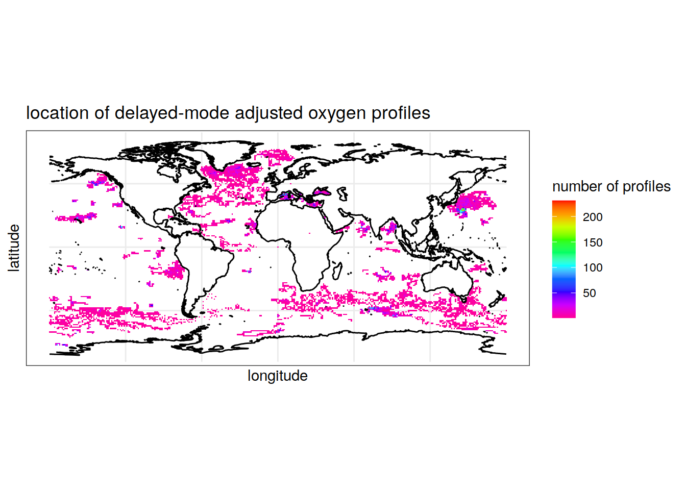

Past versions of map_oxygen_profiles-1.png

Version	Author	Date
83724a0	pasqualina-vonlanthendinenna	2021-10-14

pH

# count the number of pH profiles
prof_ph = ph.no.na %>%
  group_by(float_ID, cycle, round(longitude, digits = 0), round(latitude, digits = 0)) %>%    
  summarise(num_obs = n())  # count the number of ph observations by float and cycle

`summarise()` has grouped output by 'float_ID', 'cycle', 'round(longitude, digits = 0)'. You can override using the `.groups` argument.

colnames(prof_ph) = c('float_ID', 'cycle', 'longitude', 'latitude', 'num_obs') # rename columns

prof_ph = prof_ph %>%
  mutate(prof = rep(1, length(cycle))) # repeat a vector of 1s for each individual cycle 

location_prof_ph = prof_ph %>%
  group_by(round(longitude, digits = 0), round(latitude, digits = 0)) %>%
  summarise(count_prof = n())       # count the number of 1s (profiles) for each longitude/latitude pair, rounded to the nearest integer 

`summarise()` has grouped output by 'round(longitude, digits = 0)'. You can override using the `.groups` argument.

colnames(location_prof_ph) = c('longitude', 'latitude', 'Count') # rename columns 

Map the location of pH profiles

ggplot() +
  geom_tile(data = location_prof_ph, aes(x = longitude, y = latitude, fill = Count))+
  geom_sf(data = world, fill = 'grey')+
  scale_fill_gradientn(colors = rev(rainbow(10)))+
  theme_bw()+
  labs(x = 'longitude', y = 'latitude', fill = 'number of profiles',
       title = 'location of delayed-mode adjusted pH profiles')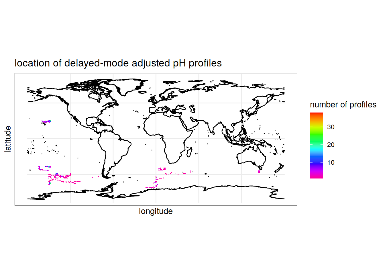

Past versions of map_pH_profiles-1.png

Version	Author	Date
83724a0	pasqualina-vonlanthendinenna	2021-10-14

Nitrate

# count the number of nitrate profiles
prof_nitrate = nitrate.no.na %>%
  group_by(float_ID, cycle, round(longitude, digits = 0), round(latitude, digits = 0)) %>%    
  summarise(num_obs = n())  # count the number of nitrate observations by float and cycle

`summarise()` has grouped output by 'float_ID', 'cycle', 'round(longitude, digits = 0)'. You can override using the `.groups` argument.

colnames(prof_nitrate) = c('float_ID', 'cycle', 'longitude', 'latitude', 'num_obs') # rename columns

prof_nitrate = prof_nitrate %>%
  mutate(prof = rep(1, length(cycle))) # repeat a vector of 1s for each individual cycle 

location_prof_nitrate = prof_nitrate %>%
  group_by(round(longitude, digits = 0), round(latitude, digits = 0)) %>%
  summarise(count_prof = n())       # count the number of 1s (profiles) for each longitude/latitude pair, rounded to the nearest integer 

`summarise()` has grouped output by 'round(longitude, digits = 0)'. You can override using the `.groups` argument.

colnames(location_prof_nitrate) = c('longitude', 'latitude', 'Count') # rename columns

Map the location of nitrate profiles

ggplot() +
  geom_tile(data = location_prof_nitrate, aes(x = longitude, y = latitude, fill = Count))+
  geom_sf(data = world, fill = 'grey')+
  scale_fill_gradientn(colors = rev(rainbow(10)))+
  theme_bw()+
  labs(x = 'longitude', y = 'latitude', fill = 'number of profiles',
       title = 'location of delayed-mode adjusted nitrate profiles')

Warning: Removed 1 rows containing missing values (geom_tile).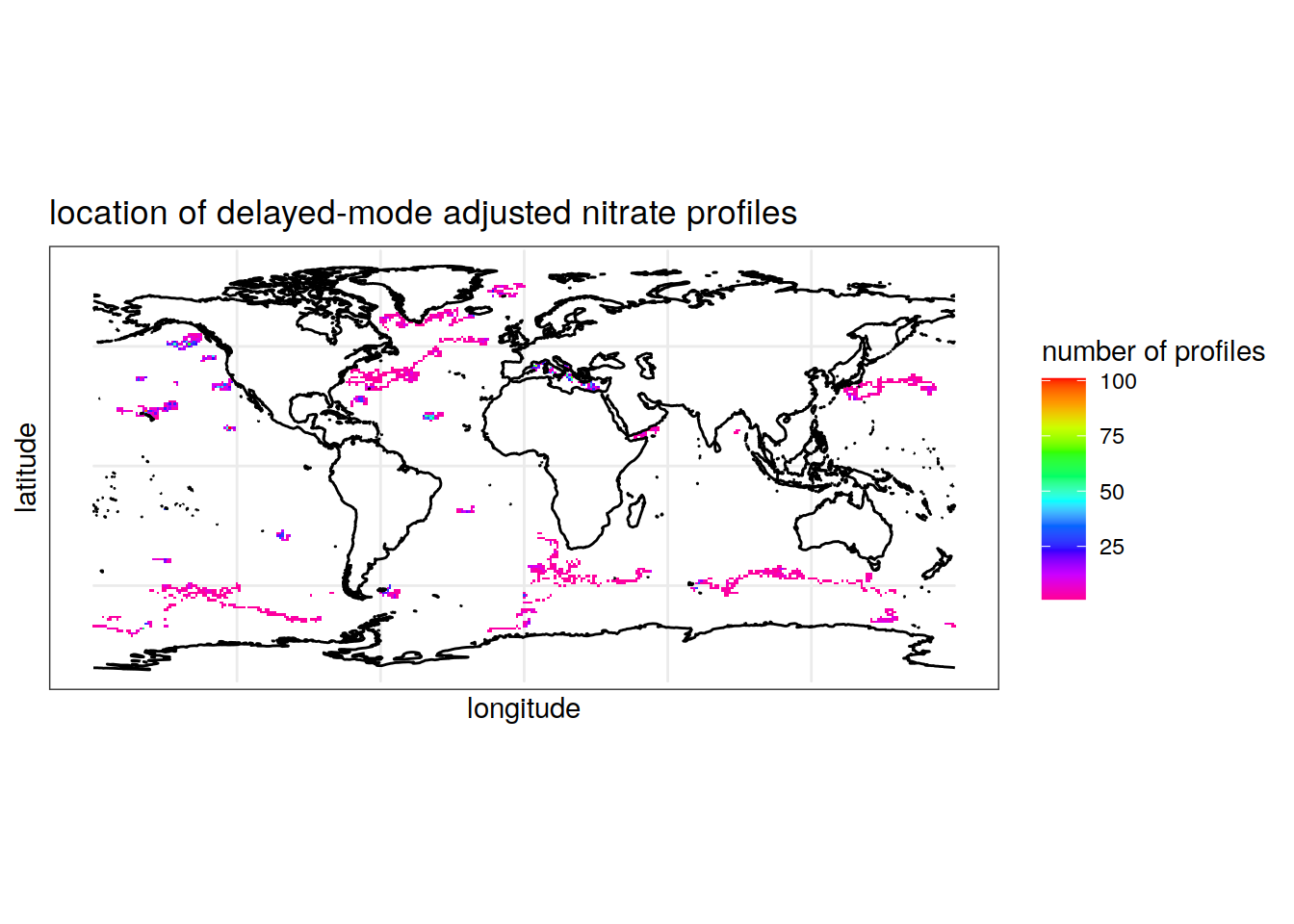

Past versions of map_nitrate_profiles-1.png

Version	Author	Date
83724a0	pasqualina-vonlanthendinenna	2021-10-14

All BGC variables

# count the number of bgc profiles
prof_bgc = bgc_co_located.no.na %>%
  group_by(float_ID, cycle, round(longitude, digits = 0), round(latitude, digits = 0)) %>%    
  summarise(num_obs = n())  # count the number of nitrate observations by float and cycle

`summarise()` has grouped output by 'float_ID', 'cycle', 'round(longitude, digits = 0)'. You can override using the `.groups` argument.

colnames(prof_bgc) = c('float_ID', 'cycle', 'longitude', 'latitude', 'num_obs') # rename columns

prof_bgc = prof_bgc %>%
  mutate(prof = rep(1, length(cycle))) # repeat a vector of 1s for each individual cycle 

location_prof_bgc = prof_bgc %>%
  group_by(round(longitude, digits = 0), round(latitude, digits = 0)) %>%
  summarise(count_prof = n())       # count the number of 1s (profiles) for each longitude/latitude pair, rounded to the nearest integer 

`summarise()` has grouped output by 'round(longitude, digits = 0)'. You can override using the `.groups` argument.

colnames(location_prof_bgc) = c('longitude', 'latitude', 'Count') # rename columns

Map the location of profiles containing all three BGC variables

ggplot() +
  geom_tile(data = location_prof_bgc, aes(x = longitude, y = latitude, fill = Count))+
  geom_sf(data = world, fill = 'grey')+
  scale_fill_gradientn(colors = rev(rainbow(10)))+
  theme_bw()+
  labs(x = 'longitude', y = 'latitude', fill = 'number of profiles',
       title = 'location of delayed-mode adjusted BGC profiles')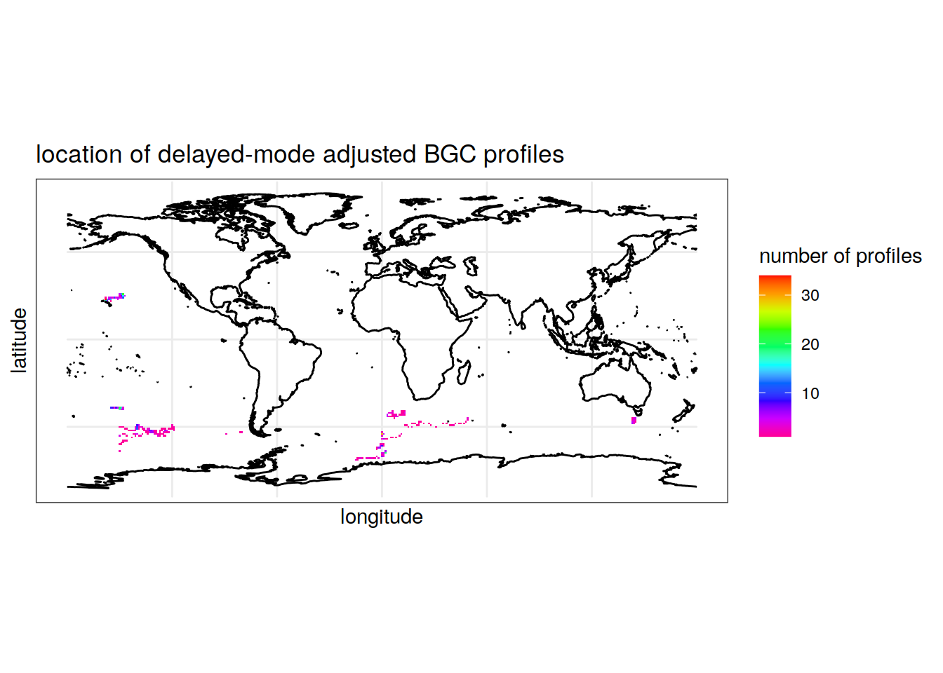

Past versions of map_bgc_profiles-1.png

Version	Author	Date
83724a0	pasqualina-vonlanthendinenna	2021-10-14

Map of profiles revised

bgc_profile_counts_year <- bgc_metadata %>% 
  select(platform_number, cycle_number, date, longitude, latitude,
         profile_doxy_qc, profile_ph_in_situ_total_qc, profile_nitrate_qc) %>% 
  pivot_longer(profile_doxy_qc:profile_nitrate_qc,
               names_to = "profile_qc",
               values_to = "flag",
               names_prefix = "profile_") %>% 
  mutate(year = year(date),
         latitude = round(latitude, digits = 0),
         longitude = round(longitude, digits = 0)) %>% 
  filter(!is.na(flag),
         flag != "") %>% 
  count(latitude, longitude, year, profile_qc)

bgc_profile_counts_flag <- bgc_metadata %>% 
  select(platform_number, cycle_number, date, longitude, latitude,
         profile_doxy_qc, profile_ph_in_situ_total_qc, profile_nitrate_qc) %>% 
  pivot_longer(profile_doxy_qc:profile_nitrate_qc,
               names_to = "profile_qc",
               values_to = "flag",
               names_prefix = "profile_") %>% 
  mutate(year = year(date),
         latitude = round(latitude, digits = 0),
         longitude = round(longitude, digits = 0)) %>% 
  filter(!is.na(flag),
         flag != "") %>% 
  count(latitude, longitude, profile_qc, flag)

Plot the evolution of the number of profiles over time

bgc_profile_counts_year %>%
  ggplot() +
  geom_sf(data = ne_countries(returnclass = "sf"),
          fill = "gray90",
          color = NA) +
  geom_sf(data = ne_coastline(returnclass = "sf")) +
  geom_tile(aes(x = longitude, y = latitude, fill = n)) +
  scale_fill_gradient(low="blue", high="red",
                      trans = "log10") +
  theme_bw() +
  facet_grid(year ~ profile_qc)

Warning: Removed 4 rows containing missing values (geom_tile).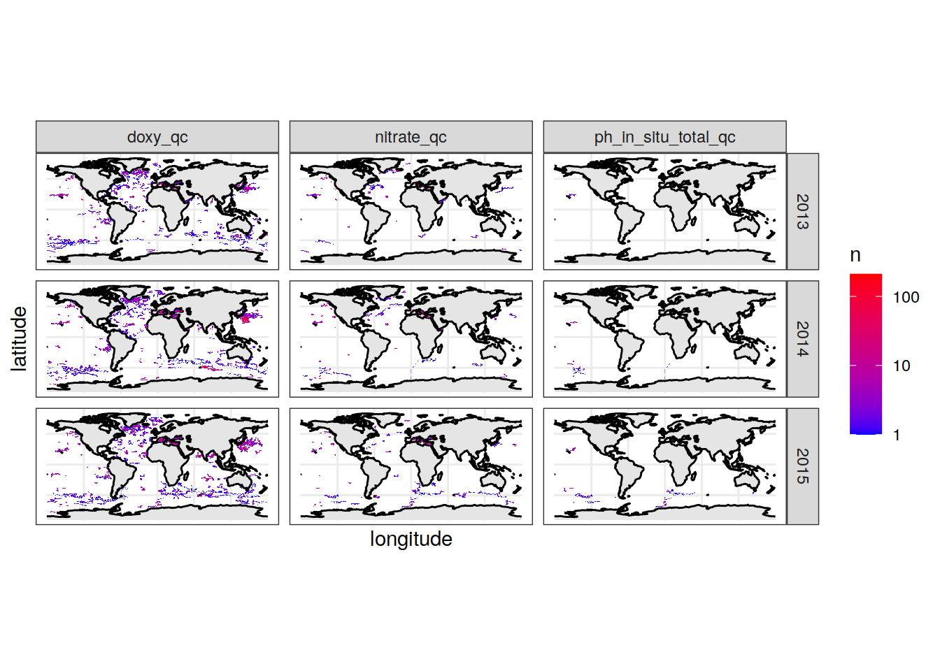

bgc_profile_counts_flag %>%
  ggplot() +
  geom_sf(data = ne_countries(returnclass = "sf"),
          fill = "gray90",
          color = NA) +
  geom_sf(data = ne_coastline(returnclass = "sf")) +
  geom_tile(aes(x = longitude, y = latitude, fill = n)) +
  scale_fill_gradient(low="blue", high="red",
                      trans = "log10") +
  theme_bw() +
  facet_grid(flag ~ profile_qc)

Warning: Removed 5 rows containing missing values (geom_tile).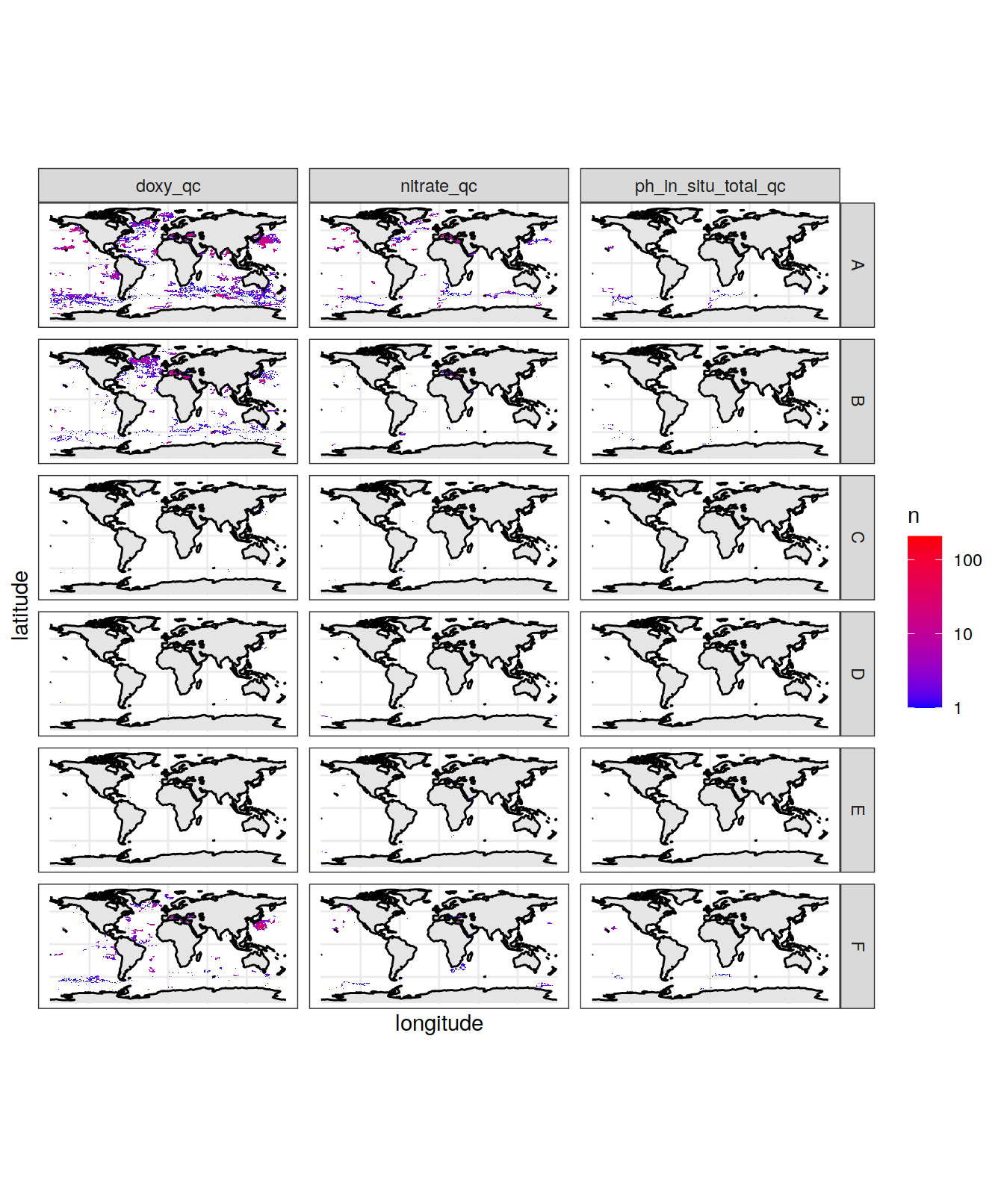

Session information

sessionInfo()

R version 4.0.3 (2020-10-10)
Platform: x86_64-pc-linux-gnu (64-bit)
Running under: openSUSE Leap 15.2

Matrix products: default
BLAS:   /usr/local/R-4.0.3/lib64/R/lib/libRblas.so
LAPACK: /usr/local/R-4.0.3/lib64/R/lib/libRlapack.so

locale:
 [1] LC_CTYPE=en_US.UTF-8       LC_NUMERIC=C              
 [3] LC_TIME=en_US.UTF-8        LC_COLLATE=en_US.UTF-8    
 [5] LC_MONETARY=en_US.UTF-8    LC_MESSAGES=en_US.UTF-8   
 [7] LC_PAPER=en_US.UTF-8       LC_NAME=C                 
 [9] LC_ADDRESS=C               LC_TELEPHONE=C            
[11] LC_MEASUREMENT=en_US.UTF-8 LC_IDENTIFICATION=C       

attached base packages:
[1] stats     graphics  grDevices utils     datasets  methods   base     

other attached packages:
 [1] rnaturalearthdata_0.1.0 rnaturalearth_0.1.0     sf_0.9-8               
 [4] lubridate_1.7.9         argodata_0.0.0.9000     forcats_0.5.0          
 [7] stringr_1.4.0           dplyr_1.0.5             purrr_0.3.4            
[10] readr_1.4.0             tidyr_1.1.3             tibble_3.1.3           
[13] ggplot2_3.3.5           tidyverse_1.3.0         workflowr_1.6.2        

loaded via a namespace (and not attached):
 [1] httr_1.4.2         sass_0.4.0         jsonlite_1.7.1     modelr_0.1.8      
 [5] bslib_0.2.5.1      assertthat_0.2.1   sp_1.4-4           highr_0.8         
 [9] blob_1.2.1         cellranger_1.1.0   yaml_2.2.1         pillar_1.6.2      
[13] backports_1.1.10   lattice_0.20-41    glue_1.4.2         digest_0.6.27     
[17] promises_1.1.1     rvest_0.3.6        colorspace_2.0-2   htmltools_0.5.1.1 
[21] httpuv_1.5.4       pkgconfig_2.0.3    broom_0.7.9        haven_2.3.1       
[25] scales_1.1.1       whisker_0.4        later_1.2.0        git2r_0.27.1      
[29] generics_0.1.0     farver_2.0.3       ellipsis_0.3.2     withr_2.3.0       
[33] cli_3.0.1          magrittr_1.5       crayon_1.3.4       readxl_1.3.1      
[37] evaluate_0.14      fs_1.5.0           fansi_0.4.1        xml2_1.3.2        
[41] class_7.3-17       tools_4.0.3        hms_0.5.3          lifecycle_1.0.0   
[45] munsell_0.5.0      reprex_0.3.0       compiler_4.0.3     jquerylib_0.1.4   
[49] e1071_1.7-4        RNetCDF_2.4-2      rlang_0.4.11       classInt_0.4-3    
[53] units_0.6-7        grid_4.0.3         rstudioapi_0.13    labeling_0.4.2    
[57] rmarkdown_2.10     gtable_0.3.0       DBI_1.1.0          R6_2.5.0          
[61] knitr_1.33         rgeos_0.5-5        utf8_1.1.4         rprojroot_2.0.2   
[65] KernSmooth_2.23-17 stringi_1.5.3      Rcpp_1.0.5         vctrs_0.3.8       
[69] dbplyr_1.4.4       tidyselect_1.1.0   xfun_0.25