Materials for publication
Jens Daniel Müller
27 May, 2021
Last updated: 2021-05-27
Checks: 7 0
Knit directory: emlr_obs_analysis/
This reproducible R Markdown analysis was created with workflowr (version 1.6.2). The Checks tab describes the reproducibility checks that were applied when the results were created. The Past versions tab lists the development history.
Great! Since the R Markdown file has been committed to the Git repository, you know the exact version of the code that produced these results.
Great job! The global environment was empty. Objects defined in the global environment can affect the analysis in your R Markdown file in unknown ways. For reproduciblity it’s best to always run the code in an empty environment.
The command set.seed(20210412) was run prior to running the code in the R Markdown file. Setting a seed ensures that any results that rely on randomness, e.g. subsampling or permutations, are reproducible.
Great job! Recording the operating system, R version, and package versions is critical for reproducibility.
Nice! There were no cached chunks for this analysis, so you can be confident that you successfully produced the results during this run.
Great job! Using relative paths to the files within your workflowr project makes it easier to run your code on other machines.
Great! You are using Git for version control. Tracking code development and connecting the code version to the results is critical for reproducibility.
The results in this page were generated with repository version f403434. See the Past versions tab to see a history of the changes made to the R Markdown and HTML files.
Note that you need to be careful to ensure that all relevant files for the analysis have been committed to Git prior to generating the results (you can use wflow_publish or wflow_git_commit). workflowr only checks the R Markdown file, but you know if there are other scripts or data files that it depends on. Below is the status of the Git repository when the results were generated:
Ignored files:
    Ignored:    .Rhistory
    Ignored:    .Rproj.user/
    Ignored:    data/
    Ignored:    output/Gruber_2019_comparison/
    Ignored:    output/publication/

Untracked files:
    Untracked:  code/Workflowr_project_managment.R

Unstaged changes:
    Modified:   analysis/_site.yml
Note that any generated files, e.g. HTML, png, CSS, etc., are not included in this status report because it is ok for generated content to have uncommitted changes.
These are the previous versions of the repository in which changes were made to the R Markdown (analysis/publication.Rmd) and HTML (docs/publication.html) files. If you’ve configured a remote Git repository (see ?wflow_git_remote), click on the hyperlinks in the table below to view the files as they were in that past version.
| File | Version | Author | Date | Message |
|---|---|---|---|---|
| html | 17e7230 | jens-daniel-mueller | 2021-04-23 | Build site. |
| Rmd | 63e2c99 | jens-daniel-mueller | 2021-04-23 | implement UP feedback |
| html | 7488bdd | jens-daniel-mueller | 2021-04-23 | Build site. |
| Rmd | b6e9179 | jens-daniel-mueller | 2021-04-23 | implement UP feedback |
| html | 6cebef7 | jens-daniel-mueller | 2021-04-22 | Build site. |
| Rmd | 8e3e166 | jens-daniel-mueller | 2021-04-22 | model truth bias added |
| html | 7e4e34b | jens-daniel-mueller | 2021-04-22 | Build site. |
| Rmd | c86fcdd | jens-daniel-mueller | 2021-04-22 | model truth bias added |
| html | 0a9f7a7 | jens-daniel-mueller | 2021-04-22 | Build site. |
| Rmd | 9a89eb9 | jens-daniel-mueller | 2021-04-22 | model truth bias added |
| html | 151be53 | jens-daniel-mueller | 2021-04-22 | Build site. |
| Rmd | 656d1e2 | jens-daniel-mueller | 2021-04-22 | model truth bias added |
| html | 8a0c4d6 | jens-daniel-mueller | 2021-04-22 | Build site. |
| Rmd | 1d621cb | jens-daniel-mueller | 2021-04-22 | model truth bias added |
| html | 5758680 | jens-daniel-mueller | 2021-04-22 | Build site. |
| Rmd | 26c1939 | jens-daniel-mueller | 2021-04-22 | model truth bias added |
| html | 3bb60c7 | jens-daniel-mueller | 2021-04-22 | Build site. |
| Rmd | 9da882f | jens-daniel-mueller | 2021-04-22 | zonal mean section added |
| html | 2cc294a | jens-daniel-mueller | 2021-04-21 | Build site. |
| Rmd | 728b5c5 | jens-daniel-mueller | 2021-04-21 | revised histogram |
| html | e336d01 | jens-daniel-mueller | 2021-04-19 | Build site. |
| Rmd | 5f76a71 | jens-daniel-mueller | 2021-04-19 | zonal mean sections added |
| html | 0e9a91d | jens-daniel-mueller | 2021-04-16 | Build site. |
| Rmd | d4af2c2 | jens-daniel-mueller | 2021-04-16 | refined inventory map |
| html | 2ab1b25 | jens-daniel-mueller | 2021-04-15 | Build site. |
| Rmd | 974c6c1 | jens-daniel-mueller | 2021-04-15 | refined inventory map |
| html | 7be394f | jens-daniel-mueller | 2021-04-15 | Build site. |
| Rmd | 71e6c6f | jens-daniel-mueller | 2021-04-15 | add publication figures |
| html | 117a5c3 | jens-daniel-mueller | 2021-04-14 | Build site. |
| Rmd | 56f179d | jens-daniel-mueller | 2021-04-14 | add publication figures |
1 Data sources
Following Cant estimates are used:
- Zonal mean (basin, lat, depth)
- Inventories (lat, lon)
cant_inv <-
  read_csv(paste(path_version_data,
                 "cant_inv.csv",
                 sep = ""))

cant_inv_mod_truth <-
  read_csv(paste(path_version_data,
                 "cant_inv_mod_truth.csv",
                 sep = ""))

cant_inv <- bind_rows(cant_inv, cant_inv_mod_truth)


cant_zonal <-
  read_csv(paste(path_version_data,
                 "cant_zonal.csv",
                 sep = ""))

cant_zonal_mod_truth <-
  read_csv(paste(path_version_data,
                 "cant_zonal_mod_truth.csv",
                 sep = ""))

cant_zonal <- bind_rows(cant_zonal,
                        cant_zonal_mod_truth)


GLODAP_clean <-
  read_csv(paste(path_version_data,
                 "GLODAPv2.2020_clean.csv",
                 sep = ""))

GLODAP_preprocessed <-
  read_csv(
    paste(
      path_preprocessing_model,
      "GLODAPv2.2020_preprocessed_model_runA_both.csv",
      sep = ""
    )
  )

GLODAP_grid_dup <-
  read_csv(paste(path_version_data,
                  "GLODAPv2.2020_clean_obs_grid_duplicates.csv",
                  sep = ""))


tref <-
  read_csv(paste(path_version_data,
                 "tref.csv",
                 sep = ""))
cant_inv <- cant_inv %>%
filter(inv_depth == params_global$inventory_depth_standard)2 Observations
2.1 Inventory map
# coastlines and worldmap

coastlines <- ne_coastline(scale = "small", returnclass = "sf")
coastlines_re <- ne_coastline(scale = "small", returnclass = "sf")
worldmap <- ne_countries(scale = "small", returnclass = "sf")
worldmap_re <- ne_countries(scale = "small", returnclass = "sf")

crs <- st_crs(coastlines)

st_geometry(worldmap_re) <- st_geometry(worldmap_re) + c(360, 0)
st_crs(worldmap_re) <- crs
worldmap <- rbind(worldmap, worldmap_re)
rm(worldmap_re)

st_geometry(coastlines_re) <- st_geometry(coastlines_re) + c(360, 0)
st_crs(coastlines_re) <- crs
coastlines <- rbind(coastlines, coastlines_re)
rm(coastlines_re)

# coastlines_buffer <- st_buffer(coastlines, dist = 1)
# coastlines_re_buffer <- st_buffer(coastlines_re, dist = 1)

# coastline_raster <- stars::st_rasterize(coastlines, options = "ALL_TOUCHED=TRUE") %>%
#   as.tibble()


# unmapped regions shape files

for (i_file in list.files("data/iho_marginal_seas")) {
  iho <- st_read(paste0("data/iho_marginal_seas/", i_file, "/iho.shp"))

  if (exists("marine_polys")) {
    marine_polys <- rbind(marine_polys, iho)
  } else {
    marine_polys <- iho
  }

}
Reading layer `iho' from data source `/UP_home/jenmueller/Projects/emlr_cant/observations/emlr_obs_analysis/data/iho_marginal_seas/baltic_sea/iho.shp' using driver `ESRI Shapefile'
Simple feature collection with 5 features and 10 fields
Geometry type: POLYGON
Dimension: XY
Bounding box: xmin: 9.365596 ymin: 52.65352 xmax: 37.46891 ymax: 67.08059
Geodetic CRS: WGS 84
Reading layer `iho' from data source `/UP_home/jenmueller/Projects/emlr_cant/observations/emlr_obs_analysis/data/iho_marginal_seas/caribbean_sea/iho.shp' using driver `ESRI Shapefile'
Simple feature collection with 1 feature and 10 fields
Geometry type: POLYGON
Dimension: XY
Bounding box: xmin: -89.41293 ymin: 7.709799 xmax: -59.4216 ymax: 22.70652
Geodetic CRS: WGS 84
Reading layer `iho' from data source `/UP_home/jenmueller/Projects/emlr_cant/observations/emlr_obs_analysis/data/iho_marginal_seas/gulf_of_mexico/iho.shp' using driver `ESRI Shapefile'
Simple feature collection with 1 feature and 10 fields
Geometry type: POLYGON
Dimension: XY
Bounding box: xmin: -98.05392 ymin: 17.40681 xmax: -80.43304 ymax: 31.46484
Geodetic CRS: WGS 84
Reading layer `iho' from data source `/UP_home/jenmueller/Projects/emlr_cant/observations/emlr_obs_analysis/data/iho_marginal_seas/hudson_bay/iho.shp' using driver `ESRI Shapefile'
Simple feature collection with 1 feature and 10 fields
Geometry type: POLYGON
Dimension: XY
Bounding box: xmin: -95.34617 ymin: 51.14359 xmax: -75.88438 ymax: 66.02643
Geodetic CRS: WGS 84
Reading layer `iho' from data source `/UP_home/jenmueller/Projects/emlr_cant/observations/emlr_obs_analysis/data/iho_marginal_seas/mediterranean_sea/iho.shp' using driver `ESRI Shapefile'
Simple feature collection with 10 features and 10 fields
Geometry type: POLYGON
Dimension: XY
Bounding box: xmin: -6.032549 ymin: 30.06809 xmax: 36.21573 ymax: 45.80891
Geodetic CRS: WGS 84
Reading layer `iho' from data source `/UP_home/jenmueller/Projects/emlr_cant/observations/emlr_obs_analysis/data/iho_marginal_seas/persian_gulf/iho.shp' using driver `ESRI Shapefile'
Simple feature collection with 1 feature and 10 fields
Geometry type: POLYGON
Dimension: XY
Bounding box: xmin: 47.70244 ymin: 23.95901 xmax: 57.33998 ymax: 31.18586
Geodetic CRS: WGS 84
Reading layer `iho' from data source `/UP_home/jenmueller/Projects/emlr_cant/observations/emlr_obs_analysis/data/iho_marginal_seas/red_sea/iho.shp' using driver `ESRI Shapefile'
Simple feature collection with 1 feature and 10 fields
Geometry type: POLYGON
Dimension: XY
Bounding box: xmin: 33.63937 ymin: 12.45626 xmax: 43.50552 ymax: 28.13954
Geodetic CRS: WGS 84marine_polys_re <- marine_polys
st_geometry(marine_polys_re) <- st_geometry(marine_polys) + c(360, 0)
st_crs(marine_polys) <- crs
st_crs(marine_polys_re) <- crs
marine_polys <- rbind(marine_polys, marine_polys_re)
rm(marine_polys_re)
# plot(st_geometry(marine_polys))
# ggplot() +
# geom_sf(data = st_geometry(marine_polys), fill = "white")
# marine_polys_simple <- st_simplify(marine_polys, dTolerance = 0.5)
# ggplot() +
# geom_sf(data = marine_polys, fill = "red") +
# geom_sf(data = marine_polys_simple, fill = "white")
black_sea <- st_read("data/black_sea/provinces.shp")Reading layer `provinces' from data source `/UP_home/jenmueller/Projects/emlr_cant/observations/emlr_obs_analysis/data/black_sea/provinces.shp' using driver `ESRI Shapefile'
Simple feature collection with 1 feature and 7 fields
Geometry type: POLYGON
Dimension: XY
Bounding box: xmin: 27.44959 ymin: 40.91028 xmax: 41.77609 ymax: 47.28054
Geodetic CRS: WGS 84black_sea_re <- black_sea
st_geometry(black_sea_re) <- st_geometry(black_sea) + c(360, 0)
st_crs(black_sea) <- crs
st_crs(black_sea_re) <- crs
black_sea <- rbind(black_sea, black_sea_re)
rm(black_sea_re)
hudson_bay <- st_read("data/hudson_bay/lme.shp")Reading layer `lme' from data source `/UP_home/jenmueller/Projects/emlr_cant/observations/emlr_obs_analysis/data/hudson_bay/lme.shp' using driver `ESRI Shapefile'
Simple feature collection with 1 feature and 16 fields
Geometry type: MULTIPOLYGON
Dimension: XY
Bounding box: xmin: -94.99611 ymin: 50.72388 xmax: -64.5891 ymax: 70.68027
Geodetic CRS: WGS 84hudson_bay_re <- hudson_bay
st_geometry(hudson_bay_re) <- st_geometry(hudson_bay) + c(360, 0)
st_crs(hudson_bay) <- crs
st_crs(hudson_bay_re) <- crs
hudson_bay <- rbind(hudson_bay, hudson_bay_re)
rm(hudson_bay_re)
caspian_sea <- st_read("data/caspian_sea/seavox_v17.shp")Reading layer `seavox_v17' from data source `/UP_home/jenmueller/Projects/emlr_cant/observations/emlr_obs_analysis/data/caspian_sea/seavox_v17.shp' using driver `ESRI Shapefile'
Simple feature collection with 1 feature and 20 fields
Geometry type: POLYGON
Dimension: XY
Bounding box: xmin: 46.6797 ymin: 36.5801 xmax: 54.7659 ymax: 47.1153
Geodetic CRS: WGS 84caspian_sea_re <- caspian_sea
st_geometry(caspian_sea_re) <- st_geometry(caspian_sea) + c(360, 0)
st_crs(caspian_sea) <- crs
st_crs(caspian_sea_re) <- crs
caspian_sea <- rbind(caspian_sea, caspian_sea_re)
rm(caspian_sea_re)
# ggplot() +
# geom_sf(data = marine_polys, fill = "white") +
# geom_sf(data = black_sea, fill = "white") +
# geom_sf(data = caspian_sea, fill = "white") +
# geom_sf(data = hudson_bay, fill = "white")set_breaks <- c(-Inf, seq(0, 10, 2), Inf)
color_land <- "grey80"
color_unmapped <- "grey90"
var_name <- expression(atop(Delta * C["ant"],
(mol ~ m ^ {
-2
})))
GLODAP_grid_both <- GLODAP_grid_dup %>%
filter(duplicate == "no") %>%
distinct(lon, lat, era)
p_inv_map <- ggplot() +
geom_contour_fill(
data = cant_inv %>% filter(data_source == "obs"),
aes(lon, lat, z = cant_inv, fill = stat(level)),
breaks = set_breaks,
na.fill = TRUE
) +
scale_fill_viridis_d(option = "D", name = var_name,
guide = guide_colorsteps(barheight = 10)) +
new_scale_fill() +
geom_tile(data = GLODAP_grid_both,
aes(x = lon, y = lat, height = 0.7, width = 0.7, fill=era)) +
scale_fill_manual(values = c("Deeppink4", "Deeppink"),
name = "Decade", guide = FALSE) +
geom_sf(data = marine_polys, fill = color_unmapped, col="transparent") +
geom_sf(data = black_sea, fill = color_unmapped, col="transparent") +
geom_sf(data = caspian_sea, fill = color_unmapped, col="transparent") +
geom_sf(data = hudson_bay, fill = "white", col="white") +
geom_sf(data = worldmap, fill = color_land, col="transparent") +
geom_sf(data = coastlines, col = "black") +
coord_sf(ylim = c(-77.5,64.5), xlim = c(20.5,379.5), expand = 0) +
labs(title = expression("Column inventory (0 - 3000m) of the change in anthropogenic CO"[2]~
"from 2006 to 2014")) +
theme(axis.text = element_blank(),
axis.ticks = element_blank(),
axis.title = element_blank(),
legend.key = element_rect(colour = "black"))
ggsave(plot = p_inv_map,
path = "output/publication",
filename = "dCant_inventory_map.png",
height = 4,
width = 10)2.2 Time series histogram
time_histo <- GLODAP_preprocessed %>%
  filter(!is.na(tco2)) %>%
  count(year)

p_time_histo <-
  ggplot() +
  geom_col(data = time_histo %>% filter(year < 2000),
           aes(year, n, fill = "era1"),
           col = "grey20") +
  geom_col(
    data = time_histo %>% filter(year >= 2000, year < 2010),
    aes(year, n, fill = "era2"),
    col = "grey20"
  ) +
  geom_col(data = time_histo %>% filter(year >= 2010),
           aes(year, n, fill = "era3"),
           col = "grey20") +
  scale_fill_manual(values = c("grey", "Deeppink4", "Deeppink"),
                    name = "Decade", guide = FALSE) +
  scale_x_continuous(breaks = seq(1900, 2100, 5)) +
  scale_y_continuous(limits = c(0, max(time_histo$n)+500)) +
  coord_cartesian(expand = 0) +
  labs(title = "GLODAPv2.2020 | Observations per year") +
  theme_classic() +
  theme(axis.title = element_blank())


p_time_histo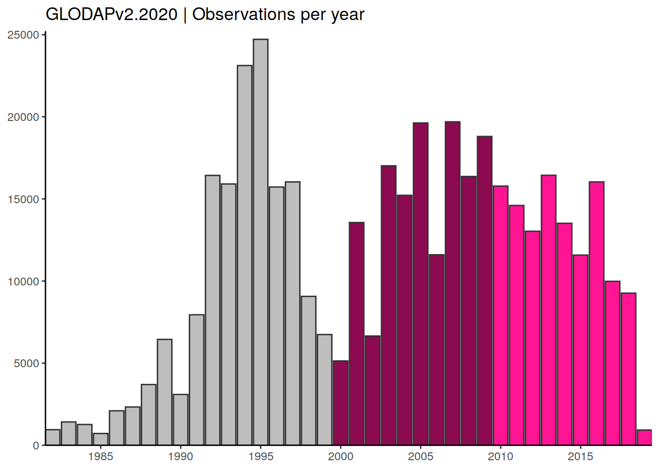
ggsave(plot = p_time_histo,
       path = "output/publication",
       filename = "time_histo.png",
       height = 2,
       width = 10)
2.3 Spatial time coverage
time_histo <- GLODAP_preprocessed %>%
  filter(year >= 2000) %>%
  distinct(lat, lon, year)

p_coverage_maps <-
map +
  geom_raster(data = time_histo, aes(lon, lat)) +
  facet_wrap( ~ year) +
  theme(
    axis.text = element_blank(),
    axis.ticks = element_blank(),
    axis.title = element_blank()
  )

p_coverage_maps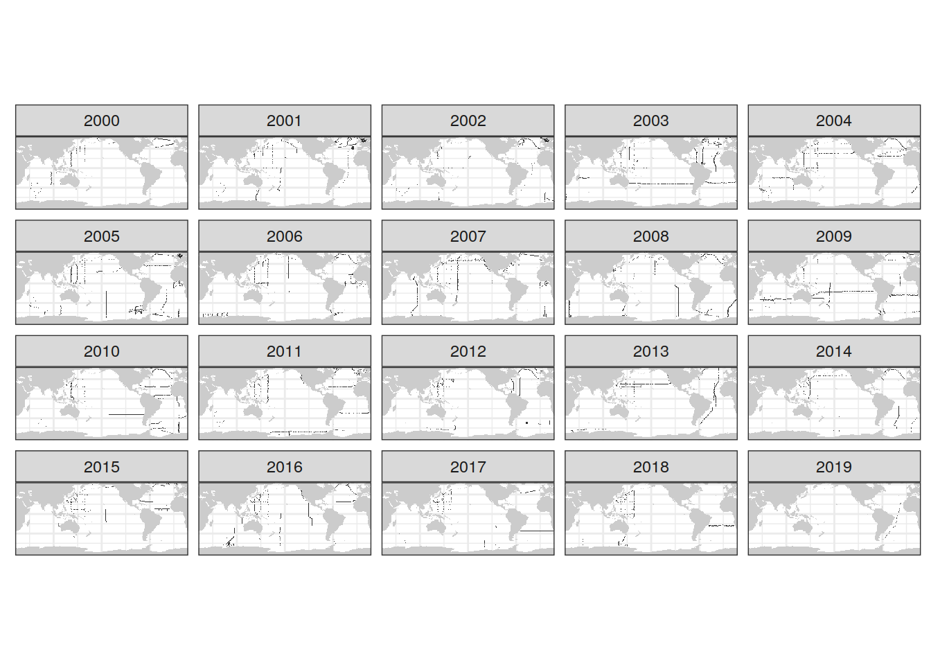
| Version | Author | Date |
|---|---|---|
| 6cebef7 | jens-daniel-mueller | 2021-04-22 |
ggsave(plot = p_coverage_maps,
       path = "output/publication",
       filename = "data_coverage_maps_by_year.png",
       height = 7,
       width = 16)
time_histo <- GLODAP_preprocessed %>%
filter(year >= 2000) %>%
distinct(lat, lon, year)
GLODAP_grid_both <- GLODAP_grid_dup %>%
filter(duplicate == "no") %>%
count(lon, lat) %>%
mutate(n = as.factor(n))
p_coverage_maps <-
ggplot() +
geom_raster(data = GLODAP_grid_both,
aes(x = lon, y = lat, fill = n)) +
scale_fill_brewer(palette = "Set1",
name = "Decades\noccupied",
direction = -1) +
geom_sf(data = worldmap, fill = color_land, col = "transparent") +
geom_sf(data = coastlines, col = "black") +
coord_sf(
ylim = c(-77.5, 64.5),
xlim = c(20.5, 379.5),
expand = 0
) +
labs(title = "GLODAPv2.2020 | Data coverage in the post-2000 era") +
theme(
axis.text = element_blank(),
axis.ticks = element_blank(),
axis.title = element_blank(),
legend.key = element_rect(colour = "black"),
panel.grid = element_blank()
)
p_coverage_maps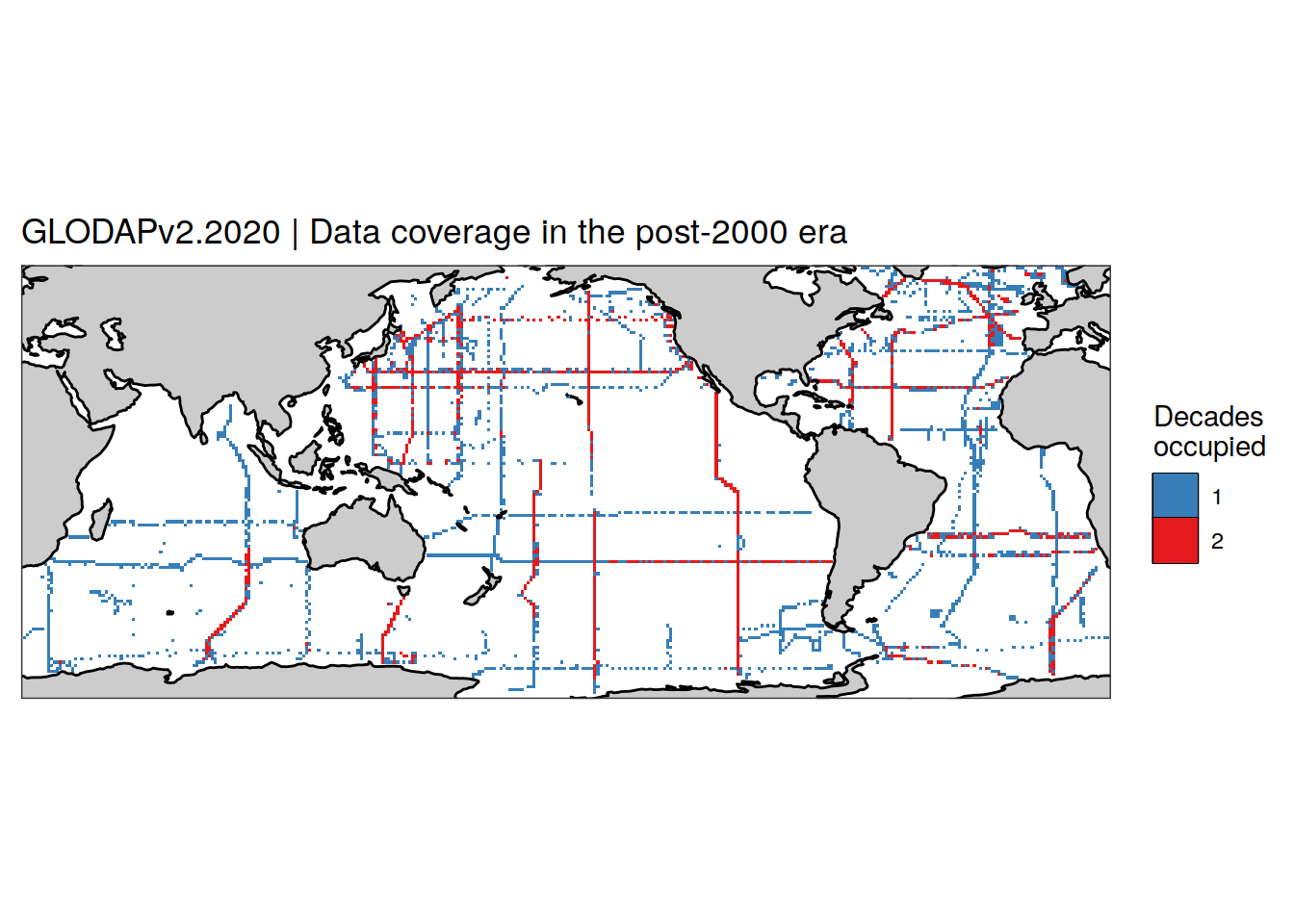
ggsave(plot = p_coverage_maps,
       path = "output/publication",
       filename = "data_coverage_map_post_2000.png",
       height = 4,
       width = 10)
p_coverage_maps <-
ggplot() +
geom_raster(data = GLODAP_grid_dup,
aes(x = lon, y = lat, fill = duplicate)) +
scale_fill_brewer(palette = "Set1",
name = "Duplicated\ndata",
direction = -1) +
geom_sf(data = worldmap, fill = color_land, col = "transparent") +
geom_sf(data = coastlines, col = "black") +
coord_sf(
ylim = c(-77.5, 64.5),
xlim = c(20.5, 379.5),
expand = 0
) +
facet_wrap(~ era, ncol = 1) +
theme(
axis.text = element_blank(),
axis.ticks = element_blank(),
axis.title = element_blank(),
legend.key = element_rect(colour = "black"),
panel.grid = element_blank()
)
p_coverage_maps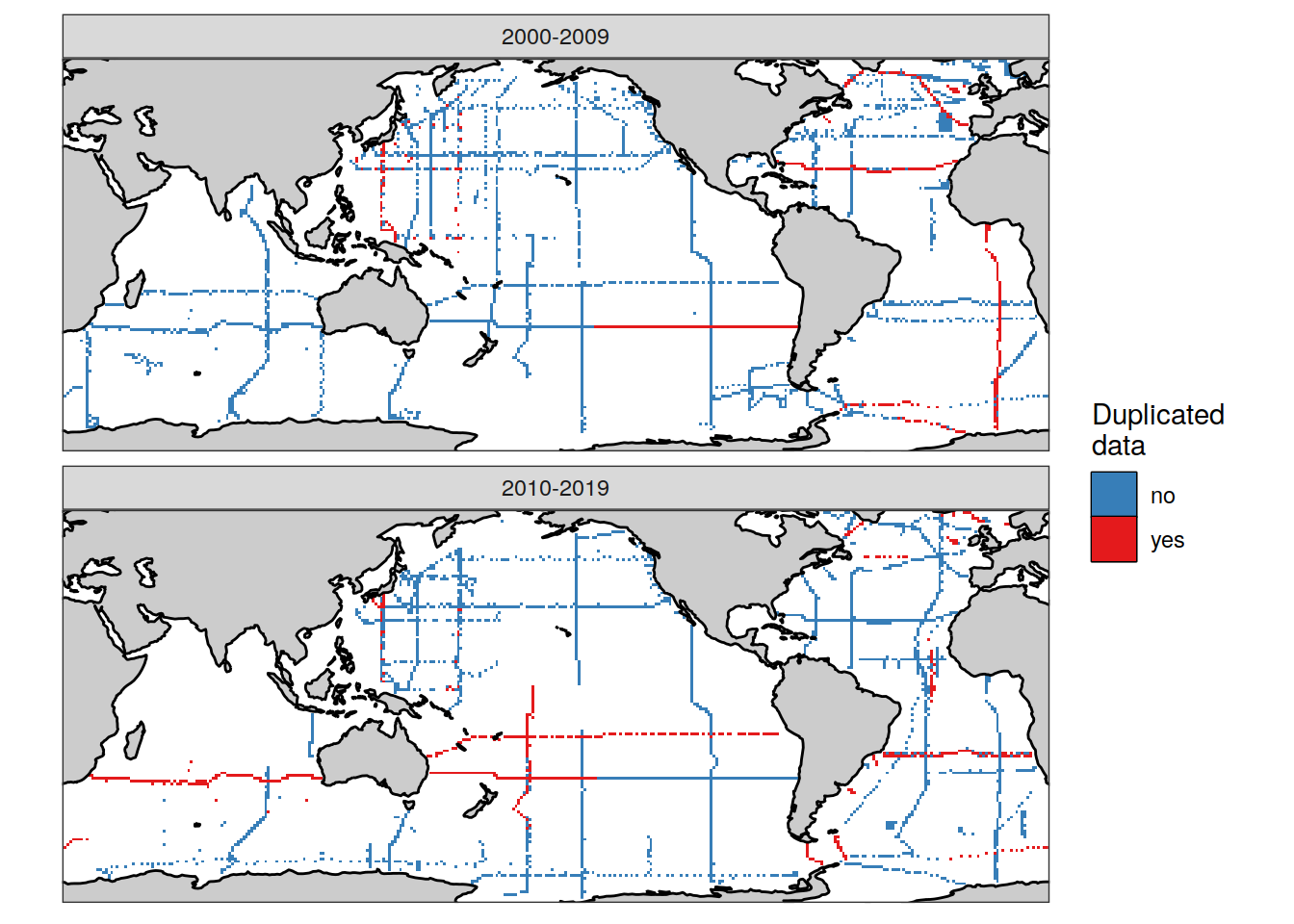
ggsave(plot = p_coverage_maps,
       path = "output/publication",
       filename = "data_coverage_map_duplicated_data.png",
       height = 6,
       width = 7)
color_land <- "white"
color_unmapped <- "white"
p_inv_map <- ggplot() +
geom_contour_fill(
data = cant_inv %>% filter(data_source == "obs"),
aes(lon, lat, z = cant_inv, fill = stat(level)),
breaks = set_breaks,
na.fill = TRUE
) +
scale_fill_viridis_d(option = "D", name = var_name,
guide = FALSE) +
geom_sf(data = marine_polys, fill = color_unmapped, col="transparent") +
geom_sf(data = black_sea, fill = color_unmapped, col="transparent") +
geom_sf(data = caspian_sea, fill = color_unmapped, col="transparent") +
geom_sf(data = hudson_bay, fill = "white", col="white") +
geom_sf(data = worldmap, fill = color_land, col="transparent") +
geom_sf(data = coastlines, col = "white") +
coord_sf(ylim = c(-77.5,64.5), xlim = c(20.5,379.5), expand = 0) +
theme_void()
ggsave(plot = p_inv_map,
path = "output/publication",
filename = "dCant_inventory_map_color_only.png",
height = 4,
width = 10)2.4 Uptake rate comparison
cant_inv_budget <- cant_inv %>%
  mutate(surface_area = earth_surf(lat, lon),
         cant_inv_grid = cant_inv*surface_area,
         cant_pos_inv_grid = cant_pos_inv*surface_area) %>%
  group_by(basin_AIP, data_source, inv_depth) %>%
  summarise(cant_total = sum(cant_inv_grid)*12*1e-15,
            cant_total = round(cant_total,1),
            cant_pos_total = sum(cant_pos_inv_grid)*12*1e-15,
            cant_pos_total = round(cant_pos_total,1)) %>%
  ungroup()

duration <- sort(tref$median_year)[2] - sort(tref$median_year)[1]

cant_inv_budget_obs <- cant_inv_budget %>%
  filter(data_source == "obs",
         inv_depth == 3000) %>%
  summarise(cant_uptake_rate = sum(cant_total)/duration) %>%
  mutate(source = "Interior\nstorage",
         period = "This study",
         uncertainty = 0.3)

cant_inv_budget_lit <-
  bind_cols(
    cant_uptake_rate = c(2.37, 2.18 + 0.61),
    source = c("Ocean\nmodels", "Observed\nfluxes"),
    period = c("Global\nCarbon Budget", "Global\nCarbon Budget"),
    uncertainty = c(0.6, 0.6)
  )

cant_inv_budget_all <- bind_rows(
  cant_inv_budget_obs,
  cant_inv_budget_lit
)


p_budget <-
  cant_inv_budget_all %>%
  ggplot() +
  geom_col(aes(source, cant_uptake_rate),
           fill = "grey80",
           col = "grey20") +
  geom_errorbar(
    aes(
      x = source,
      ymin = cant_uptake_rate - uncertainty,
      ymax = cant_uptake_rate + uncertainty
    ),
    width = .2
  ) +
    geom_text(
    aes(
      x = source,
      y = 0.8,
      label = period,
      angle = 90
    )
  ) +
  scale_y_continuous(limits = c(
    0,
    max(
      cant_inv_budget_all$cant_uptake_rate +
        cant_inv_budget_all$uncertainty
    ) + 0.1
  ),
  expand = c(0, 0)) +
  labs(title = "Ocean carbon sink 2006 - 2014",
       y = expression(Average~rate ~ (PgC ~ yr ^ {-1}))) +
  theme_classic() +
  theme(axis.title.x = element_blank(),
        panel.grid = element_blank())


p_budget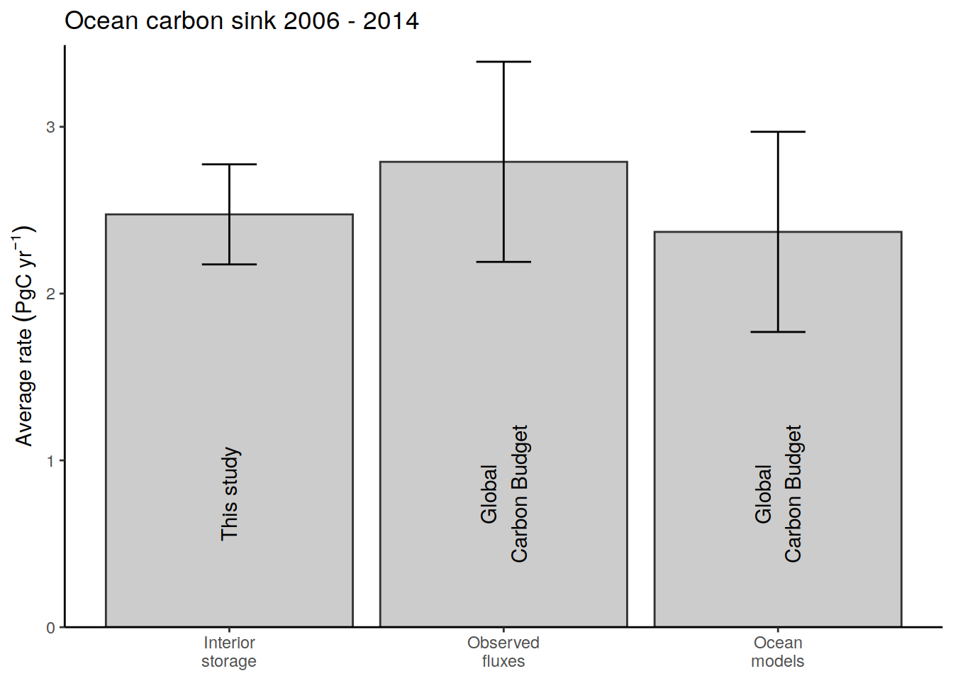
ggsave(plot = p_budget,
       path = "output/publication",
       filename = "uptake_rate_comparison.png",
       height = 3.5,
       width = 3.5)
2.5 Zonal mean sections
breaks <- c(-Inf, seq(0, 10, 1), Inf)
breaks_n <- length(breaks) - 1

legend_title = expression(atop(Delta * C[ant, pos],
                               (mu * mol ~ kg ^ {
                                 -1
                               })))

i_basin_AIP <- "Atlantic"
slab_breaks <- params_local$slabs_Atl
i_data_source <- "obs"

# plot base section
section <-
  cant_zonal %>%
  filter(basin_AIP == i_basin_AIP,
         data_source == i_data_source) %>%
  ggplot() +
  guides(fill = FALSE) +
  scale_y_reverse() +
  scale_x_continuous(breaks = seq(-100, 100, 20),
                     limits = c(min(cant_zonal$lat), max(cant_zonal$lat))) +
  geom_contour_filled(aes(lat, depth, z = cant_mean),
                      breaks = breaks) +
  scale_fill_viridis_d(name = legend_title) +
  geom_hline(yintercept = params_local$depth_min,
             col = "white",
             linetype = 2) +
  geom_contour(aes(lat, depth, z = gamma_mean),
               breaks = slab_breaks,
               col = "white") +
  geom_text_contour(
    aes(lat, depth, z = gamma_mean),
    breaks = slab_breaks,
    col = "white",
    skip = 2
  )

# cut surface water section
surface <-
  section +
  coord_cartesian(expand = 0,
                  ylim = c(500, 0)) +
  labs(y = "Depth (m)",
       title =paste(i_basin_AIP, "Ocean")) +
  theme(
    axis.title.x = element_blank(),
    axis.text.x = element_blank(),
    axis.ticks.x = element_blank()
  )

# cut deep water section
deep <-
  section +
  coord_cartesian(expand = 0,
                  ylim = c(params_global$inventory_depth_standard, 500)) +
  labs(x = expression(latitude ~ (degree * N)), y = "Depth (m)")


# combine surface and deep water section
section_combined_Atl <-
  surface / deep +
  plot_layout(guides = "collect")

section_combined_Atl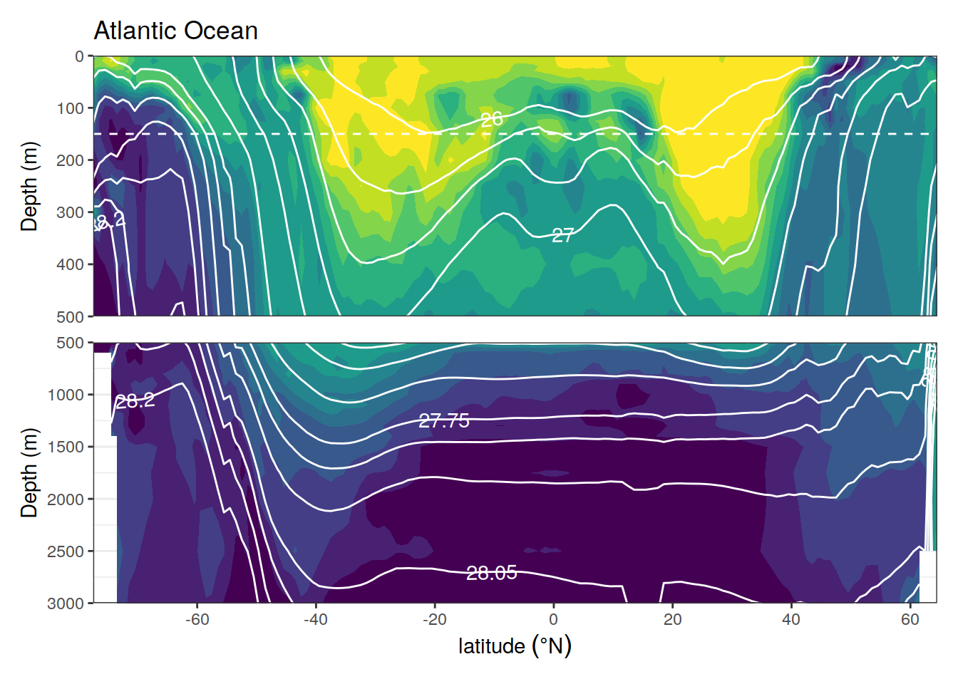
i_basin_AIP <- "Pacific"
slab_breaks <- params_local$slabs_Ind_Pac

# plot base section
section <-
  cant_zonal %>%
  filter(basin_AIP == i_basin_AIP,
         data_source == i_data_source) %>%
  ggplot() +
  guides(fill = FALSE) +
  scale_y_reverse() +
  scale_x_continuous(breaks = seq(-100, 100, 20),
                     limits = c(min(cant_zonal$lat), max(cant_zonal$lat))) +
  geom_contour_filled(aes(lat, depth, z = cant_mean),
                      breaks = breaks) +
  scale_fill_viridis_d(name = legend_title) +
  geom_hline(yintercept = params_local$depth_min,
             col = "white",
             linetype = 2) +
  geom_contour(aes(lat, depth, z = gamma_mean),
               breaks = slab_breaks,
               col = "white") +
  geom_text_contour(
    aes(lat, depth, z = gamma_mean),
    breaks = slab_breaks,
    col = "white",
    skip = 2
  )

# cut surface water section
surface <-
  section +
  coord_cartesian(expand = 0,
                  ylim = c(500, 0)) +
  labs(y = "Depth (m)",
       title =paste(i_basin_AIP, "Ocean")) +
  theme(
    axis.title = element_blank(),
    axis.text = element_blank(),
    axis.ticks = element_blank()
  )

# cut deep water section
deep <-
  section +
  coord_cartesian(expand = 0,
                  ylim = c(params_global$inventory_depth_standard, 500)) +
  labs(x = expression(latitude ~ (degree * N)), y = "Depth (m)") +
  theme(
    axis.title.y = element_blank(),
    axis.text.y = element_blank(),
    axis.ticks.y = element_blank()
  )


# combine surface and deep water section
section_combined_Pac <-
  surface / deep +
  plot_layout(guides = "collect")

section_combined_Pac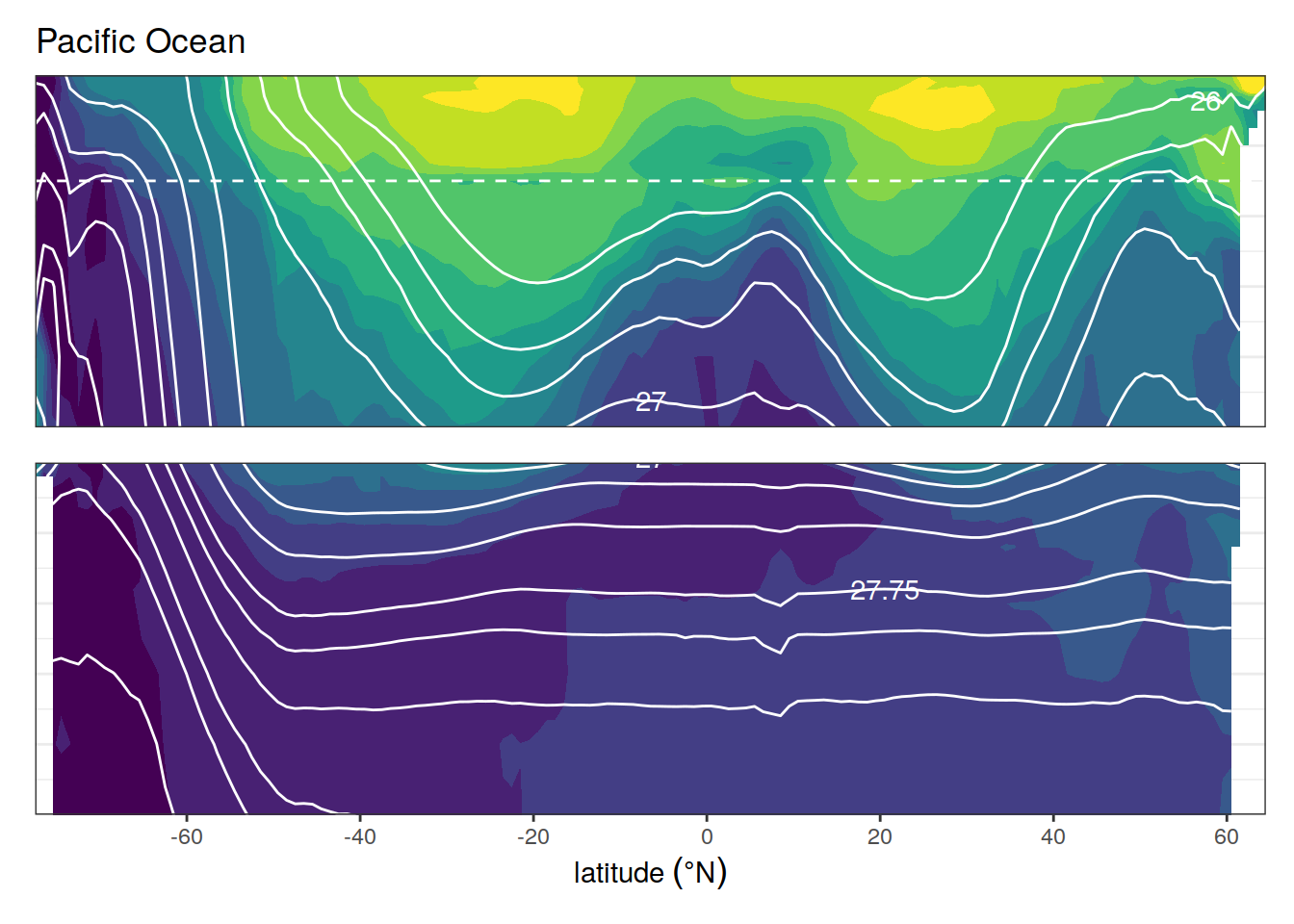
| Version | Author | Date |
|---|---|---|
| 5758680 | jens-daniel-mueller | 2021-04-22 |
i_basin_AIP <- "Indian"
slab_breaks <- params_local$slabs_Ind_Pac

# plot base section
section <-
  cant_zonal %>%
  filter(basin_AIP == i_basin_AIP,
         data_source == i_data_source) %>%
  ggplot() +
  guides(fill = guide_colorsteps(barheight = unit(6, "cm"))) +
  scale_y_reverse() +
  scale_x_continuous(breaks = seq(-100, 100, 20),
                     limits = c(min(cant_zonal$lat), max(cant_zonal$lat))) +
  geom_contour_filled(aes(lat, depth, z = cant_mean),
                      breaks = breaks) +
  scale_fill_viridis_d(name = legend_title) +
  geom_hline(yintercept = params_local$depth_min,
             col = "white",
             linetype = 2) +
  geom_contour(aes(lat, depth, z = gamma_mean),
               breaks = slab_breaks,
               col = "white") +
  geom_text_contour(
    aes(lat, depth, z = gamma_mean),
    breaks = slab_breaks,
    col = "white",
    skip = 2
  )

# cut surface water section
surface <-
  section +
  coord_cartesian(expand = 0,
                  ylim = c(500, 0)) +
  labs(y = "Depth (m)",
       title =paste(i_basin_AIP, "Ocean")) +
  theme(
    axis.title = element_blank(),
    axis.text = element_blank(),
    axis.ticks = element_blank()
  )

# cut deep water section
deep <-
  section +
  coord_cartesian(expand = 0,
                  ylim = c(params_global$inventory_depth_standard, 500)) +
  labs(x = expression(latitude ~ (degree * N)), y = "Depth (m)") +
  theme(
    axis.title.y = element_blank(),
    axis.text.y = element_blank(),
    axis.ticks.y = element_blank()
  )


# combine surface and deep water section
section_combined_Ind <-
  surface / deep +
  plot_layout(guides = "collect")

section_combined_Ind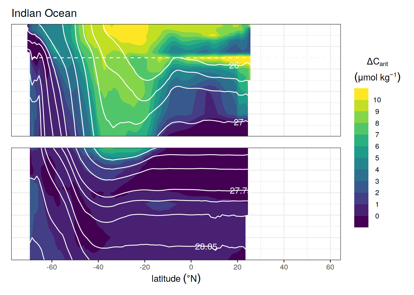
| Version | Author | Date |
|---|---|---|
| 5758680 | jens-daniel-mueller | 2021-04-22 |
section_combined <-
section_combined_Atl | section_combined_Pac | section_combined_Ind


ggsave(plot = section_combined,
       path = "output/publication",
       filename = "zonal_mean_section_obs.png",
       height = 4,
       width = 12)
3 Synthetic data
3.1 Inventory map
set_breaks <- c(-Inf, seq(0, 12, 2), Inf)
color_land <- "grey80"
color_unmapped <- "grey90"

var_name <- expression(atop(Delta * C["ant"],
                            (mol ~ m ^ {
                              -2
                            })))


p_inv_map <- ggplot() +
  geom_contour_fill(
    data = cant_inv %>% filter(data_source == "mod"),
    aes(lon, lat, z = cant_inv, fill = stat(level)),
    breaks = set_breaks,
    na.fill = TRUE
  ) +
  scale_fill_viridis_d(option = "D", name = var_name,
                       guide = guide_colorsteps()) +
  new_scale_fill() +
  geom_tile(data = GLODAP_grid_both,
              aes(x = lon, y = lat, height = 0.7, width = 0.7, fill=n)) +
  scale_fill_manual(values = c("Deeppink4", "Deeppink"),
                    name = "Eras\noccupied") +
  geom_sf(data = marine_polys, fill = color_unmapped, col="transparent") +
  geom_sf(data = black_sea,  fill = color_unmapped, col="transparent") +
  geom_sf(data = caspian_sea,  fill = color_unmapped, col="transparent") +
  geom_sf(data = hudson_bay, fill = "white", col="white") +
  geom_sf(data = worldmap,  fill = color_land, col="transparent") +
  geom_sf(data = coastlines, col = "black") +
  coord_sf(ylim = c(-77.5,64.5), xlim = c(20.5,379.5), expand = 0) +
  labs(title = expression("Column inventory (0 - 3000m) of the change in anthropogenic CO"[2]~
                            "from 2006 to 2014"),
       subtitle = "eMLR(C*) reconstruction") +
  theme(axis.text = element_blank(),
        axis.ticks = element_blank(),
        axis.title = element_blank(),
        legend.key = element_rect(colour = "black"))

# bias map

set_breaks <- c(-Inf, seq(-4, 4, 1), Inf)
var_name <- expression(atop(Delta * C["ant"]~bias,
                            (mol ~ m ^ {
                              -2
                            })))


cant_inv_bias <- cant_inv %>%
  filter(data_source %in% c("mod", "mod_truth")) %>%
  select(lat, lon, data_source, cant_inv) %>%
  pivot_wider(names_from = data_source,
              values_from = cant_inv) %>%
  mutate(cant_inv_bias = mod - mod_truth) %>%
  drop_na()


p_inv_map_bias <- ggplot() +
  geom_contour_fill(
    data = cant_inv_bias,
    aes(lon, lat, z = cant_inv_bias, fill = stat(level)),
    breaks = set_breaks,
    na.fill = TRUE
  ) +
  scale_fill_brewer(
    palette = "RdBu",
    direction = -1,
    drop = FALSE,
    name = var_name,
    guide = guide_colorsteps(barheight = unit(5, "cm"))
  ) +
  geom_sf(data = marine_polys, fill = color_unmapped, col = "transparent") +
  geom_sf(data = black_sea,  fill = color_unmapped, col = "transparent") +
  geom_sf(data = caspian_sea,  fill = color_unmapped, col = "transparent") +
  geom_sf(data = hudson_bay, fill = "white", col = "white") +
  geom_sf(data = worldmap,  fill = color_land, col = "transparent") +
  geom_sf(data = coastlines, col = "black") +
  coord_sf(
    ylim = c(-77.5, 64.5),
    xlim = c(20.5, 379.5),
    expand = 0
  ) +
  labs(subtitle = "eMLR(C*) reconstruction - model truth")+
  theme(
    axis.text = element_blank(),
    axis.ticks = element_blank(),
    axis.title = element_blank(),
    legend.key = element_rect(colour = "black")
  )

p_inv_map_mod <-
p_inv_map / p_inv_map_bias

ggsave(plot = p_inv_map_mod,
       path = "output/publication",
       filename = "dCant_inventory_map_mod_bias.png",
       height = 7,
       width = 9)
3.2 Budgets
cant_inv_budget_mod <- cant_inv_budget %>%
  filter(
    inv_depth == params_global$inventory_depth_standard,
    data_source %in% c("mod", "mod_truth")
  ) %>%
  select(-c(cant_pos_total, inv_depth))


cant_inv_budget_mod %>%
  pivot_wider(names_from = data_source,
              values_from = cant_total) %>%
  mutate(abs_bias = mod - mod_truth,
         rel_bias = ((mod / mod_truth) - 1) * 100)
# A tibble: 3 x 5
basin_AIP mod mod_truth abs_bias rel_bias
<chr> <dbl> <dbl> <dbl> <dbl>
1 Atlantic 4.6 4.1 0.5 12.2
2 Indian 2.6 4.5 -1.9 -42.2
3 Pacific 7.1 8 -0.9 -11.3cant_inv_budget_mod %>%
group_by(data_source) %>%
summarise(cant_total = sum(cant_total)) %>%
ungroup() %>%
pivot_wider(names_from = data_source,
values_from = cant_total) %>%
mutate(abs_bias = mod - mod_truth,
rel_bias = ((mod / mod_truth) - 1) * 100)# A tibble: 1 x 4
mod mod_truth abs_bias rel_bias
<dbl> <dbl> <dbl> <dbl>
1 14.3 16.6 -2.3 -13.9p_budget_comparison <-
cant_inv_budget_mod %>%
mutate(
data_source = recode(data_source,
mod = "eMLR(C*)\nreconstruction",
mod_truth = "Model\ntruth")
) %>%
ggplot(aes(data_source, cant_total, fill = basin_AIP)) +
scale_fill_brewer(palette = "Greys", name = "Ocean basin",
direction = -1) +
scale_y_continuous(limits = c(0, 18), expand = c(0, 0)) +
labs(y = expression(Delta * C["ant"] ~ (PgC)),
title = "Regionally integrated budgets") +
geom_col(col = "grey20") +
theme_bw() +
theme(axis.title.x = element_blank())
p_budget_comparison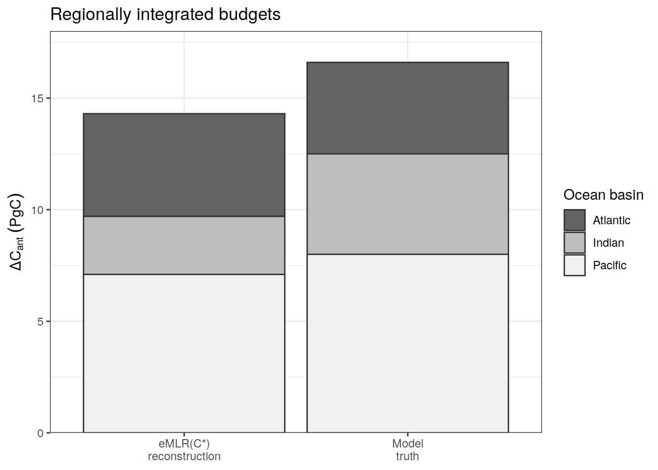
| Version | Author | Date |
|---|---|---|
| 8a0c4d6 | jens-daniel-mueller | 2021-04-22 |
ggsave(plot = p_budget_comparison,
       path = "output/publication",
       filename = "budget_comparison.png",
       height = 3.5,
       width = 4)
3.3 Zonal mean sections
3.3.1 eMLR
breaks <- c(-Inf, seq(0, 10, 1), Inf)
breaks_n <- length(breaks) - 1

legend_title = expression(atop(Delta * C[ant, pos],
                               (mu * mol ~ kg ^ {
                                 -1
                               })))

i_basin_AIP <- "Atlantic"
slab_breaks <- params_local$slabs_Atl
i_data_source <- "mod"

# plot base section
section <-
  cant_zonal %>%
  filter(basin_AIP == i_basin_AIP,
         data_source == i_data_source) %>%
  ggplot() +
  guides(fill = FALSE) +
  scale_y_reverse() +
  scale_x_continuous(breaks = seq(-100, 100, 20),
                     limits = c(min(cant_zonal$lat), max(cant_zonal$lat))) +
  geom_contour_filled(aes(lat, depth, z = cant_mean),
                      breaks = breaks) +
  scale_fill_viridis_d(name = legend_title) +
  geom_hline(yintercept = params_local$depth_min,
             col = "white",
             linetype = 2) +
  geom_contour(aes(lat, depth, z = gamma_mean),
               breaks = slab_breaks,
               col = "white") +
  geom_text_contour(
    aes(lat, depth, z = gamma_mean),
    breaks = slab_breaks,
    col = "white",
    skip = 2
  ) +
  theme(
    axis.title.x = element_blank(),
    axis.text.x = element_blank(),
    axis.ticks.x = element_blank()
  )

# cut surface water section
surface <-
  section +
  coord_cartesian(expand = 0,
                  ylim = c(500, 0)) +
  labs(y = "Depth (m)",
       title =paste(i_basin_AIP, "Ocean"))

# cut deep water section
deep <-
  section +
  coord_cartesian(expand = 0,
                  ylim = c(params_global$inventory_depth_standard, 500)) +
  labs(x = expression(latitude ~ (degree * N)), y = "Depth (m)")


# combine surface and deep water section
section_combined_Atl <-
  surface / deep +
  plot_layout(guides = "collect")

section_combined_Atl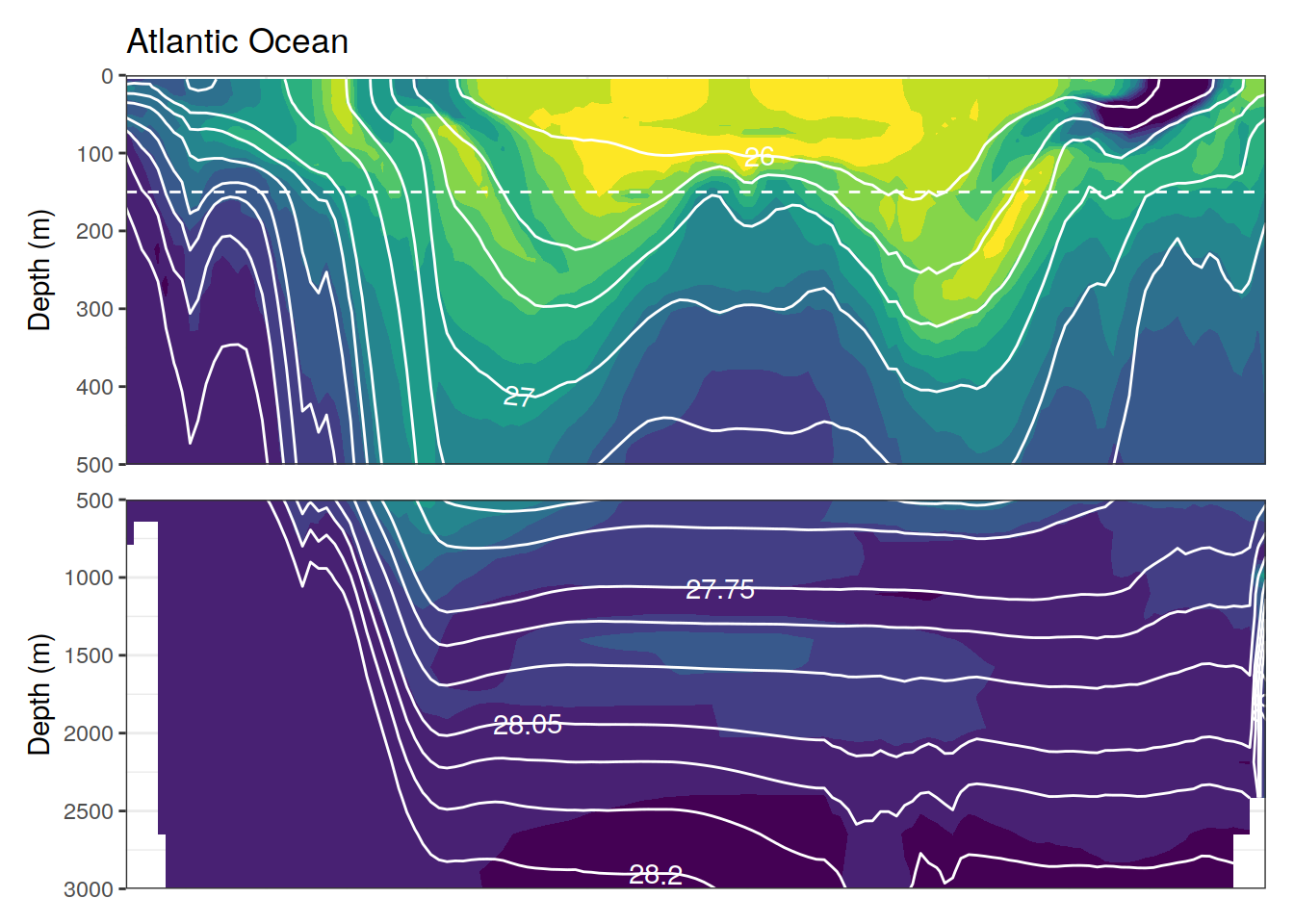
i_basin_AIP <- "Pacific"
slab_breaks <- params_local$slabs_Ind_Pac

# plot base section
section <-
  cant_zonal %>%
  filter(basin_AIP == i_basin_AIP,
         data_source == i_data_source) %>%
  ggplot() +
  guides(fill = FALSE) +
  scale_y_reverse() +
  scale_x_continuous(breaks = seq(-100, 100, 20),
                     limits = c(min(cant_zonal$lat), max(cant_zonal$lat))) +
  geom_contour_filled(aes(lat, depth, z = cant_mean),
                      breaks = breaks) +
  scale_fill_viridis_d(name = legend_title) +
  geom_hline(yintercept = params_local$depth_min,
             col = "white",
             linetype = 2) +
  geom_contour(aes(lat, depth, z = gamma_mean),
               breaks = slab_breaks,
               col = "white") +
  geom_text_contour(
    aes(lat, depth, z = gamma_mean),
    breaks = slab_breaks,
    col = "white",
    skip = 2
  ) +
  theme(
    axis.title = element_blank(),
    axis.text = element_blank(),
    axis.ticks = element_blank()
  )


# cut surface water section
surface <-
  section +
  coord_cartesian(expand = 0,
                  ylim = c(500, 0)) +
  labs(y = "Depth (m)",
       title =paste(i_basin_AIP, "Ocean"))
# cut deep water section
deep <-
  section +
  coord_cartesian(expand = 0,
                  ylim = c(params_global$inventory_depth_standard, 500)) +
  labs(x = expression(latitude ~ (degree * N)), y = "Depth (m)") +
  theme(
    axis.title.y = element_blank(),
    axis.text.y = element_blank(),
    axis.ticks.y = element_blank()
  )


# combine surface and deep water section
section_combined_Pac <-
  surface / deep +
  plot_layout(guides = "collect")

section_combined_Pac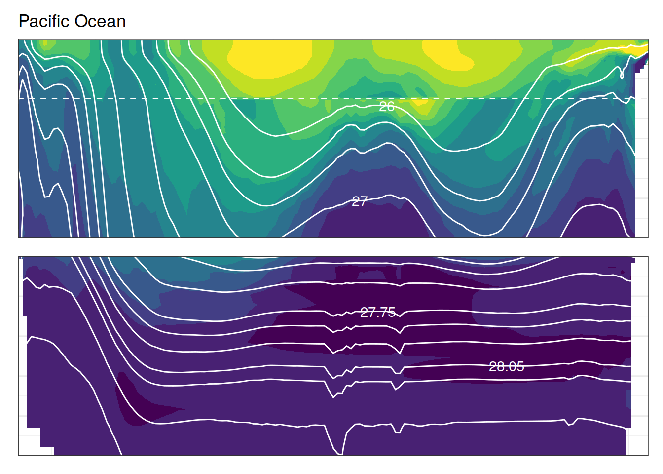
i_basin_AIP <- "Indian"
slab_breaks <- params_local$slabs_Ind_Pac

# plot base section
section <-
  cant_zonal %>%
  filter(basin_AIP == i_basin_AIP,
         data_source == i_data_source) %>%
  ggplot() +
  guides(fill = guide_colorsteps(barheight = unit(5, "cm"))) +
  scale_y_reverse() +
  scale_x_continuous(breaks = seq(-100, 100, 20),
                     limits = c(min(cant_zonal$lat), max(cant_zonal$lat))) +
  geom_contour_filled(aes(lat, depth, z = cant_mean),
                      breaks = breaks) +
  scale_fill_viridis_d(name = legend_title) +
  geom_hline(yintercept = params_local$depth_min,
             col = "white",
             linetype = 2) +
  geom_contour(aes(lat, depth, z = gamma_mean),
               breaks = slab_breaks,
               col = "white") +
  geom_text_contour(
    aes(lat, depth, z = gamma_mean),
    breaks = slab_breaks,
    col = "white",
    skip = 2
  ) +
  theme(
    axis.title = element_blank(),
    axis.text = element_blank(),
    axis.ticks = element_blank()
  )

# cut surface water section
surface <-
  section +
  coord_cartesian(expand = 0,
                  ylim = c(500, 0)) +
  labs(y = "Depth (m)",
       title =paste(i_basin_AIP, "Ocean")) +
  theme(
    axis.title = element_blank(),
    axis.text = element_blank(),
    axis.ticks = element_blank()
  )

# cut deep water section
deep <-
  section +
  coord_cartesian(expand = 0,
                  ylim = c(params_global$inventory_depth_standard, 500)) +
  labs(x = expression(latitude ~ (degree * N)), y = "Depth (m)") +
  theme(
    axis.title.y = element_blank(),
    axis.text.y = element_blank(),
    axis.ticks.y = element_blank()
  )


# combine surface and deep water section
section_combined_Ind <-
  surface / deep +
  plot_layout(guides = "collect")

section_combined_Ind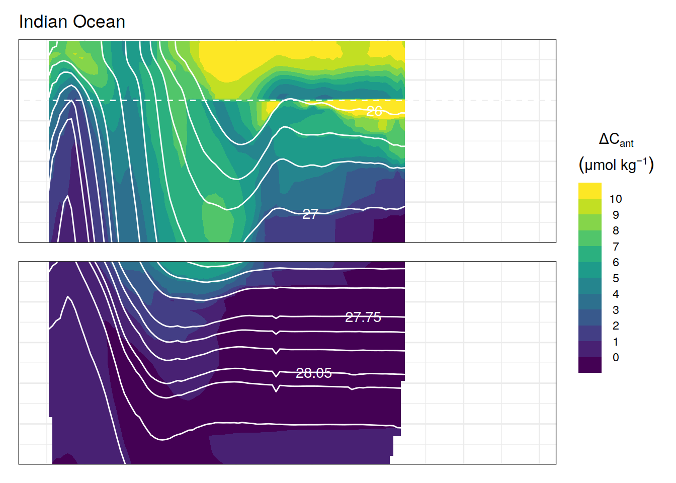
section_combined <-
section_combined_Atl | section_combined_Pac | section_combined_Ind

section_combined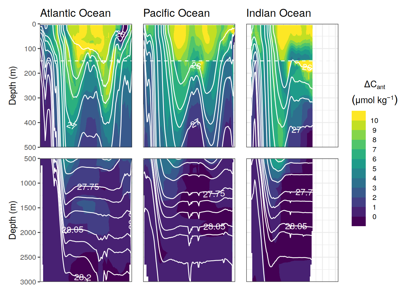
| Version | Author | Date |
|---|---|---|
| 0a9f7a7 | jens-daniel-mueller | 2021-04-22 |
3.3.2 Bias
breaks <- c(-Inf, seq(-6, 6, 2), Inf)
breaks_n <- length(breaks) - 1

legend_title = expression(atop(Delta * C[ant]~bias,
                               (mu * mol ~ kg ^ {
                                 -1
                               })))

cant_zonal_bias <- cant_zonal %>%
  filter(data_source %in% c("mod", "mod_truth")) %>%
  select(lat, depth, basin_AIP, data_source, cant_mean) %>%
  pivot_wider(names_from = data_source,
              values_from = cant_mean) %>%
  mutate(cant_bias = mod - mod_truth)

cant_zonal_bias <- full_join(
  cant_zonal_bias,
  cant_zonal_mod_truth %>% select(lat, depth, basin_AIP, gamma_mean)
)


i_basin_AIP <- "Atlantic"
slab_breaks <- params_local$slabs_Atl

# plot base section
section <-
  cant_zonal_bias %>%
  filter(basin_AIP == i_basin_AIP) %>%
  ggplot() +
  guides(fill = FALSE) +
  scale_y_reverse() +
  scale_x_continuous(breaks = seq(-100, 100, 20),
                     limits = c(min(cant_zonal$lat), max(cant_zonal$lat))) +
  geom_contour_filled(aes(lat, depth, z = cant_bias),
                      breaks = breaks) +
  scale_fill_brewer(
    palette = "RdBu",
    direction = -1,
    drop = FALSE,
    name = legend_title,
    guide = guide_colorsteps(barheight = unit(5, "cm"))
  ) +
  geom_contour(aes(lat, depth, z = gamma_mean),
               breaks = slab_breaks,
               col = "black") +
  geom_text_contour(
    aes(lat, depth, z = gamma_mean),
    breaks = slab_breaks,
    col = "black",
    skip = 2
  )

# cut surface water section
surface <-
  section +
  coord_cartesian(expand = 0,
                  ylim = c(500, 0)) +
  labs(y = "Depth (m)") +
  theme(
    axis.title.x = element_blank(),
    axis.text.x = element_blank(),
    axis.ticks.x = element_blank()
  )

# cut deep water section
deep <-
  section +
  coord_cartesian(expand = 0,
                  ylim = c(params_global$inventory_depth_standard, 500)) +
  labs(x = expression(latitude ~ (degree * N)), y = "Depth (m)")


# combine surface and deep water section
section_combined_Atl <-
  surface / deep +
  plot_layout(guides = "collect")

section_combined_Atl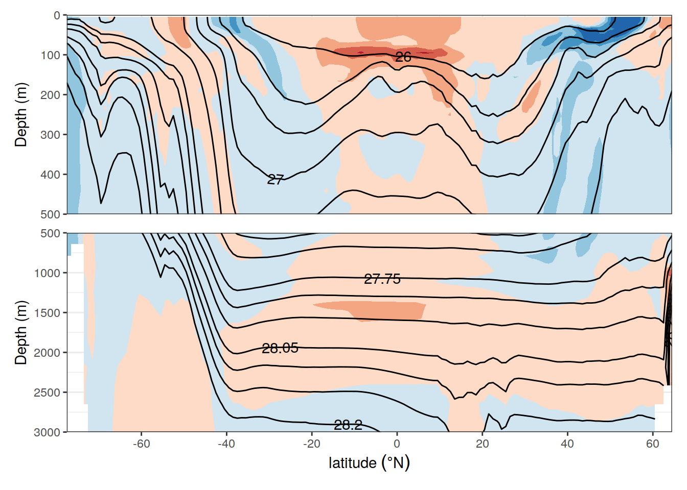
i_basin_AIP <- "Pacific"
slab_breaks <- params_local$slabs_Ind_Pac

# plot base section
section <-
  cant_zonal_bias %>%
  filter(basin_AIP == i_basin_AIP) %>%
  ggplot() +
  guides(fill = FALSE) +
  scale_y_reverse() +
  scale_x_continuous(breaks = seq(-100, 100, 20),
                     limits = c(min(cant_zonal$lat), max(cant_zonal$lat))) +
  geom_contour_filled(aes(lat, depth, z = cant_bias),
                      breaks = breaks) +
    scale_fill_brewer(
    palette = "RdBu",
    direction = -1,
    drop = FALSE,
    name = legend_title,
    guide = guide_colorsteps(barheight = unit(4, "cm"))
  ) +
  geom_hline(yintercept = params_local$depth_min,
             col = "black",
             linetype = 2) +
  geom_contour(aes(lat, depth, z = gamma_mean),
               breaks = slab_breaks,
               col = "black") +
  geom_text_contour(
    aes(lat, depth, z = gamma_mean),
    breaks = slab_breaks,
    col = "white",
    skip = 2
  )

# cut surface water section
surface <-
  section +
  coord_cartesian(expand = 0,
                  ylim = c(500, 0)) +
  labs(y = "Depth (m)") +
  theme(
    axis.title = element_blank(),
    axis.text = element_blank(),
    axis.ticks = element_blank()
  )

# cut deep water section
deep <-
  section +
  coord_cartesian(expand = 0,
                  ylim = c(params_global$inventory_depth_standard, 500)) +
  labs(x = expression(latitude ~ (degree * N)), y = "Depth (m)") +
  theme(
    axis.title.y = element_blank(),
    axis.text.y = element_blank(),
    axis.ticks.y = element_blank()
  )


# combine surface and deep water section
section_combined_Pac <-
  surface / deep +
  plot_layout(guides = "collect")

section_combined_Pac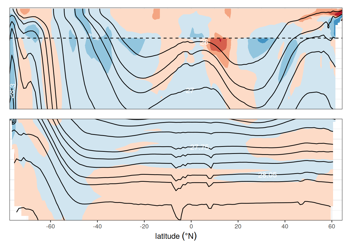
i_basin_AIP <- "Indian"
slab_breaks <- params_local$slabs_Ind_Pac

# plot base section
section <-
  cant_zonal_bias %>%
  filter(basin_AIP == i_basin_AIP) %>%
  ggplot() +
  guides(fill = guide_colorsteps(barheight = unit(6, "cm"))) +
  scale_y_reverse() +
  scale_x_continuous(breaks = seq(-100, 100, 20),
                     limits = c(min(cant_zonal$lat), max(cant_zonal$lat))) +
  geom_contour_filled(aes(lat, depth, z = cant_bias),
                      breaks = breaks) +
    scale_fill_brewer(
    palette = "RdBu",
    direction = -1,
    drop = FALSE,
    name = legend_title,
    guide = guide_colorsteps(barheight = unit(4, "cm"))
  ) +
  geom_hline(yintercept = params_local$depth_min,
             col = "white",
             linetype = 2) +
  geom_contour(aes(lat, depth, z = gamma_mean),
               breaks = slab_breaks,
               col = "black") +
  geom_text_contour(
    aes(lat, depth, z = gamma_mean),
    breaks = slab_breaks,
    col = "black",
    skip = 2
  )

# cut surface water section
surface <-
  section +
  coord_cartesian(expand = 0,
                  ylim = c(500, 0)) +
  labs(y = "Depth (m)") +
  theme(
    axis.title = element_blank(),
    axis.text = element_blank(),
    axis.ticks = element_blank()
  )

# cut deep water section
deep <-
  section +
  coord_cartesian(expand = 0,
                  ylim = c(params_global$inventory_depth_standard, 500)) +
  labs(x = expression(latitude ~ (degree * N)), y = "Depth (m)") +
  theme(
    axis.title.y = element_blank(),
    axis.text.y = element_blank(),
    axis.ticks.y = element_blank()
  )


# combine surface and deep water section
section_combined_Ind <-
  surface / deep +
  plot_layout(guides = "collect")

section_combined_Ind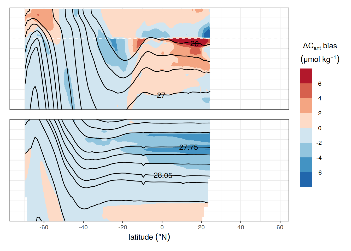
section_combined_bias <-
section_combined_Atl | section_combined_Pac | section_combined_Ind

section_mod_bias <-
section_combined / section_combined_bias


ggsave(plot = section_mod_bias,
       path = "output/publication",
       filename = "zonal_mean_section_mod_bias.png",
       height = 7,
       width = 14)
sessionInfo()R version 4.0.3 (2020-10-10)
Platform: x86_64-pc-linux-gnu (64-bit)
Running under: openSUSE Leap 15.2
Matrix products: default
BLAS: /usr/local/R-4.0.3/lib64/R/lib/libRblas.so
LAPACK: /usr/local/R-4.0.3/lib64/R/lib/libRlapack.so
locale:
[1] LC_CTYPE=en_US.UTF-8 LC_NUMERIC=C
[3] LC_TIME=en_US.UTF-8 LC_COLLATE=en_US.UTF-8
[5] LC_MONETARY=en_US.UTF-8 LC_MESSAGES=en_US.UTF-8
[7] LC_PAPER=en_US.UTF-8 LC_NAME=C
[9] LC_ADDRESS=C LC_TELEPHONE=C
[11] LC_MEASUREMENT=en_US.UTF-8 LC_IDENTIFICATION=C
attached base packages:
[1] stats graphics grDevices utils datasets methods base
other attached packages:
[1] marelac_2.1.10 shape_1.4.5 ggnewscale_0.4.5
[4] rnaturalearth_0.1.0 sf_0.9-8 metR_0.9.0
[7] scico_1.2.0 patchwork_1.1.1 collapse_1.5.0
[10] forcats_0.5.0 stringr_1.4.0 dplyr_1.0.5
[13] purrr_0.3.4 readr_1.4.0 tidyr_1.1.2
[16] tibble_3.0.4 ggplot2_3.3.3 tidyverse_1.3.0
[19] workflowr_1.6.2
loaded via a namespace (and not attached):
[1] fs_1.5.0 lubridate_1.7.9 gsw_1.0-5
[4] RColorBrewer_1.1-2 httr_1.4.2 rprojroot_2.0.2
[7] tools_4.0.3 backports_1.1.10 utf8_1.1.4
[10] R6_2.5.0 KernSmooth_2.23-17 rgeos_0.5-5
[13] DBI_1.1.0 colorspace_1.4-1 withr_2.3.0
[16] sp_1.4-4 rnaturalearthdata_0.1.0 tidyselect_1.1.0
[19] compiler_4.0.3 git2r_0.27.1 cli_2.1.0
[22] rvest_0.3.6 xml2_1.3.2 isoband_0.2.2
[25] labeling_0.4.2 scales_1.1.1 checkmate_2.0.0
[28] classInt_0.4-3 digest_0.6.27 rmarkdown_2.5
[31] oce_1.2-0 pkgconfig_2.0.3 htmltools_0.5.0
[34] dbplyr_1.4.4 rlang_0.4.10 readxl_1.3.1
[37] rstudioapi_0.11 farver_2.0.3 generics_0.0.2
[40] jsonlite_1.7.1 magrittr_1.5 Matrix_1.2-18
[43] Rcpp_1.0.5 munsell_0.5.0 fansi_0.4.1
[46] lifecycle_1.0.0 stringi_1.5.3 whisker_0.4
[49] yaml_2.2.1 plyr_1.8.6 grid_4.0.3
[52] blob_1.2.1 parallel_4.0.3 promises_1.1.1
[55] crayon_1.3.4 lattice_0.20-41 haven_2.3.1
[58] hms_0.5.3 seacarb_3.2.14 knitr_1.30
[61] pillar_1.4.7 reprex_0.3.0 glue_1.4.2
[64] evaluate_0.14 RcppArmadillo_0.10.1.2.0 data.table_1.13.2
[67] modelr_0.1.8 vctrs_0.3.5 httpuv_1.5.4
[70] testthat_2.3.2 cellranger_1.1.0 gtable_0.3.0
[73] assertthat_0.2.1 xfun_0.18 broom_0.7.5
[76] RcppEigen_0.3.3.7.0 e1071_1.7-4 later_1.1.0.1
[79] viridisLite_0.3.0 class_7.3-17 memoise_1.1.0
[82] units_0.6-7 ellipsis_0.3.1