Results publication
Jens Daniel Müller
02 February, 2022
Last updated: 2022-02-02
Checks: 7 0
Knit directory: emlr_obs_analysis/analysis/
This reproducible R Markdown analysis was created with workflowr (version 1.7.0). The Checks tab describes the reproducibility checks that were applied when the results were created. The Past versions tab lists the development history.
Great! Since the R Markdown file has been committed to the Git repository, you know the exact version of the code that produced these results.
Great job! The global environment was empty. Objects defined in the global environment can affect the analysis in your R Markdown file in unknown ways. For reproduciblity it’s best to always run the code in an empty environment.
The command set.seed(20210412) was run prior to running the code in the R Markdown file. Setting a seed ensures that any results that rely on randomness, e.g. subsampling or permutations, are reproducible.
Great job! Recording the operating system, R version, and package versions is critical for reproducibility.
Nice! There were no cached chunks for this analysis, so you can be confident that you successfully produced the results during this run.
Great job! Using relative paths to the files within your workflowr project makes it easier to run your code on other machines.
Great! You are using Git for version control. Tracking code development and connecting the code version to the results is critical for reproducibility.
The results in this page were generated with repository version 9d11695. See the Past versions tab to see a history of the changes made to the R Markdown and HTML files.
Note that you need to be careful to ensure that all relevant files for the analysis have been committed to Git prior to generating the results (you can use wflow_publish or wflow_git_commit). workflowr only checks the R Markdown file, but you know if there are other scripts or data files that it depends on. Below is the status of the Git repository when the results were generated:
Ignored files:
    Ignored:    .Rhistory
    Ignored:    .Rproj.user/
    Ignored:    data/
    Ignored:    output/other/
    Ignored:    output/publication/
Note that any generated files, e.g. HTML, png, CSS, etc., are not included in this status report because it is ok for generated content to have uncommitted changes.
These are the previous versions of the repository in which changes were made to the R Markdown (analysis/results_publication.Rmd) and HTML (docs/results_publication.html) files. If you’ve configured a remote Git repository (see ?wflow_git_remote), click on the hyperlinks in the table below to view the files as they were in that past version.
| File | Version | Author | Date | Message |
|---|---|---|---|---|
| Rmd | 9d11695 | jens-daniel-mueller | 2022-02-02 | scaled budget to atm pco2 increase |
| html | 32e9682 | jens-daniel-mueller | 2022-02-02 | Build site. |
| Rmd | 5cc5572 | jens-daniel-mueller | 2022-02-02 | included Sabine column inventory as reference |
| html | 913e42f | jens-daniel-mueller | 2022-02-01 | Build site. |
| Rmd | c4b2de9 | jens-daniel-mueller | 2022-02-01 | updated profile plots |
| html | 189de95 | jens-daniel-mueller | 2022-02-01 | Build site. |
| Rmd | b0c17bc | jens-daniel-mueller | 2022-02-01 | updated profile plots |
| html | ab001eb | jens-daniel-mueller | 2022-01-31 | Build site. |
| Rmd | ccf6723 | jens-daniel-mueller | 2022-01-31 | filled step plot for layer budgets |
| html | d2ae5fe | jens-daniel-mueller | 2022-01-31 | Build site. |
| Rmd | 278523c | jens-daniel-mueller | 2022-01-31 | step plot for layer budgets |
| html | b62308d | jens-daniel-mueller | 2022-01-31 | Build site. |
| Rmd | 714c5cc | jens-daniel-mueller | 2022-01-31 | step plot for layer budgets |
| html | ec7fe7e | jens-daniel-mueller | 2022-01-31 | Build site. |
| Rmd | 5c948ae | jens-daniel-mueller | 2022-01-31 | added time series vs atm pco2 |
| html | de557de | jens-daniel-mueller | 2022-01-28 | Build site. |
| html | 5f2aed0 | jens-daniel-mueller | 2022-01-27 | Build site. |
| Rmd | 54c9e26 | jens-daniel-mueller | 2022-01-27 | added layer budget profiles |
| html | eccd82b | jens-daniel-mueller | 2022-01-26 | Build site. |
| Rmd | c5577d3 | jens-daniel-mueller | 2022-01-26 | added meand sd to offset mean concentrations profiles |
| html | c6fe495 | jens-daniel-mueller | 2022-01-26 | Build site. |
| Rmd | e0e7974 | jens-daniel-mueller | 2022-01-26 | added offset mean concentrations profiles |
| html | 9753eb8 | jens-daniel-mueller | 2022-01-26 | Build site. |
| html | b1d7720 | jens-daniel-mueller | 2022-01-21 | Build site. |
| Rmd | 0210ed5 | jens-daniel-mueller | 2022-01-21 | added mean concentrations profiles per 5 basins |
| html | d6b399a | jens-daniel-mueller | 2022-01-21 | Build site. |
| Rmd | da17a07 | jens-daniel-mueller | 2022-01-21 | added mean concentrations profiles |
| html | c499be8 | jens-daniel-mueller | 2022-01-21 | Build site. |
| Rmd | d941871 | jens-daniel-mueller | 2022-01-21 | run color map test |
| html | e572075 | jens-daniel-mueller | 2022-01-21 | Build site. |
| Rmd | 99b6c92 | jens-daniel-mueller | 2022-01-21 | run color map test |
| html | 4fe7150 | jens-daniel-mueller | 2022-01-21 | Build site. |
| Rmd | 0379e99 | jens-daniel-mueller | 2022-01-21 | script cleaning |
| html | 49b41cf | jens-daniel-mueller | 2022-01-21 | Build site. |
| Rmd | 2c82651 | jens-daniel-mueller | 2022-01-21 | added map of scaled absolute change |
| html | c0807e8 | jens-daniel-mueller | 2022-01-21 | Build site. |
| Rmd | 5dd3d7a | jens-daniel-mueller | 2022-01-21 | added map of scaled relative change |
| html | 22b421f | jens-daniel-mueller | 2022-01-21 | Build site. |
| Rmd | 2c3fa75 | jens-daniel-mueller | 2022-01-21 | cleaned alluvial plots |
| html | 1a35f1f | jens-daniel-mueller | 2022-01-20 | Build site. |
| Rmd | e58f510 | jens-daniel-mueller | 2022-01-20 | added relative changes to alluvial plots |
| html | b503ae1 | jens-daniel-mueller | 2022-01-20 | Build site. |
| Rmd | 2eb2567 | jens-daniel-mueller | 2022-01-20 | added relative changes to alluvial plots |
| html | cc31f4b | jens-daniel-mueller | 2022-01-20 | Build site. |
| Rmd | 416e107 | jens-daniel-mueller | 2022-01-20 | added delta dcant map |
| html | 11a800b | jens-daniel-mueller | 2022-01-20 | Build site. |
| Rmd | 81a40d5 | jens-daniel-mueller | 2022-01-20 | updated alluvial plots |
| html | 3087804 | jens-daniel-mueller | 2022-01-20 | Build site. |
| Rmd | 2ae5966 | jens-daniel-mueller | 2022-01-20 | updated alluvial plots |
| html | 6d566d5 | jens-daniel-mueller | 2022-01-20 | Build site. |
| Rmd | 4901b0f | jens-daniel-mueller | 2022-01-20 | updated alluvial plots |
| html | 44796b1 | jens-daniel-mueller | 2022-01-20 | Build site. |
| Rmd | cdbd92c | jens-daniel-mueller | 2022-01-20 | created alluvial plots |
| html | 48ec4c6 | jens-daniel-mueller | 2022-01-19 | Build site. |
| Rmd | 0fb2ae5 | jens-daniel-mueller | 2022-01-19 | printed column inv from AIP standard runs |
| html | f347cd7 | jens-daniel-mueller | 2022-01-18 | Build site. |
| Rmd | 86b711c | jens-daniel-mueller | 2022-01-18 | plot hemisphere budgets and publication results |
1 Libraries
2 Read files
2.1 Paths and Versions
version_id_pattern <- "103"

# identify required version IDs

Version_IDs_1 <- list.files(path = "/nfs/kryo/work/jenmueller/emlr_cant/observations",
                            pattern = paste0("v_1", version_id_pattern))

Version_IDs_2 <- list.files(path = "/nfs/kryo/work/jenmueller/emlr_cant/observations",
                            pattern = paste0("v_2", version_id_pattern))

Version_IDs_3 <- list.files(path = "/nfs/kryo/work/jenmueller/emlr_cant/observations",
                            pattern = paste0("v_3", version_id_pattern))

Version_IDs <- c(Version_IDs_1, Version_IDs_2, Version_IDs_3)

print(Version_IDs)
[1] "v_1103" "v_2103" "v_3103"2.2 Parameters
for (i_Version_IDs in Version_IDs) {
  path_version_data     <-
    paste(path_observations,
          i_Version_IDs,
          "/data/",
          sep = "")

  params_local <-
    read_rds(paste(path_version_data,
                   "params_local.rds",
                   sep = ""))

  params_local <- bind_cols(
    Version_ID = i_Version_IDs,
    tref1 = params_local$tref1,
    tref2 = params_local$tref2
  )

  tref <- read_csv(paste(path_version_data,
                         "tref.csv",
                         sep = ""))

  params_local <- params_local %>%
    mutate(
      median_year_1 = sort(tref$median_year)[1],
      median_year_2 = sort(tref$median_year)[2],
      duration = median_year_2 - median_year_1,
      period = paste(median_year_1, "-", median_year_2)
    )
  if (exists("params_local_all")) {
    params_local_all <- bind_rows(params_local_all, params_local)
  }

  if (!exists("params_local_all")) {
    params_local_all <- params_local
  }


}

rm(params_local,
   tref)

params_local_all <- params_local_all %>%
  select(Version_ID, period, tref1, tref2)
2.3 Budgets
for (i_Version_IDs in Version_IDs) {
  # i_Version_IDs <- Version_IDs[1]

  path_version_data     <-
    paste(path_observations,
          i_Version_IDs,
          "/data/",
          sep = "")

  # load and join data files

  dcant_budget_global <-
    read_csv(paste(path_version_data,
                   "dcant_budget_global.csv",
                   sep = ""))

  dcant_budget_global_mod_truth <-
    read_csv(paste(
      path_version_data,
      "dcant_budget_global_mod_truth.csv",
      sep = ""
    ))
  #
  # dcant_budget_global_bias <-
  #   read_csv(paste(path_version_data,
  #                  "dcant_budget_global_bias.csv",
  #                  sep = ""))
  #
  # lm_best_predictor_counts <-
  #   read_csv(paste(path_version_data,
  #                  "lm_best_predictor_counts.csv",
  #                  sep = ""))
  #
  # lm_best_dcant <-
  #   read_csv(paste(path_version_data,
  #                  "lm_best_dcant.csv",
  #                  sep = ""))

  dcant_budget_global <- bind_rows(dcant_budget_global,
                                      dcant_budget_global_mod_truth)

  dcant_budget_global <- dcant_budget_global %>%
    mutate(Version_ID = i_Version_IDs)

  # dcant_budget_global_bias <- dcant_budget_global_bias %>%
  #   mutate(Version_ID = i_Version_IDs)
  #
  # lm_best_predictor_counts <- lm_best_predictor_counts %>%
  #   mutate(Version_ID = i_Version_IDs)
  #
  # lm_best_dcant <- lm_best_dcant %>%
  #   mutate(Version_ID = i_Version_IDs)

  if (exists("dcant_budget_global_all")) {
    dcant_budget_global_all <-
      bind_rows(dcant_budget_global_all, dcant_budget_global)
  }

  if (!exists("dcant_budget_global_all")) {
    dcant_budget_global_all <- dcant_budget_global
  }

  # if (exists("dcant_budget_global_bias_all")) {
  #   dcant_budget_global_bias_all <-
  #     bind_rows(dcant_budget_global_bias_all,
  #               dcant_budget_global_bias)
  # }
  #
  # if (!exists("dcant_budget_global_bias_all")) {
  #   dcant_budget_global_bias_all <- dcant_budget_global_bias
  # }
  #
  #
  # if (exists("lm_best_predictor_counts_all")) {
  #   lm_best_predictor_counts_all <-
  #     bind_rows(lm_best_predictor_counts_all, lm_best_predictor_counts)
  # }
  #
  # if (!exists("lm_best_predictor_counts_all")) {
  #   lm_best_predictor_counts_all <- lm_best_predictor_counts
  # }
  #
  # if (exists("lm_best_dcant_all")) {
  #   lm_best_dcant_all <-
  #     bind_rows(lm_best_dcant_all, lm_best_dcant)
  # }
  #
  # if (!exists("lm_best_dcant_all")) {
  #   lm_best_dcant_all <- lm_best_dcant
  # }
  #
  # if (exists("params_local_all")) {
  #   params_local_all <- bind_rows(params_local_all, params_local)
  # }
  #
  # if (!exists("params_local_all")) {
  #   params_local_all <- params_local
  # }
  #

}

rm(
  dcant_budget_global,
  # dcant_budget_global_bias,
  dcant_budget_global_mod_truth
  # lm_best_predictor_counts,
  # lm_best_dcant
)
for (i_Version_IDs in Version_IDs) {
# i_Version_IDs <- Version_IDs[1]
print(i_Version_IDs)
path_version_data <-
paste(path_observations,
i_Version_IDs,
"/data/",
sep = "")
# load and join data files
dcant_budget_basin_MLR <-
read_csv(paste(path_version_data,
"dcant_budget_basin_MLR.csv",
sep = ""))
dcant_budget_basin_MLR_mod_truth <-
read_csv(paste(
path_version_data,
"dcant_budget_basin_MLR_mod_truth.csv",
sep = ""
))
dcant_budget_basin_MLR <- bind_rows(dcant_budget_basin_MLR,
dcant_budget_basin_MLR_mod_truth)
dcant_budget_basin_MLR <- dcant_budget_basin_MLR %>%
mutate(Version_ID = i_Version_IDs)
if (exists("dcant_budget_basin_MLR_all")) {
dcant_budget_basin_MLR_all <-
bind_rows(dcant_budget_basin_MLR_all, dcant_budget_basin_MLR)
}
if (!exists("dcant_budget_basin_MLR_all")) {
dcant_budget_basin_MLR_all <- dcant_budget_basin_MLR
}
}[1] "v_1103"
[1] "v_2103"
[1] "v_3103"rm(
dcant_budget_basin_MLR,
dcant_budget_basin_MLR_mod_truth
)dcant_budget_global_all <- dcant_budget_global_all %>%
filter(estimate == "dcant",
method == "total") %>%
select(-c(estimate, method)) %>%
rename(dcant = value)
# dcant_budget_global_all_depth <- dcant_budget_global_all
dcant_budget_global_all <- dcant_budget_global_all %>%
filter(inv_depth == params_global$inventory_depth_standard)
# dcant_budget_global_bias_all <- dcant_budget_global_bias_all %>%
# filter(estimate == "dcant") %>%
# select(-c(estimate))
# dcant_budget_global_bias_all_depth <- dcant_budget_global_bias_all
#
# dcant_budget_global_bias_all <- dcant_budget_global_bias_all %>%
# filter(inv_depth == params_global$inventory_depth_standard)dcant_budget_basin_MLR_all <- dcant_budget_basin_MLR_all %>%
filter(estimate == "dcant",
method == "total") %>%
select(-c(estimate, method)) %>%
rename(dcant = value)
dcant_budget_basin_MLR_all <- dcant_budget_basin_MLR_all %>%
filter(inv_depth == params_global$inventory_depth_standard)2.4 Inventories
for (i_Version_IDs in Version_IDs) {
  # i_Version_IDs <- Version_IDs[1]

  path_version_data     <-
    paste(path_observations,
          i_Version_IDs,
          "/data/",
          sep = "")

  # load and join data files

  dcant_inv <-
    read_csv(paste(path_version_data,
                   "dcant_inv.csv",
                   sep = ""))

  dcant_inv_mod_truth <-
    read_csv(paste(path_version_data,
                   "dcant_inv_mod_truth.csv",
                   sep = "")) %>%
    filter(method == "total") %>%
    select(-method)

  dcant_inv_bias <-
    read_csv(paste(path_version_data,
                   "dcant_inv_bias.csv",
                   sep = "")) %>%
    mutate(Version_ID = i_Version_IDs)

  dcant_inv <- bind_rows(dcant_inv,
                         dcant_inv_mod_truth) %>%
    mutate(Version_ID = i_Version_IDs)

  dcant_budget_lat_grid <-
    read_csv(paste(path_version_data,
                   "dcant_budget_lat_grid.csv",
                   sep = "")) %>%
    mutate(Version_ID = i_Version_IDs)

  dcant_budget_lon_grid <-
    read_csv(paste(path_version_data,
                   "dcant_budget_lon_grid.csv",
                   sep = "")) %>%
    mutate(Version_ID = i_Version_IDs)
  if (exists("dcant_inv_all")) {
    dcant_inv_all <- bind_rows(dcant_inv_all, dcant_inv)
  }

  if (!exists("dcant_inv_all")) {
    dcant_inv_all <- dcant_inv
  }

  if (exists("dcant_inv_bias_all")) {
    dcant_inv_bias_all <- bind_rows(dcant_inv_bias_all, dcant_inv_bias)
  }

  if (!exists("dcant_inv_bias_all")) {
    dcant_inv_bias_all <- dcant_inv_bias
  }

  if (exists("dcant_budget_lat_grid_all")) {
    dcant_budget_lat_grid_all <- bind_rows(dcant_budget_lat_grid_all, dcant_budget_lat_grid)
  }

  if (!exists("dcant_budget_lat_grid_all")) {
    dcant_budget_lat_grid_all <- dcant_budget_lat_grid
  }

  if (exists("dcant_budget_lon_grid_all")) {
    dcant_budget_lon_grid_all <- bind_rows(dcant_budget_lon_grid_all, dcant_budget_lon_grid)
  }

  if (!exists("dcant_budget_lon_grid_all")) {
    dcant_budget_lon_grid_all <- dcant_budget_lon_grid
  }
}

rm(dcant_inv,
   dcant_inv_bias,
   dcant_inv_mod_truth,
   dcant_budget_lat_grid,
   dcant_budget_lon_grid)
dcant_inv_all <- dcant_inv_all %>%
filter(inv_depth == params_global$inventory_depth_standard)
dcant_budget_lat_grid_all <- dcant_budget_lat_grid_all %>%
filter(inv_depth == params_global$inventory_depth_standard)
dcant_budget_lon_grid_all <- dcant_budget_lon_grid_all %>%
filter(inv_depth == params_global$inventory_depth_standard)dcant_budget_lat_grid_all <- dcant_budget_lat_grid_all %>%
pivot_wider(names_from = estimate,
values_from = value) %>%
filter(period != "1994 - 2014",
method == "total")
dcant_budget_lon_grid_all <- dcant_budget_lon_grid_all %>%
pivot_wider(names_from = estimate,
values_from = value) %>%
filter(period != "1994 - 2014",
method == "total")2.5 Zonal sections
for (i_Version_IDs in Version_IDs) {

  path_version_data     <-
  paste(path_observations,
        i_Version_IDs,
        "/data/",
        sep = "")

  # load and join data files

  dcant_zonal <-
    read_csv(paste(path_version_data,
                   "dcant_zonal.csv",
                   sep = ""))

  dcant_zonal_mod_truth <-
    read_csv(paste(path_version_data,
                   "dcant_zonal_mod_truth.csv",
                   sep = ""))

  dcant_zonal <- bind_rows(dcant_zonal,
                         dcant_zonal_mod_truth)

  dcant_profile <-
    read_csv(paste(path_version_data,
                   "dcant_profile.csv",
                   sep = ""))

  dcant_profile_mod_truth <-
    read_csv(paste(path_version_data,
                   "dcant_profile_mod_truth.csv",
                   sep = ""))


  dcant_profile_basin_MLR <-
    read_csv(paste(path_version_data,
                   "dcant_profile_basin_MLR.csv",
                   sep = ""))

  dcant_profile <- bind_rows(dcant_profile,
                             dcant_profile_mod_truth)

  dcant_budget_basin_AIP_layer <-
    read_csv(paste(path_version_data,
                   "dcant_budget_basin_AIP_layer.csv",
                   sep = ""))

  dcant_budget_basin_MLR_layer <-
    read_csv(paste(path_version_data,
                   "dcant_budget_basin_MLR_layer.csv",
                   sep = ""))

  dcant_zonal_bias <-
    read_csv(paste(path_version_data,
                   "dcant_zonal_bias.csv",
                   sep = ""))


  dcant_zonal <- dcant_zonal %>%
    mutate(Version_ID = i_Version_IDs)

  dcant_profile <- dcant_profile %>%
    mutate(Version_ID = i_Version_IDs)

  dcant_profile_basin_MLR <- dcant_profile_basin_MLR %>%
    mutate(Version_ID = i_Version_IDs)

  dcant_budget_basin_AIP_layer <- dcant_budget_basin_AIP_layer %>%
    mutate(Version_ID = i_Version_IDs)

  dcant_budget_basin_MLR_layer <- dcant_budget_basin_MLR_layer %>%
    mutate(Version_ID = i_Version_IDs)

  dcant_zonal_bias <- dcant_zonal_bias %>%
    mutate(Version_ID = i_Version_IDs)


  if (exists("dcant_zonal_all")) {
    dcant_zonal_all <- bind_rows(dcant_zonal_all, dcant_zonal)
  }

  if (!exists("dcant_zonal_all")) {
    dcant_zonal_all <- dcant_zonal
  }

  if (exists("dcant_profile_all")) {
    dcant_profile_all <- bind_rows(dcant_profile_all, dcant_profile)
  }

  if (!exists("dcant_profile_all")) {
    dcant_profile_all <- dcant_profile
  }

  if (exists("dcant_profile_basin_MLR_all")) {
    dcant_profile_basin_MLR_all <- bind_rows(dcant_profile_basin_MLR_all, dcant_profile_basin_MLR)
  }

  if (!exists("dcant_profile_basin_MLR_all")) {
    dcant_profile_basin_MLR_all <- dcant_profile_basin_MLR
  }

  if (exists("dcant_budget_basin_AIP_layer_all")) {
    dcant_budget_basin_AIP_layer_all <-
      bind_rows(dcant_budget_basin_AIP_layer_all,
                dcant_budget_basin_AIP_layer)
  }

  if (!exists("dcant_budget_basin_AIP_layer_all")) {
    dcant_budget_basin_AIP_layer_all <- dcant_budget_basin_AIP_layer
  }

  if (exists("dcant_budget_basin_MLR_layer_all")) {
    dcant_budget_basin_MLR_layer_all <-
      bind_rows(dcant_budget_basin_MLR_layer_all,
                dcant_budget_basin_MLR_layer)
  }

  if (!exists("dcant_budget_basin_MLR_layer_all")) {
    dcant_budget_basin_MLR_layer_all <- dcant_budget_basin_MLR_layer
  }

  if (exists("dcant_zonal_bias_all")) {
    dcant_zonal_bias_all <- bind_rows(dcant_zonal_bias_all, dcant_zonal_bias)
  }

  if (!exists("dcant_zonal_bias_all")) {
    dcant_zonal_bias_all <- dcant_zonal_bias
  }

}

rm(dcant_zonal, dcant_zonal_bias, dcant_zonal_mod_truth,
   dcant_budget_basin_AIP_layer, dcant_budget_basin_MLR_layer)
2.6 Atm CO2
co2_atm <-
  read_csv(paste(path_preprocessing,
                 "co2_atm.csv",
                 sep = ""))
2.7 Sabine total Cant
tcant_inv <-
  read_csv(paste(path_preprocessing,
                  "S04_tcant_inv.csv", sep = ""))

tcant_inv <- tcant_inv %>%
  filter(inv_depth == 3000) %>%
  rename(dcant = tcant,
         dcant_pos = tcant_pos) %>%
  mutate(tref1 = 1750,
         tref2 = 1994)
3 Define labels
dcant_pgc_label <- expression(Delta * C["ant"]~(PgC))
dcant_pgc_scaled_label <- expression(Delta * C["ant"]~(PgC~µatm^{-1}))

dcant_umol_label <- expression(Delta * C[ant]~(mu * mol ~ kg ^ {-1}))
ddcant_umol_label <- expression(Delta * Delta * C[ant]~(mu * mol ~ kg ^ {-1}))

dcant_layer_budget_label <-
  expression(Delta ~ C[ant] ~ "budget per 500m depth layer (PgC)")
4 Inventory maps
4.1 Absoulte values
4.1.1 dcant - absolute
dcant_inv_all <- dcant_inv_all %>%
  filter(data_source %in% c("obs"),
         period != "1994 - 2014")

dcant_inv_all <- left_join(dcant_inv_all,
                           co2_atm %>% rename(tref1 = year,
                                              pCO21 = pCO2))

dcant_inv_all <- left_join(dcant_inv_all,
                           co2_atm %>% rename(tref2 = year,
                                              pCO22 = pCO2))


tcant_inv <- tcant_inv %>%
  mutate(pCO21 = 280)

tcant_inv <- left_join(tcant_inv,
                       co2_atm %>% rename(tref2 = year,
                                          pCO22 = pCO2))

dcant_inv_all <- bind_rows(
  dcant_inv_all,
  tcant_inv %>% mutate(period = paste(tref1, tref2, sep = " - "))
)


dcant_inv_all <- dcant_inv_all %>%
  mutate(delta_pCO2 = pCO22 - pCO21,
         dcant_scaled = dcant / delta_pCO2,
         dcant_pos_scaled = dcant_pos / delta_pCO2) %>%
  select(-starts_with("pCO2"))

dcant_inv_all %>%
  p_map_cant_inv(var = "dcant") +
  facet_grid(period ~ .) +
  theme(axis.text = element_blank(),
        axis.ticks = element_blank())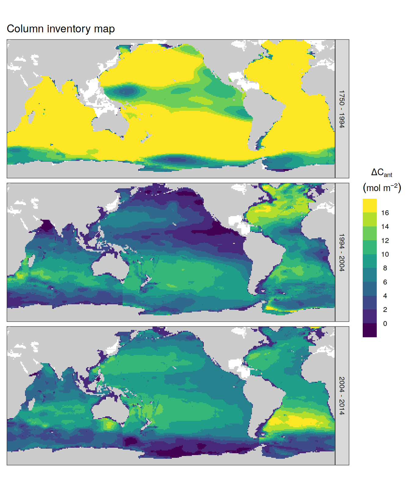
dcant_inv_all %>%
  p_map_cant_inv(var = "dcant_scaled",
                 breaks = c(-Inf, seq(0, 1, 0.1), Inf),) +
  facet_grid(period ~ .) +
  theme(axis.text = element_blank(),
        axis.ticks = element_blank())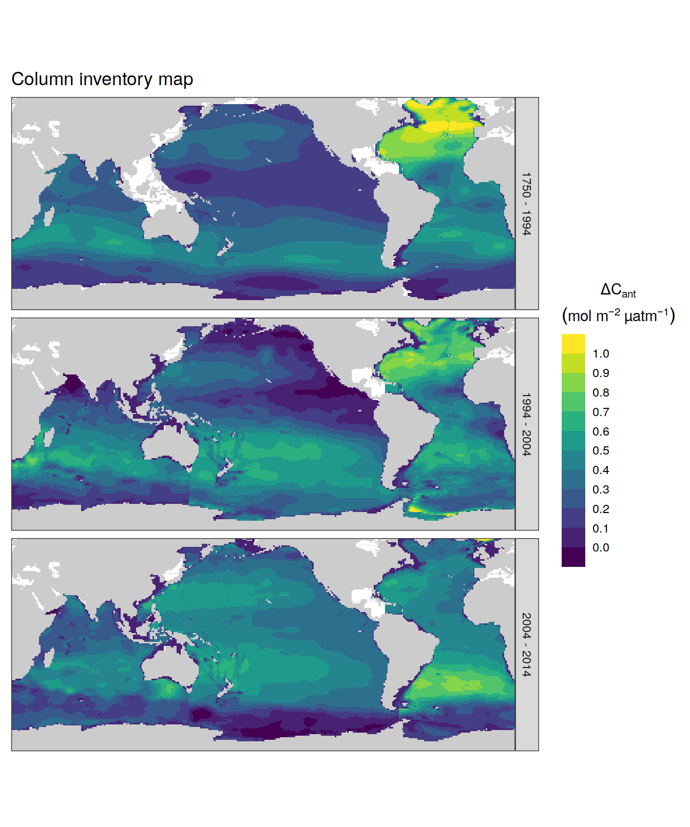
dcant_inv_all %>%
  p_map_cant_inv(var = "dcant_pos_scaled",
                 breaks = c(-Inf, seq(0, 1, 0.1), Inf),) +
  facet_grid(period ~ .) +
  theme(axis.text = element_blank(),
        axis.ticks = element_blank())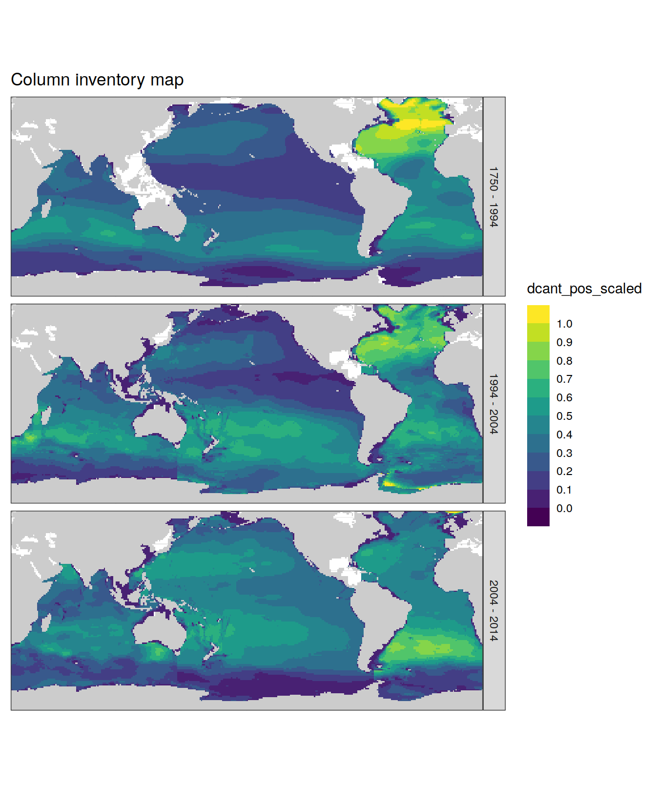
| Version | Author | Date |
|---|---|---|
| 32e9682 | jens-daniel-mueller | 2022-02-02 |
4.1.1.1 test color palettes
breaks <- c(-Inf, seq(0, 16, 2), Inf)

legend_title <- expression(atop(Delta * C["ant"],
                                (mol ~ m ^ {
                                  -2
                                })))

breaks_n <- length(breaks) - 1

dcant_inv_all_color_test <- dcant_inv_all %>%
  filter(data_source %in% c("obs"),
         period == "2004 - 2014") %>%
  mutate(dcant_int = cut(dcant,
                         breaks,
                         right = FALSE))

scico_continous_palettes <- c(
  "acton",
  "bamako",
  "batlow",
  "bilbao",
  "buda",
  "davos",
  "devon",
  "grayC",
  "hawaii",
  "imola",
  "lajolla",
  "lapaz",
  "nuuk",
  "oslo",
  "tokyo",
  "turku"
)


for (i_palette in scico_continous_palettes) {
  p_reg <- map +
    geom_tile(data = dcant_inv_all_color_test,
              aes(lon, lat, fill = dcant_int)) +
    scale_fill_scico_d(
      palette = i_palette,
      drop = FALSE,
      name = legend_title,
      guide = "none"
    ) +
    # guides(fill = guide_colorsteps(barheight = unit(3, "cm"))) +
    labs(title = i_palette)

  p_rev <- map +
    geom_tile(data = dcant_inv_all_color_test,
              aes(lon, lat, fill = dcant_int)) +
    scale_fill_scico_d(
      palette = i_palette,
      drop = FALSE,
      name = legend_title,
      direction = -1,
      guide = "none"
    ) +
    # guides(fill = guide_colorsteps(barheight = unit(3, "cm"))) +
    labs(title = paste(i_palette, "rev"))

  print(p_reg | p_rev)

}


viridis_continous_palettes <- c(
  "civides",
  "magma",
  "inferno",
  "plasma"
)


for (i_palette in viridis_continous_palettes) {
  p_reg <- map +
    geom_tile(data = dcant_inv_all_color_test,
              aes(lon, lat, fill = dcant_int)) +
    scale_fill_viridis_d(
      option = i_palette,
      drop = FALSE,
      name = legend_title,
      guide = "none"
    ) +
    # guides(fill = guide_colorsteps(barheight = unit(3, "cm"))) +
    labs(title = i_palette)

  p_rev <- map +
    geom_tile(data = dcant_inv_all_color_test,
              aes(lon, lat, fill = dcant_int)) +
    scale_fill_viridis_d(
      option = i_palette,
      drop = FALSE,
      name = legend_title,
      direction = -1,
      guide = "none"
    ) +
    # guides(fill = guide_colorsteps(barheight = unit(3, "cm"))) +
    labs(title = paste(i_palette, "rev"))

  print(p_reg | p_rev)

}
4.1.2 dcant - absolute delta
dcant_inv_all %>%
  filter(data_source %in% c("mod", "obs"),
         period != "1994 - 2014") %>%
  select(data_source, lon, lat, basin_AIP, period, dcant) %>%
  pivot_wider(names_from = period,
              values_from = dcant) %>%
  mutate(delta_dcant = `2004 - 2014` - `1994 - 2004`) %>%
  group_by(data_source) %>%
  group_split() %>%
  # head(1) %>%
  map(
    ~ p_map_cant_inv(df = .x,
                     var = "delta_dcant",
                     subtitle_text = paste("data_source:",
                                           unique(.x$data_source)),
                     col = "divergent") +
      # facet_grid(period ~ .) +
      theme(axis.text = element_blank(),
            axis.ticks = element_blank())
  )
[[1]]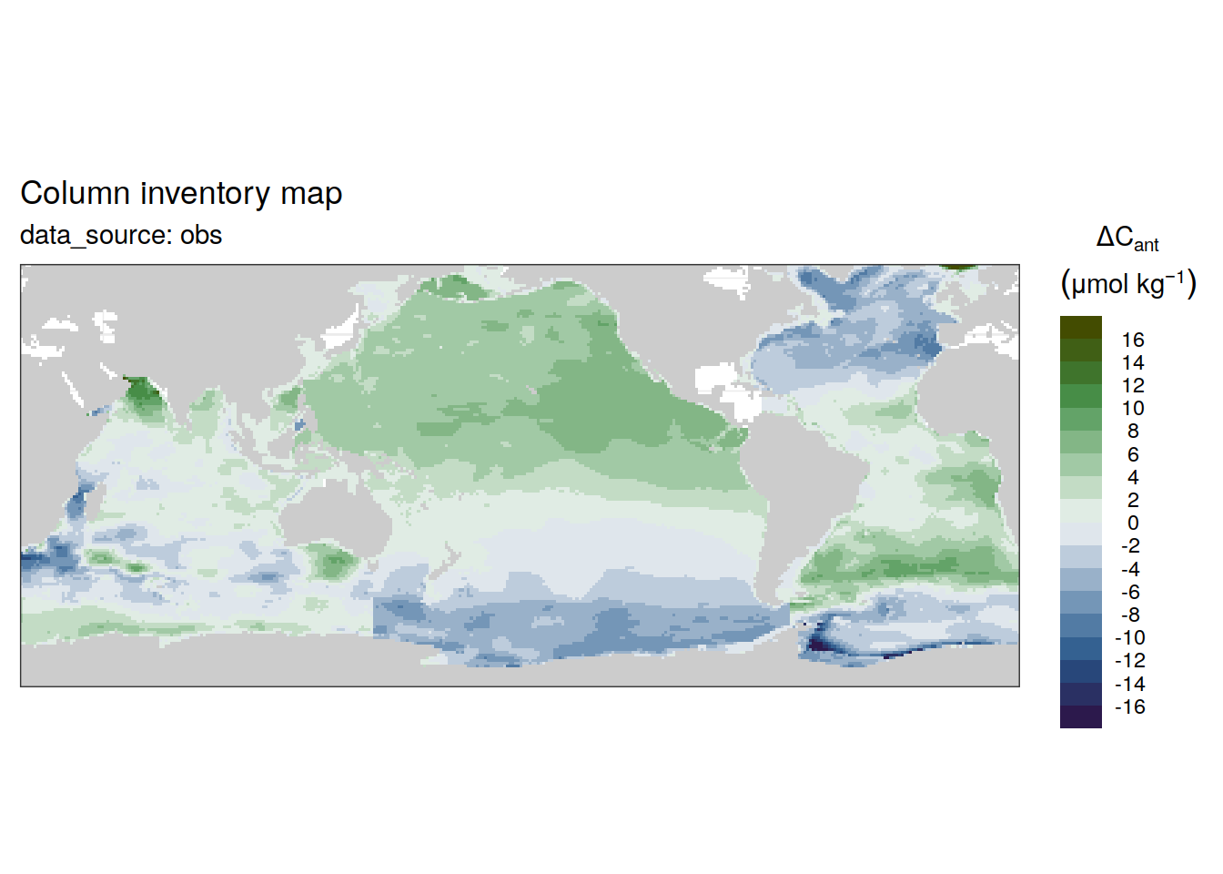
4.1.3 dcant - absolute delta scaled
dcant_budget_scaling <- dcant_budget_global_all %>%
  filter(#data_source %in% c("mod", "obs"),
         period != "1994 - 2014") %>%
  select(data_source, period, dcant) %>%
  pivot_wider(names_from = period,
              values_from = dcant) %>%
  mutate(dcant_scaling = `2004 - 2014` / `1994 - 2004`) %>%
  select(data_source, dcant_scaling)


left_join(dcant_inv_all,
          dcant_budget_scaling) %>%
  filter(#data_source %in% c("mod", "obs"),
         period != "1994 - 2014") %>%
  select(data_source, lon, lat, basin_AIP, period, dcant, dcant_scaling) %>%
  pivot_wider(names_from = period,
              values_from = dcant) %>%
  mutate(delta_dcant = `2004 - 2014` - `1994 - 2004`*dcant_scaling) %>%
  group_by(data_source) %>%
  group_split() %>%
  # head(1) %>%
  map(
    ~ p_map_cant_inv(df = .x,
                     var = "delta_dcant",
                     subtitle_text = paste("data_source:",
                                           unique(.x$data_source)),
                     col = "divergent") +
      # facet_grid(period ~ .) +
      theme(axis.text = element_blank(),
            axis.ticks = element_blank())
  )
[[1]]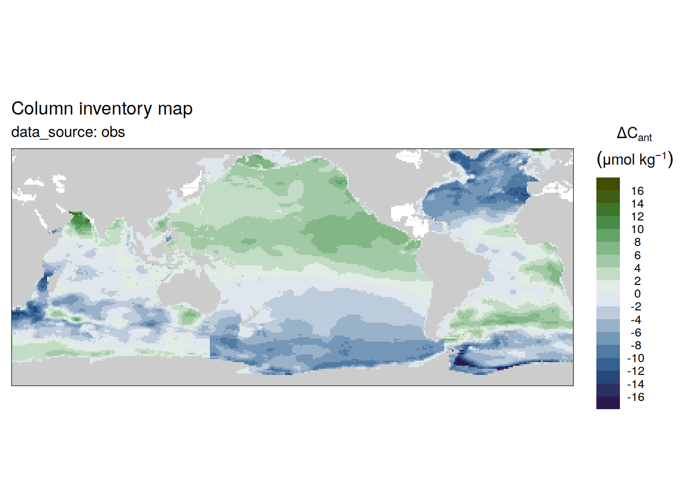
[[2]]
4.1.4 dcant pos - absolute
dcant_inv_all %>%
  filter(data_source %in% c("mod", "obs"),
         period != "1994 - 2014") %>%
  group_by(data_source) %>%
  group_split() %>%
  # head(1) %>%
  map(
    ~ p_map_cant_inv(df = .x,
                     var = "dcant_pos",
                     subtitle_text = paste("data_source:",
                                           unique(.x$data_source))) +
      facet_grid(period ~ .) +
      theme(axis.text = element_blank(),
            axis.ticks = element_blank())
  )
[[1]]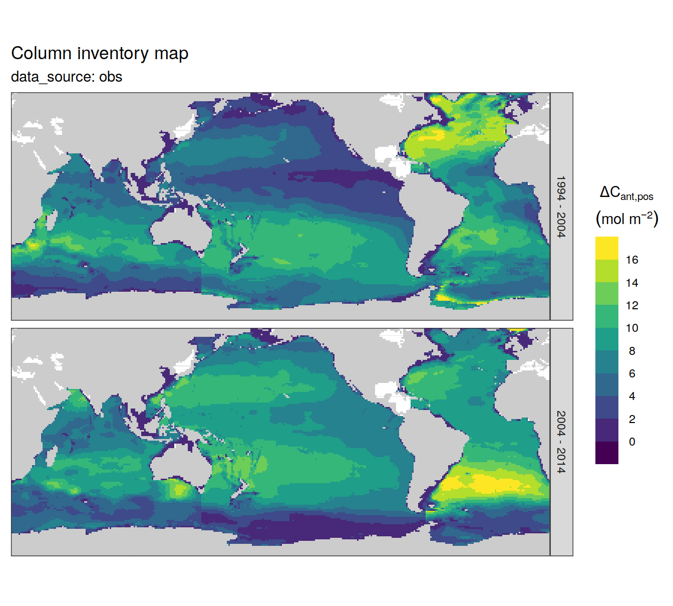
5 Zonal sections
5.1 dcant - absolut
dcant_zonal_all %>%
  filter(data_source == "obs",
         period != "1994 - 2014",
         depth <= params_global$inventory_depth_standard) %>%
  p_section_zonal_continous_depth(var = "dcant",
                                  plot_slabs = "n",
                                  title_text = NULL) +
  facet_grid(basin_AIP ~ period)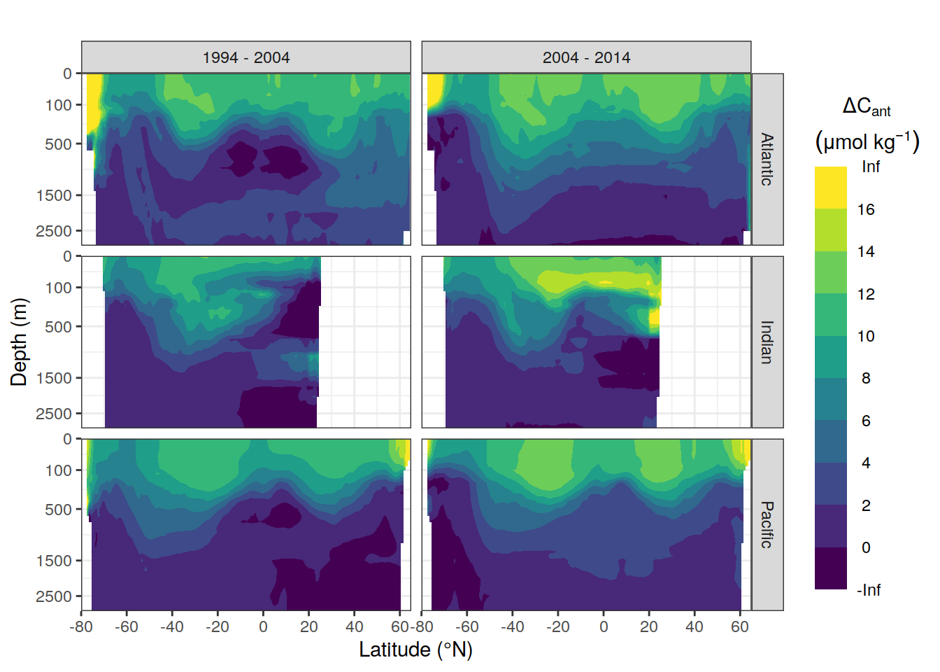
5.2 dcant - absolute delta
dcant_zonal_all %>%
  filter(data_source %in% c("mod", "obs"),
         period != "1994 - 2014") %>%
  select(data_source, lat, depth, basin_AIP, period, dcant) %>%
  pivot_wider(names_from = period,
              values_from = dcant) %>%
  mutate(delta_dcant = `2004 - 2014` - `1994 - 2004`) %>%
  group_by(data_source) %>%
  group_split() %>%
  # head(1) %>%
  map(
    ~ p_section_zonal_continous_depth(
      df = .x,
      var = "delta_dcant",
      plot_slabs = "n",
      title_text = NULL,
      col = "bias"
    ) +
      facet_grid(basin_AIP ~ .)
  )
[[1]]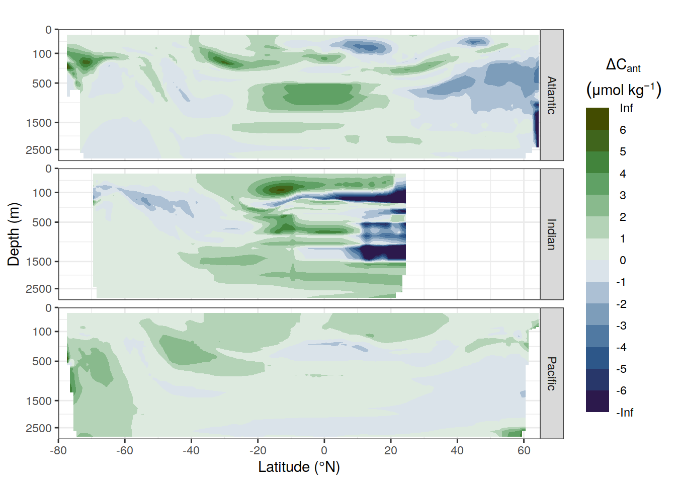
[[2]]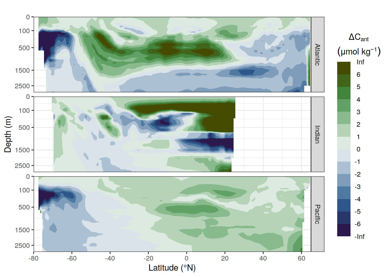
6 Concentration profiles
6.1 dcant - absolute
dcant_profile_all %>%
  arrange(depth) %>%
  filter(period != "1994 - 2014") %>%
  group_split(data_source) %>%
  # head(1) %>%
  map(
    ~ ggplot(data = .x,
             aes(dcant,
                 depth)) +
      geom_hline(yintercept = params_global$inventory_depth_standard) +
      geom_vline(xintercept = 0) +
      geom_ribbon(
        aes(
          xmin = dcant - dcant_sd,
          xmax = dcant + dcant_sd,
          fill = period
        ),
        alpha = 0.3
      ) +
      geom_path(aes(col = period)) +
      scale_y_continuous(trans = trans_reverser("sqrt"),
                         breaks = c(0, 100, 500, seq(1500, 5000, 1000))) +
      coord_cartesian(expand = 0) +
      scale_color_brewer(palette = "Set1", name = "mean \u00B1 sd", direction = -1) +
      scale_fill_brewer(palette = "Set1", name = "mean \u00B1 sd", direction = -1) +
      labs(
        title = paste("data_source", unique(.x$data_source)),
        y = "Depth (m)",
        x = dcant_umol_label
      ) +
      facet_grid(basin_AIP ~ .)
  )
[[1]]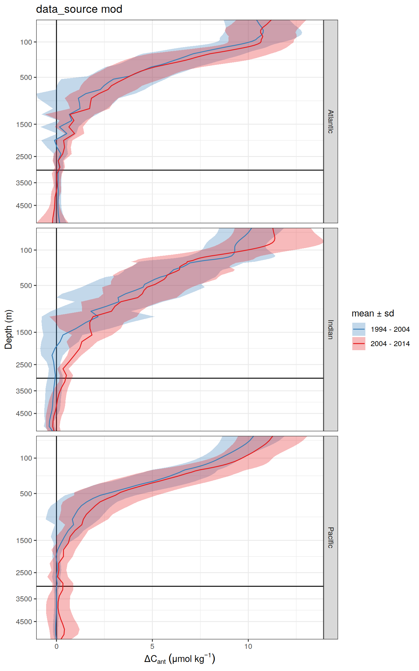
| Version | Author | Date |
|---|---|---|
| 913e42f | jens-daniel-mueller | 2022-02-01 |
| 189de95 | jens-daniel-mueller | 2022-02-01 |
| b62308d | jens-daniel-mueller | 2022-01-31 |
| 5f2aed0 | jens-daniel-mueller | 2022-01-27 |
| c6fe495 | jens-daniel-mueller | 2022-01-26 |
| 9753eb8 | jens-daniel-mueller | 2022-01-26 |
| b1d7720 | jens-daniel-mueller | 2022-01-21 |
| d6b399a | jens-daniel-mueller | 2022-01-21 |
[[2]]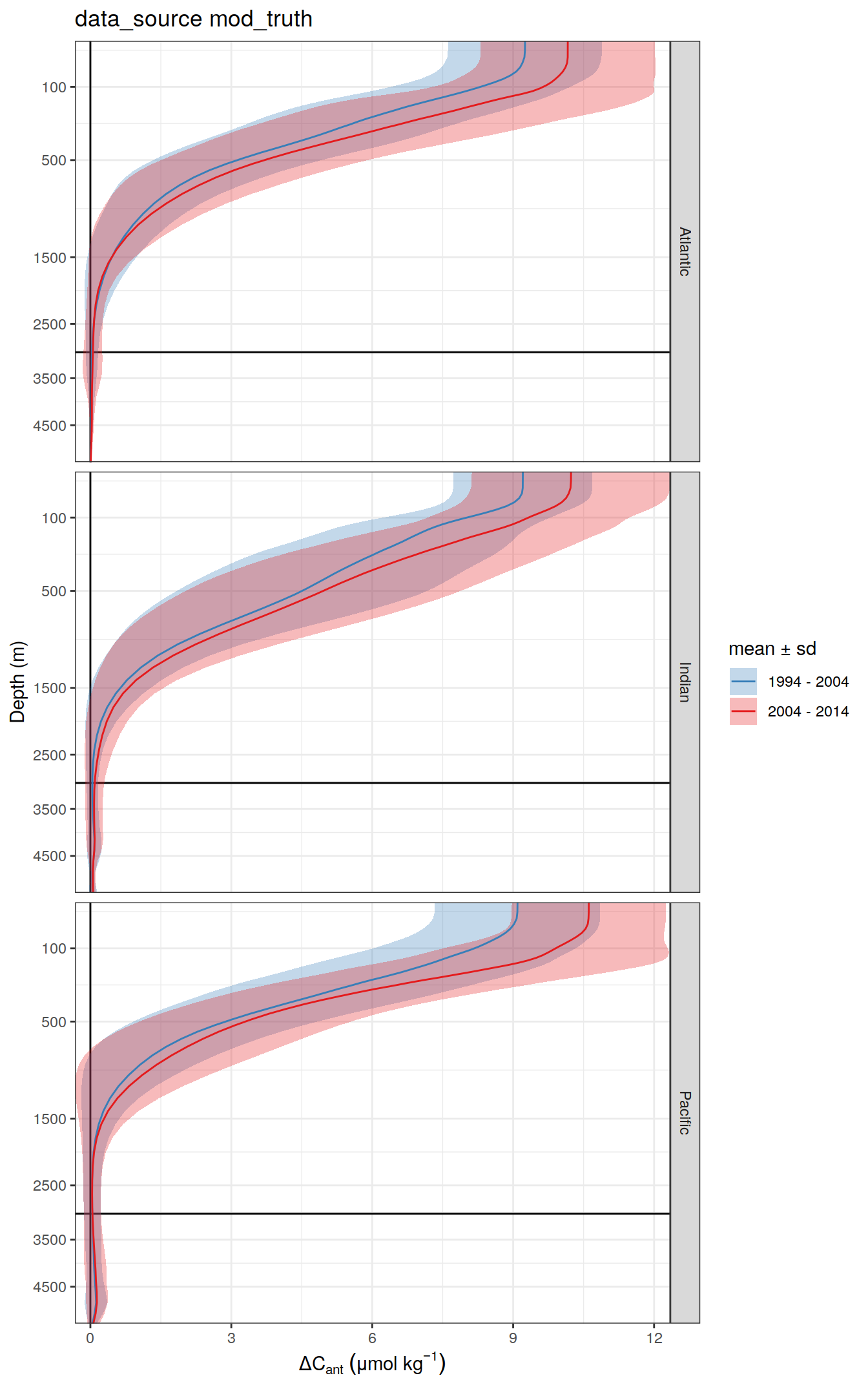
[[3]]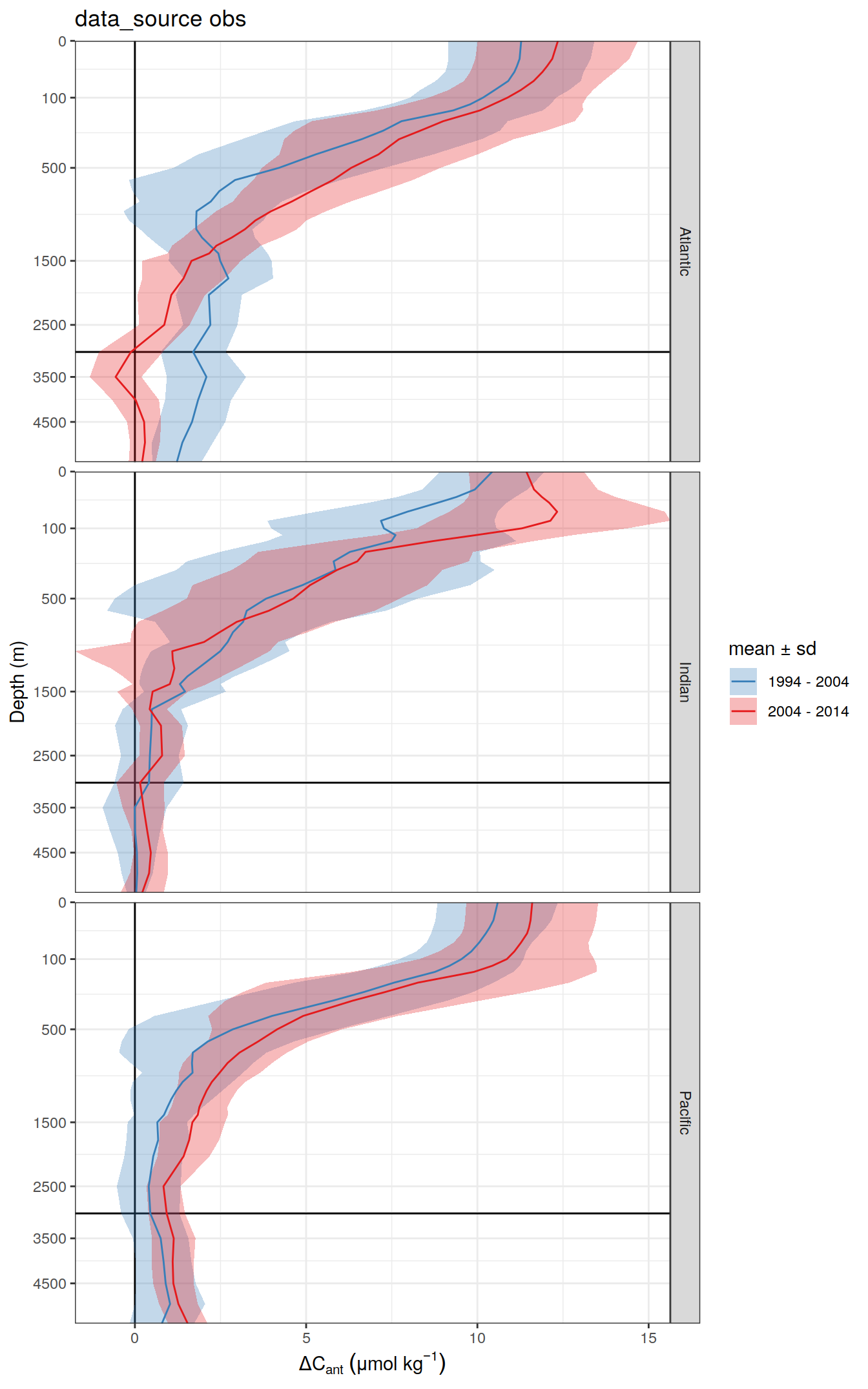
| Version | Author | Date |
|---|---|---|
| 913e42f | jens-daniel-mueller | 2022-02-01 |
| 189de95 | jens-daniel-mueller | 2022-02-01 |
| b62308d | jens-daniel-mueller | 2022-01-31 |
| 5f2aed0 | jens-daniel-mueller | 2022-01-27 |
| c6fe495 | jens-daniel-mueller | 2022-01-26 |
| 9753eb8 | jens-daniel-mueller | 2022-01-26 |
| b1d7720 | jens-daniel-mueller | 2022-01-21 |
| d6b399a | jens-daniel-mueller | 2022-01-21 |
dcant_profile_basin_MLR_all %>%
  arrange(depth) %>%
  filter(period != "1994 - 2014",
         MLR_basins == "5") %>%
    mutate(
    basin = str_replace(basin, "_", ". "),
    basin = fct_relevel(
      basin,
      "N. Pacific",
      "S. Pacific",
      "N. Atlantic",
      "S. Atlantic",
      "Indian"
    )
  ) %>%
  group_split(data_source) %>%
  # head(1) %>%
  map(
    ~ ggplot(data = .x,
             aes(dcant,
                 depth)) +
      geom_hline(yintercept = params_global$inventory_depth_standard) +
      geom_vline(xintercept = 0) +
      geom_ribbon(
        aes(
          xmin = dcant - dcant_sd,
          xmax = dcant + dcant_sd,
          fill = period
        ),
        alpha = 0.3
      ) +
      geom_path(aes(col = period)) +
      scale_y_continuous(trans = trans_reverser("sqrt"),
                         breaks = c(0, 100, 500, seq(1500, 5000, 1000))) +
      coord_cartesian(expand = 0) +
      scale_color_brewer(palette = "Set1", name = "mean \u00B1 sd", direction = -1) +
      scale_fill_brewer(palette = "Set1", name = "mean \u00B1 sd", direction = -1) +
      labs(
        title = paste("data_source", unique(.x$data_source)),
        y = "Depth (m)",
        x = dcant_umol_label
      ) +
      facet_grid(basin ~ .)
  )
[[1]]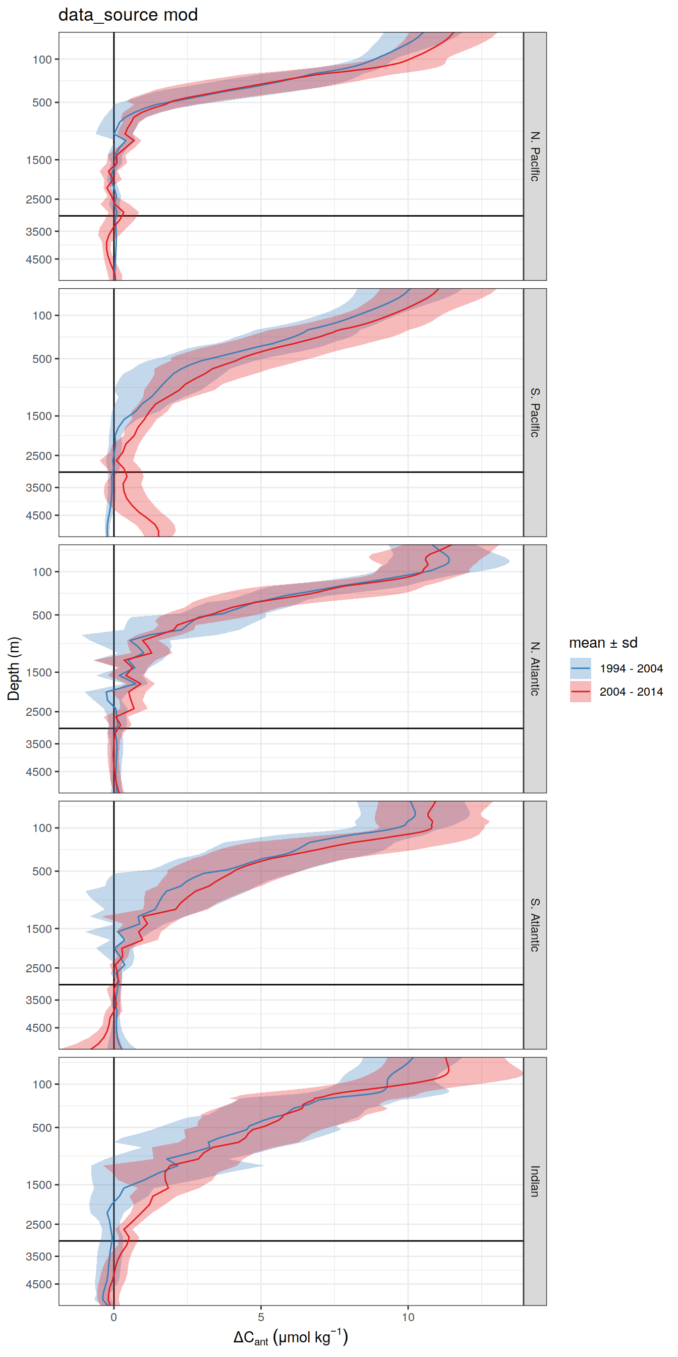
[[2]]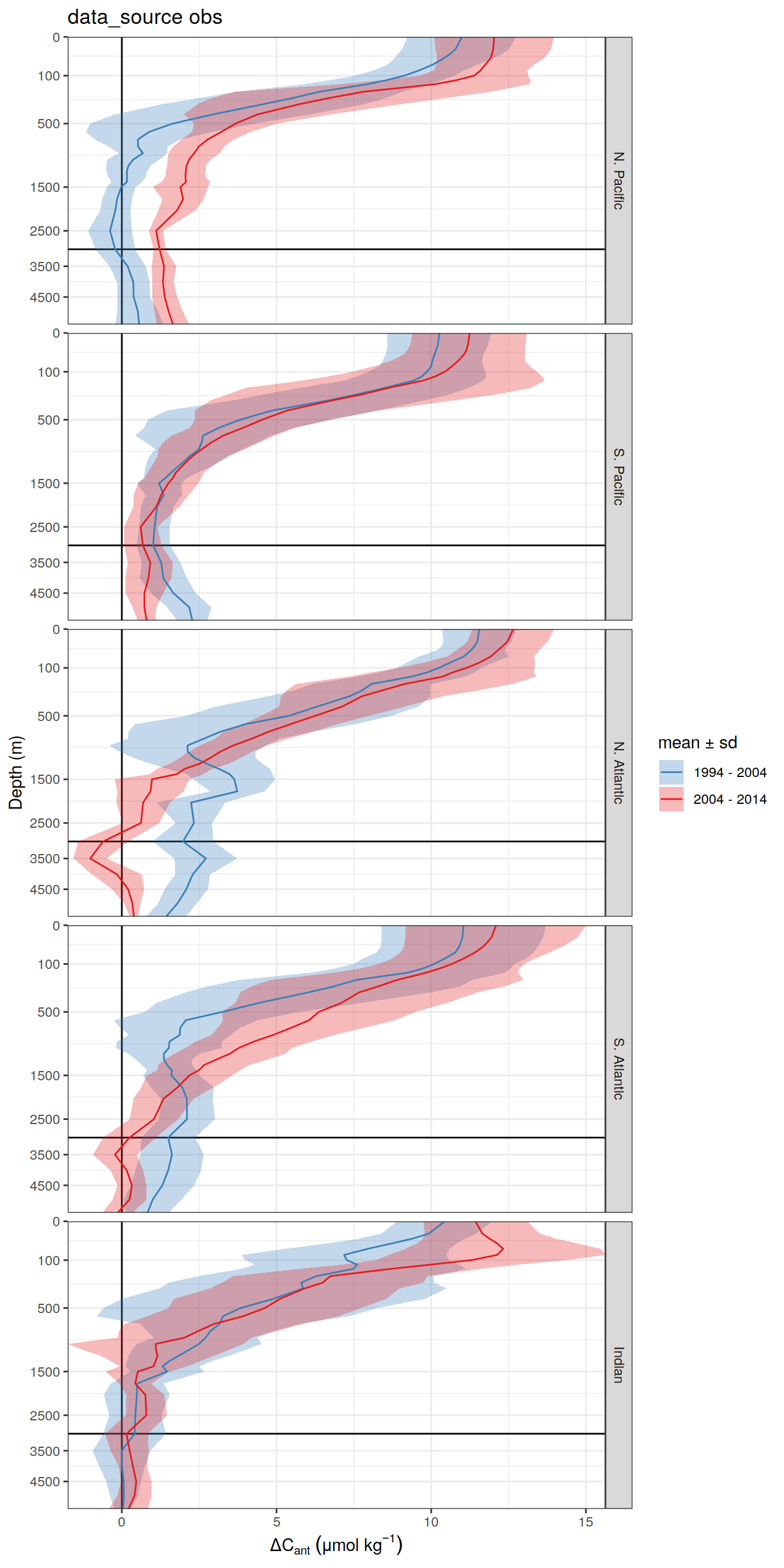
6.2 dcant - absolute delta
delta <- dcant_profile_all %>%
  arrange(depth) %>%
  filter(period != "1994 - 2014") %>%
  select(data_source, depth, basin_AIP, period, dcant) %>%
  pivot_wider(names_from = period,
              values_from = dcant) %>%
  mutate(delta_dcant = `2004 - 2014` - `1994 - 2004`) %>%
  select(-c(`2004 - 2014`, `1994 - 2004`))

delta_sd <- dcant_profile_all %>%
  arrange(depth) %>%
  filter(period != "1994 - 2014") %>%
  select(data_source, depth, basin_AIP, period, dcant_sd) %>%
  pivot_wider(names_from = period,
              values_from = dcant_sd) %>%
  mutate(delta_dcant_sd = (`2004 - 2014` + `1994 - 2004`) / 2) %>%
  select(-c(`2004 - 2014`, `1994 - 2004`))

dcant_profile_all_delta <- full_join(delta, delta_sd)
rm(delta, delta_sd)

dcant_profile_all_delta %>%
  group_split(data_source) %>%
  # head(1) %>%
  map(
    ~ ggplot(data = .x,
             aes(delta_dcant,
                 depth)) +
      geom_hline(yintercept = params_global$inventory_depth_standard) +
      geom_vline(xintercept = 0) +
      geom_ribbon(
        aes(
          xmin = delta_dcant - delta_dcant_sd,
          xmax = delta_dcant + delta_dcant_sd
        ),
        alpha = 0.3
      ) +
      geom_path() +
      scale_y_continuous(trans = trans_reverser("sqrt"),
                         breaks = c(0, 100, 500, seq(1500, 5000, 1000))) +
      coord_cartesian(expand = 0) +
      scale_color_brewer(palette = "Set1", name = "mean \u00B1 sd") +
      scale_fill_brewer(palette = "Set1", name = "mean \u00B1 sd") +
      labs(title = paste("data_source", unique(.x$data_source)),
           y = "Depth (m)",
           x = ddcant_umol_label) +
      facet_grid(basin_AIP ~ .))
[[1]]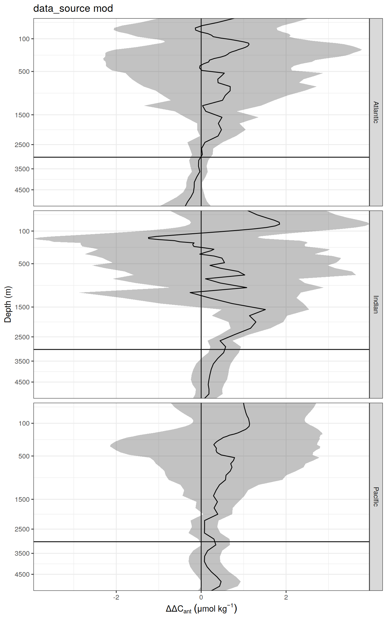
[[2]]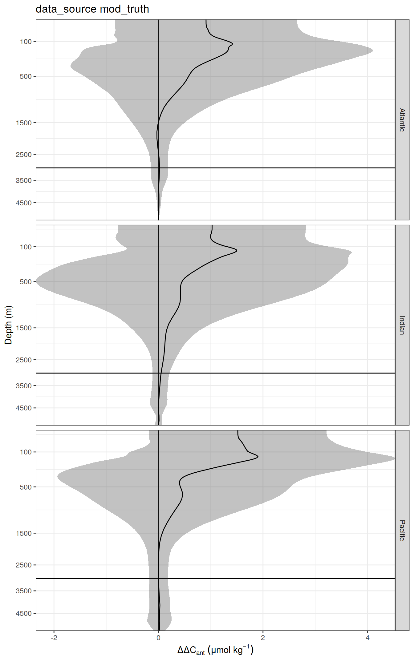
[[3]]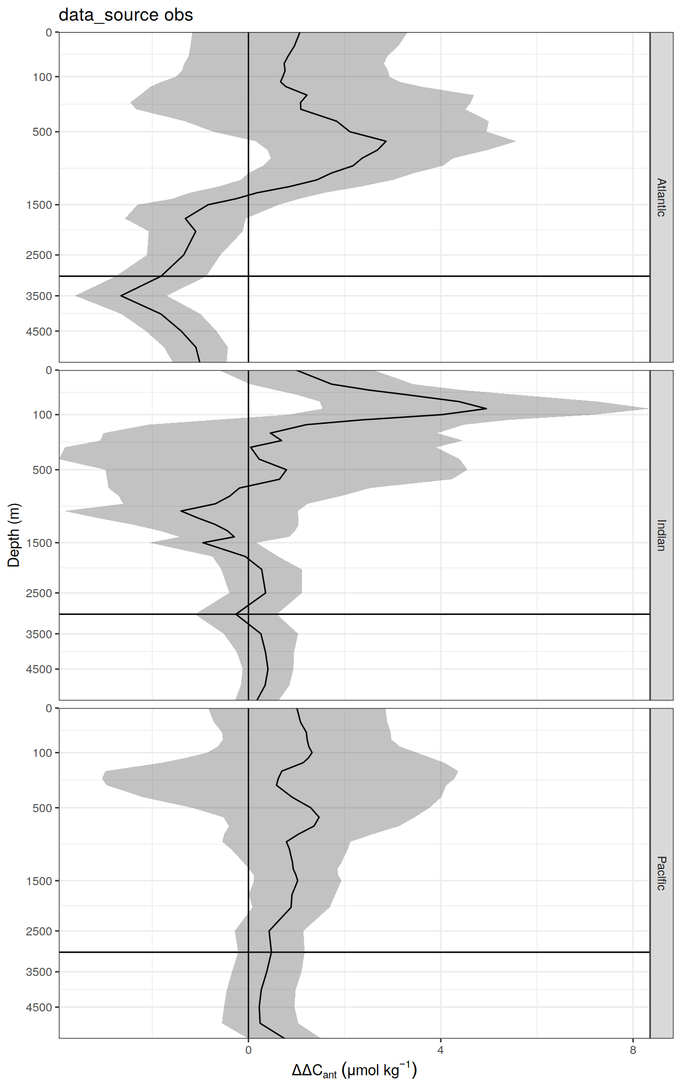
delta <- dcant_profile_basin_MLR_all %>%
  arrange(depth) %>%
  filter(period != "1994 - 2014",
         MLR_basins == "5") %>%
  select(data_source, depth, basin, period, dcant) %>%
  pivot_wider(names_from = period,
              values_from = dcant) %>%
  mutate(delta_dcant = `2004 - 2014` - `1994 - 2004`) %>%
  select(-c(`2004 - 2014`, `1994 - 2004`))

delta_sd <- dcant_profile_basin_MLR_all %>%
  arrange(depth) %>%
  filter(period != "1994 - 2014",
         MLR_basins == "5") %>%
  select(data_source, depth, basin, period, dcant_sd) %>%
  pivot_wider(names_from = period,
              values_from = dcant_sd) %>%
  mutate(delta_dcant_sd = (`2004 - 2014` + `1994 - 2004`) / 2) %>%
  select(-c(`2004 - 2014`, `1994 - 2004`))

dcant_profile_basin_MLR_all_delta <- full_join(delta, delta_sd)
rm(delta, delta_sd)


dcant_profile_basin_MLR_all_delta %>%
  mutate(
    basin = str_replace(basin, "_", ". "),
    basin = fct_relevel(
      basin,
      "N. Pacific",
      "S. Pacific",
      "N. Atlantic",
      "S. Atlantic",
      "Indian"
    )
  ) %>%
  group_split(data_source) %>%
  # head(3) %>%
  map(
    ~ ggplot(data = .x,
             aes(delta_dcant,
                 depth)) +
      geom_hline(yintercept = params_global$inventory_depth_standard) +
      geom_vline(xintercept = 0) +
      geom_ribbon(
        aes(
          xmin = delta_dcant - delta_dcant_sd,
          xmax = delta_dcant + delta_dcant_sd
        ),
        alpha = 0.3
      ) +
      geom_path() +
      scale_y_continuous(trans = trans_reverser("sqrt"),
                         breaks = c(0, 100, 500, seq(1500, 5000, 1000))) +
      coord_cartesian(expand = 0) +
      scale_color_brewer(palette = "Set1", name = "mean \u00B1 sd") +
      scale_fill_brewer(palette = "Set1", name = "mean \u00B1 sd") +
      labs(
        title = paste("data_source", unique(.x$data_source)),
        y = "Depth (m)",
        x = ddcant_umol_label
      ) +
      facet_grid(basin ~ .)
  )
[[1]]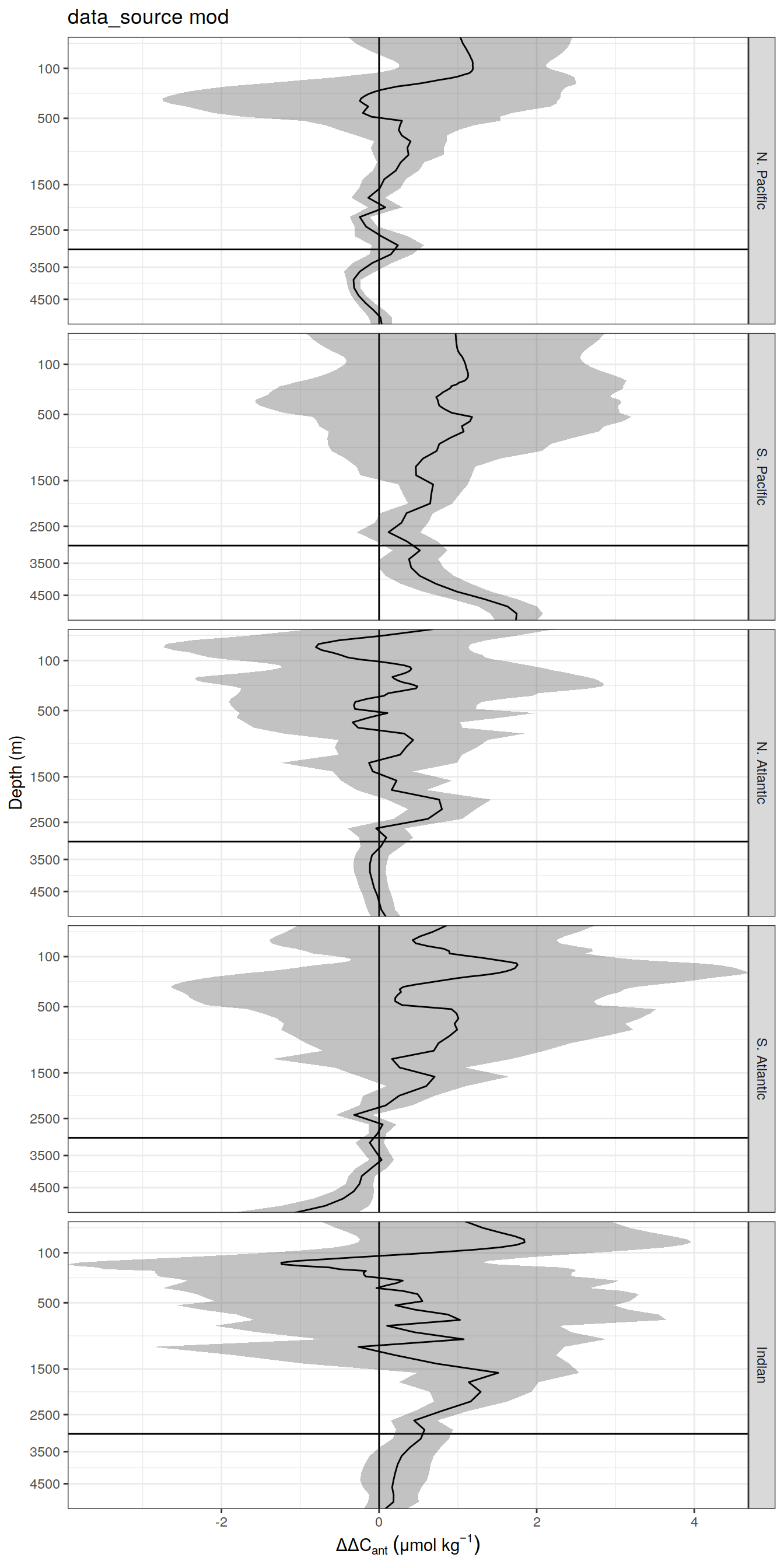
[[2]]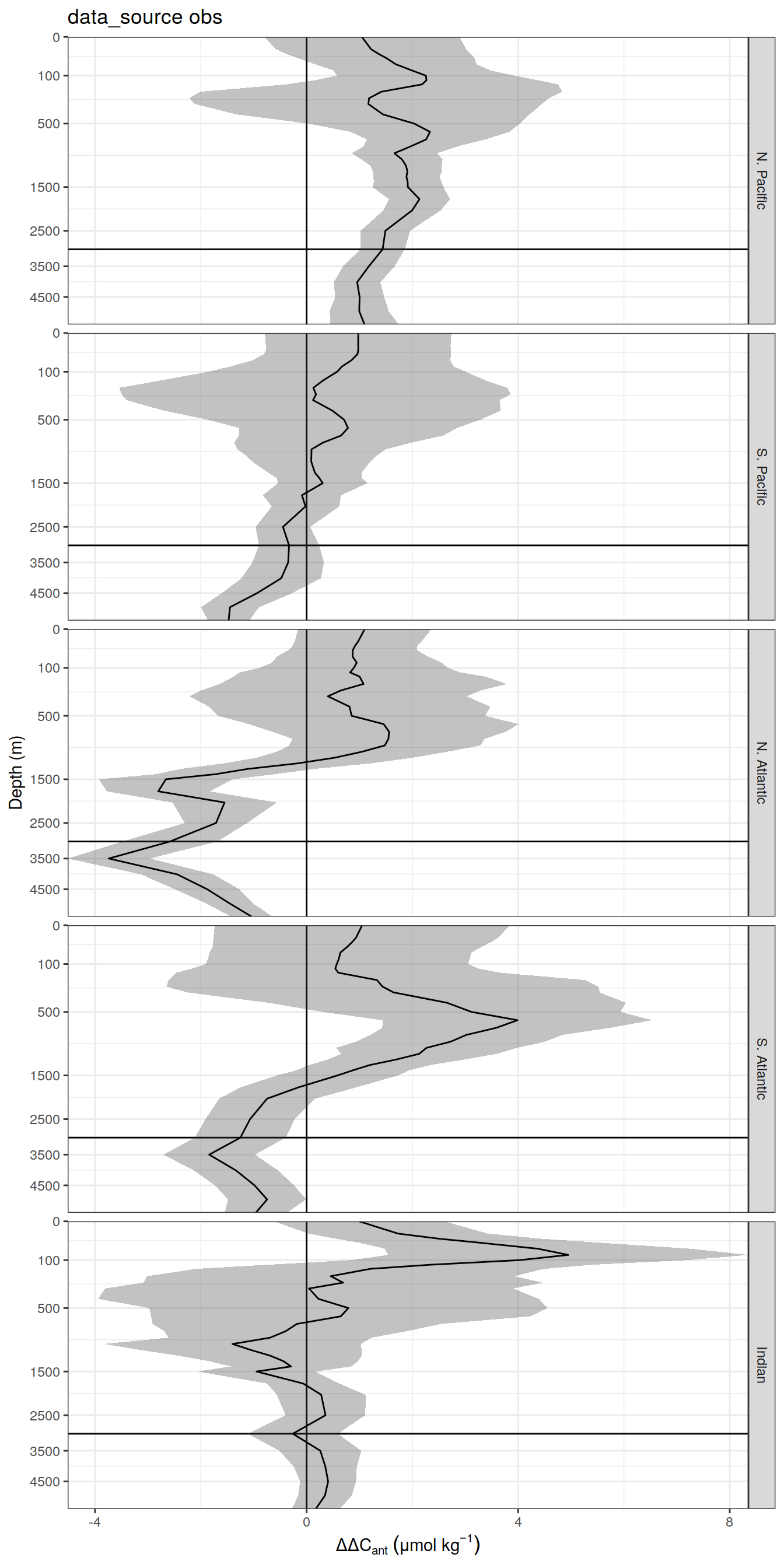
7 Budgets
7.1 Basin & hemisphere
dcant_budget_basin_MLR_all_plot <- dcant_budget_basin_MLR_all %>%
  filter(period != "1994 - 2014",
         data_source == "obs") %>%
  mutate(
    basin = str_replace(basin, "_", ". "),
        basin = fct_relevel(
      basin,
      "N. Pacific",
      "S. Pacific",
      "N. Atlantic",
      "S. Atlantic",
      "Indian"
    )
  )
g1 <- dcant_budget_basin_MLR_all_plot %>%
ggplot(aes(
y = dcant,
x = period,
alluvium = basin,
fill = basin,
stratum = basin
)) +
stat_alluvium(decreasing = FALSE) +
stat_stratum(decreasing = FALSE) +
stat_stratum(geom = "text",
decreasing = FALSE,
aes(label = paste(
round(after_stat(max-min),1)
# 100*round(after_stat(prop), 2), "%"
))) +
ggrepel::geom_label_repel(
data = dcant_budget_basin_MLR_all_plot %>% filter(period == "2004 - 2014"),
stat = "stratum",
size = 4,
nudge_x = .5,
point.padding = 3,
aes(fill = basin, label = basin),
decreasing = FALSE
)+
scale_fill_brewer(palette = "Paired", guide = "none") +
scale_y_continuous(limits = c(0, 32), expand = c(0, 0)) +
labs(y = dcant_pgc_label) +
theme(axis.text.x = element_text(angle = 45, hjust = 1),
axis.title.x = element_blank()) +
theme_classic()
newdat <- tibble(layer_data(g1))
change <-
newdat %>%
select(x, alluvium, count) %>%
pivot_wider(names_from = x,
values_from = count) %>%
mutate(dcant_change = round(100*(`2` - `1`) / `1`)) %>%
select(alluvium, dcant_change)
coord <- newdat %>%
filter(x == 2) %>%
select(x, y, alluvium)
new_layer <- full_join(
change,
coord
)
new_layer <- new_layer %>%
mutate(dcant_change = as.character(dcant_change),
dcant_change = if_else(str_detect(dcant_change, "-"),
dcant_change,
paste0("+", dcant_change)),
dcant_change = paste(dcant_change, "%"))
g1 +
geom_text(data = new_layer,
aes(
x = x - 0.3,
y = y,
label = dcant_change
),
inherit.aes = FALSE)
g2 <- dcant_budget_basin_MLR_all_plot %>%
  ggplot(aes(
    y = dcant,
    x = period,
    alluvium = basin,
    fill  = basin,
    stratum = basin,
    label = basin
  )) +
  geom_alluvium() +
  geom_stratum() +
  stat_stratum(geom = "text",
               aes(label = paste(
                 round(after_stat(count),1)
                 # 100*round(after_stat(prop), 2), "%"
                 ))) +
  ggrepel::geom_label_repel(
    data = dcant_budget_basin_MLR_all_plot %>% filter(period == "2004 - 2014"),
    stat = "stratum",
    size = 4,
    nudge_x = .5,
    point.padding = 3,
    aes(fill = basin)
  )+
  scale_fill_brewer(palette = "Paired", guide = "none") +
  scale_color_brewer(palette = "Paired", guide = "none") +
  scale_y_continuous(limits = c(0, 33), expand = c(0, 0)) +
  guides(y = "none") +
  labs(title = dcant_pgc_label) +
  theme_classic() +
  theme(axis.text.x = element_text(angle = 45, hjust = 1),
        axis.title.x = element_blank(),
        axis.title.y = element_blank(),
        plot.title = element_text(hjust = 0.5))


newdat <- tibble(layer_data(g2))

change_basin <-
  newdat %>%
  select(x, alluvium, count) %>%
  pivot_wider(names_from = x,
              values_from = count) %>%
  mutate(dcant_change = round(100*(`2` - `1`) / `1`)) %>%
  select(alluvium, dcant_change)

coord_basin <- newdat %>%
  filter(x == 2) %>%
  select(x, y, alluvium)

new_layer_basin <- full_join(
  change_basin,
  coord_basin
)

new_layer_basin <- new_layer_basin %>%
  mutate(dcant_change = as.character(dcant_change),
         dcant_change = if_else(str_detect(dcant_change, "-"),
                                dcant_change,
                                paste0("+", dcant_change)),
         dcant_change = paste(dcant_change, "%"))

new_layer_total <-
  newdat %>%
  select(x, alluvium, count) %>%
  group_by(x) %>%
  summarise(dcant_change = sum(count)) %>%
  ungroup()

new_layer_total <- new_layer_total %>%
  mutate(y = dcant_change,
         dcant_change = as.character(round(dcant_change,1)),
         dcant_change = paste("global:",dcant_change))

g2 +
  geom_text(data = new_layer_basin,
            aes(
              x = x - 0.3,
              y = y,
              label = dcant_change
            ),
            inherit.aes = FALSE) +
  geom_label(data = new_layer_total,
            aes(
              x = x,
              y = y + 1,
              label = dcant_change
            ),
            inherit.aes = FALSE)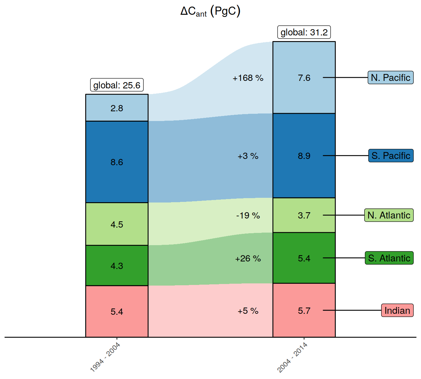
dcant_budget_basin_MLR_all_plot <- dcant_budget_basin_MLR_all_plot %>%
  filter(data_source %in% c("obs"),
         period != "1994 - 2014")

dcant_budget_basin_MLR_all_plot <- left_join(dcant_budget_basin_MLR_all_plot,
                           co2_atm %>% rename(tref1 = year,
                                              pCO21 = pCO2))

dcant_budget_basin_MLR_all_plot <- left_join(dcant_budget_basin_MLR_all_plot,
                           co2_atm %>% rename(tref2 = year,
                                              pCO22 = pCO2))

# tcant_inv <- tcant_inv %>%
#   mutate(pCO21 = 280)
#
# tcant_inv <- left_join(tcant_inv,
#                        co2_atm %>% rename(tref2 = year,
#                                           pCO22 = pCO2))
#
# dcant_budget_basin_MLR_all_plot <- bind_rows(
#   dcant_budget_basin_MLR_all_plot,
#   tcant_inv %>% mutate(period = paste(tref1, tref2, sep = " - "))
# )


dcant_budget_basin_MLR_all_plot <- dcant_budget_basin_MLR_all_plot %>%
  mutate(delta_pCO2 = pCO22 - pCO21,
         dcant_scaled = dcant / delta_pCO2) %>%
  select(-starts_with("pCO2"))


g2 <- dcant_budget_basin_MLR_all_plot %>%
  ggplot(aes(
    y = dcant_scaled,
    x = period,
    alluvium = basin,
    fill  = basin,
    stratum = basin,
    label = basin
  )) +
  geom_alluvium() +
  geom_stratum() +
  stat_stratum(geom = "text",
               aes(label = paste(
                 round(after_stat(count),2)
                 # 100*round(after_stat(prop), 2), "%"
                 ))) +
  ggrepel::geom_label_repel(
    data = dcant_budget_basin_MLR_all_plot %>% filter(period == "2004 - 2014"),
    stat = "stratum",
    size = 4,
    nudge_x = .5,
    point.padding = 3,
    aes(fill = basin)
  )+
  scale_fill_brewer(palette = "Paired", guide = "none") +
  scale_color_brewer(palette = "Paired", guide = "none") +
  # scale_y_continuous(limits = c(0, 33), expand = c(0, 0)) +
  guides(y = "none") +
  labs(title = dcant_pgc_scaled_label) +
  theme_classic() +
  theme(axis.text.x = element_text(angle = 45, hjust = 1),
        axis.title.x = element_blank(),
        axis.title.y = element_blank(),
        plot.title = element_text(hjust = 0.5))


newdat <- tibble(layer_data(g2))

change_basin <-
  newdat %>%
  select(x, alluvium, count) %>%
  pivot_wider(names_from = x,
              values_from = count) %>%
  mutate(dcant_change = round(100*(`2` - `1`) / `1`)) %>%
  select(alluvium, dcant_change)

coord_basin <- newdat %>%
  filter(x == 2) %>%
  select(x, y, alluvium)

new_layer_basin <- full_join(
  change_basin,
  coord_basin
)

new_layer_basin <- new_layer_basin %>%
  mutate(dcant_change = as.character(dcant_change),
         dcant_change = if_else(str_detect(dcant_change, "-"),
                                dcant_change,
                                paste0("+", dcant_change)),
         dcant_change = paste(dcant_change, "%"))

new_layer_total <-
  newdat %>%
  select(x, alluvium, count) %>%
  group_by(x) %>%
  summarise(dcant_change = sum(count)) %>%
  ungroup()

new_layer_total <- new_layer_total %>%
  mutate(y = dcant_change,
         dcant_change = as.character(round(dcant_change,2)),
         dcant_change = paste("global:",dcant_change))

g2 +
  geom_text(data = new_layer_basin,
            aes(
              x = x - 0.3,
              y = y,
              label = dcant_change
            ),
            inherit.aes = FALSE) +
  geom_label(data = new_layer_total,
            aes(
              x = x,
              y = y + 0.05,
              label = dcant_change
            ),
            inherit.aes = FALSE)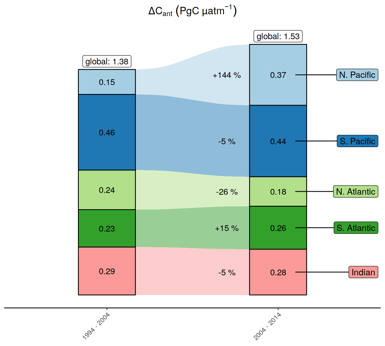
7.2 Depth layer
7.2.1 Basin AIP
dcant_budget_basin_AIP_layer_all %>%
  filter(estimate == "dcant",
         period != "1994 - 2014",
         inv_depth <= 3000,
         data_source == "obs") %>%
  rename(dcant = value) %>%
  ggplot(aes(inv_depth-250, dcant, col=period)) +
  geom_hline(yintercept = 0) +
  geom_step(direction = "vh") +
  coord_flip() +
  scale_x_reverse(breaks = seq(0, 3000, 500)) +
  scale_color_brewer(palette = "Set1", direction = -1) +
  facet_grid(basin_AIP ~ .) +
  labs(y = dcant_layer_budget_label,
       x = "Depth (m)")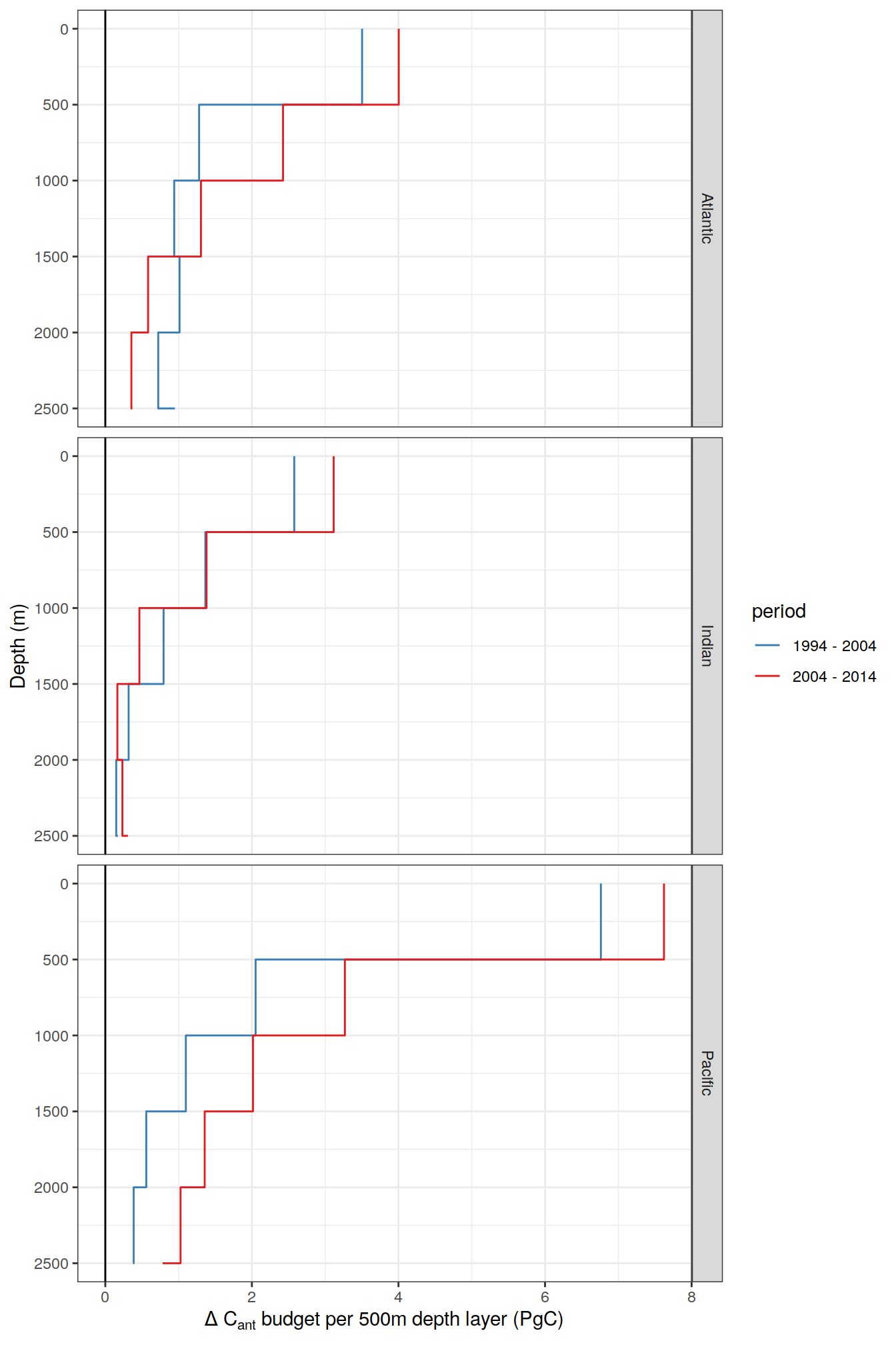
7.2.2 5 basins
dcant_budget_change <- dcant_budget_basin_MLR_layer_all %>%
  filter(estimate == "dcant",
         period != "1994 - 2014",
         inv_depth <= 3000,
         data_source == "obs") %>%
  rename(dcant = value) %>%
  select(-c(tref2, Version_ID)) %>%
  pivot_wider(names_from = period,
              values_from = dcant) %>%
  mutate(sign = if_else(`2004 - 2014` - `1994 - 2004` > 0,
                        "increase",
                        "decrease")) %>%
  mutate(
    basin = str_replace(basin, "_", ". "),
    basin = fct_relevel(
      basin,
      "N. Pacific",
      "S. Pacific",
      "N. Atlantic",
      "S. Atlantic",
      "Indian"
    )
  )

dcant_budget_layer <- dcant_budget_basin_MLR_layer_all %>%
  filter(estimate == "dcant",
         period != "1994 - 2014",
         inv_depth <= 3400,
         data_source == "obs") %>%
  rename(dcant = value) %>%
  mutate(
    basin = str_replace(basin, "_", ". "),
    basin = fct_relevel(
      basin,
      "N. Pacific",
      "S. Pacific",
      "N. Atlantic",
      "S. Atlantic",
      "Indian"
    )
  ) %>%
  group_by(basin, period, data_source) %>%
  mutate(dcant = if_else(is.na(lead(dcant)), 888, dcant),
         dcant = na_if(dcant, 888)) %>%
  fill(dcant) %>%
  ungroup()

dcant_budget_layer %>%
  ggplot() +
  geom_hline(yintercept = 0) +
  geom_rect(
    data = dcant_budget_change,
    aes(
      xmin = inv_depth - 250,
      xmax = inv_depth + 250,
      ymin = `1994 - 2004`,
      ymax = `2004 - 2014`,
      fill = sign
    ),
    alpha = 0.3
  ) +
  geom_step(aes(inv_depth - 250, dcant, col = period), direction = "vh",
            size = 1) +
  coord_flip() +
  scale_x_reverse(breaks = seq(0, 3000, 500)) +
  scale_color_brewer(palette = "Set1", direction = -1, name = "Decade") +
  scale_fill_brewer(palette = "Set1", direction = -1, name = "Decadal change") +
  facet_grid(basin ~ .) +
  labs(y = dcant_layer_budget_label,
       x = "Depth (m)",
       title = "Layer inventory change")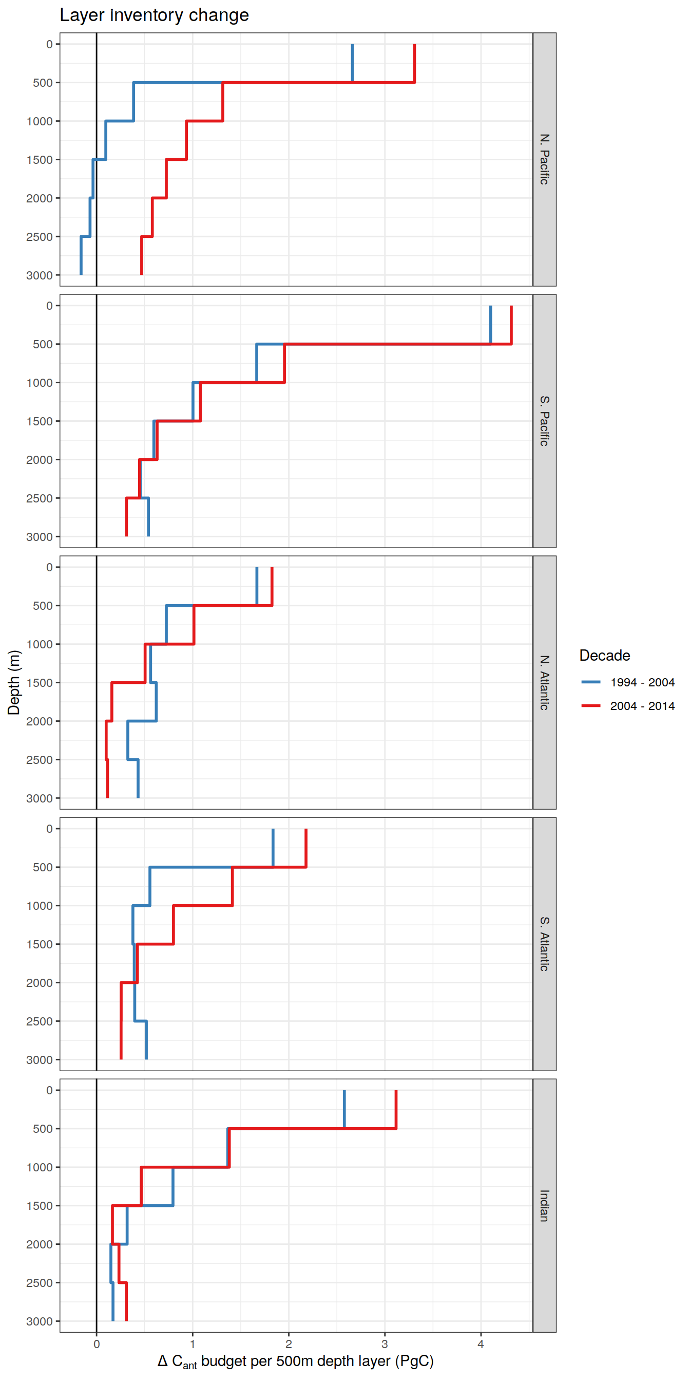
dcant_budget_change <- dcant_budget_basin_MLR_layer_all %>%
  filter(estimate == "dcant",
         period != "1994 - 2014",
         inv_depth <= 3000,
         data_source == "obs") %>%
  rename(dcant = value) %>%
  arrange(inv_depth) %>%
  group_by(data_source, basin, period) %>%
  mutate(dcant_cum = cumsum(dcant)) %>%
  ungroup() %>%
  select(-c(tref2, Version_ID, dcant)) %>%
  pivot_wider(names_from = period,
              values_from = dcant_cum) %>%
  mutate(sign = if_else(`2004 - 2014` - `1994 - 2004` > 0,
                        "increase",
                        "decrease")) %>%
  mutate(
    basin = str_replace(basin, "_", ". "),
    basin = fct_relevel(
      basin,
      "N. Pacific",
      "S. Pacific",
      "N. Atlantic",
      "S. Atlantic",
      "Indian"
    )
  )

dcant_budget_layer <- dcant_budget_basin_MLR_layer_all %>%
  filter(estimate == "dcant",
         period != "1994 - 2014",
         inv_depth <= 3400,
         data_source == "obs") %>%
  rename(dcant = value) %>%
  arrange(inv_depth) %>%
  group_by(data_source, basin, period) %>%
  mutate(dcant_cum = cumsum(dcant)) %>%
  ungroup() %>%
  mutate(
    basin = str_replace(basin, "_", ". "),
    basin = fct_relevel(
      basin,
      "N. Pacific",
      "S. Pacific",
      "N. Atlantic",
      "S. Atlantic",
      "Indian"
    )
  ) %>%
  group_by(basin, period, data_source) %>%
  mutate(dcant_cum = if_else(is.na(lead(dcant_cum)), 888, dcant_cum),
         dcant_cum = na_if(dcant_cum, 888)) %>%
  fill(dcant_cum) %>%
  ungroup()


dcant_budget_layer %>%
  ggplot() +
  geom_hline(yintercept = 0) +
  geom_rect(
    data = dcant_budget_change,
    aes(
      xmin = inv_depth - 250,
      xmax = inv_depth + 250,
      ymin = `1994 - 2004`,
      ymax = `2004 - 2014`,
      fill = sign
    ),
    alpha = 0.3
  ) +
  geom_step(aes(inv_depth - 250, dcant_cum, col = period), direction = "vh",
            size = 1) +
  coord_flip() +
  scale_x_reverse(breaks = seq(0, 3000, 500)) +
  scale_color_brewer(palette = "Set1", direction = -1, name = "Decade") +
  scale_fill_brewer(palette = "Set1", direction = -1, name = "Decadal change") +
  facet_grid(basin ~ .) +
  labs(y = dcant_layer_budget_label,
       x = "Depth (m)",
       title = "Cumulative layer inventory change")
8 Time series
dcant_budget_global_ts <- dcant_budget_global_all %>%
  filter(data_source == "obs",
         period != "1994 - 2014") %>%
  select(year = tref2, dcant_mean = dcant) %>%
  mutate(dcant_sd = 3)

tcant_S04 <- bind_cols(year = 1994, dcant_mean = 118, dcant_sd = 19)

tcant_ts <- full_join(dcant_budget_global_ts, tcant_S04)

tcant_ts <- left_join(tcant_ts, co2_atm)

co2_atm_pi <- bind_cols(pCO2 = 280, dcant_mean = 0, year = 1750, dcant_sd = 0)

tcant_ts <- full_join(tcant_ts, co2_atm_pi)

tcant_ts <- tcant_ts %>%
  arrange(year) %>%
  mutate(tcant = cumsum(dcant_mean),
         tcant_sd = cumsum(dcant_sd))

tcant_ts %>%
  ggplot(aes(pCO2, tcant, ymin = tcant - tcant_sd, ymax = tcant + tcant_sd)) +
  geom_ribbon(fill = "grey80") +
  geom_point() +
  geom_line() +
  scale_x_continuous(breaks = seq(280, 400, 30),
                     sec.axis = dup_axis(labels =  c(1750, 1940, 1980, 2000, 2015),
                                         name = "Year")) +
  geom_text(aes(label = year), nudge_x = -5, nudge_y = 5) +
  labs(x = expression(Atmospheric~pCO[2]~(µatm)),
       y = expression(Total~oceanic~C[ant]~(PgC)))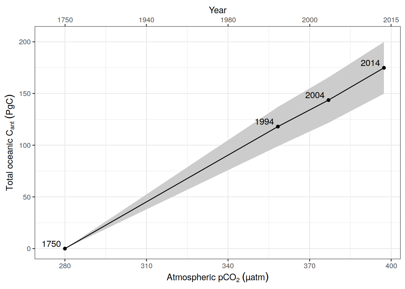
| Version | Author | Date |
|---|---|---|
| ec7fe7e | jens-daniel-mueller | 2022-01-31 |
# ggsave(path = "output/publication",
#        filename = "Fig_global_dcant_budget_vs_atm_pCO2.png",
#        height = 4,
#        width = 7)
sessionInfo()R version 4.1.2 (2021-11-01)
Platform: x86_64-pc-linux-gnu (64-bit)
Running under: openSUSE Leap 15.3
Matrix products: default
BLAS: /usr/local/R-4.1.2/lib64/R/lib/libRblas.so
LAPACK: /usr/local/R-4.1.2/lib64/R/lib/libRlapack.so
locale:
[1] LC_CTYPE=en_US.UTF-8 LC_NUMERIC=C
[3] LC_TIME=en_US.UTF-8 LC_COLLATE=en_US.UTF-8
[5] LC_MONETARY=en_US.UTF-8 LC_MESSAGES=en_US.UTF-8
[7] LC_PAPER=en_US.UTF-8 LC_NAME=C
[9] LC_ADDRESS=C LC_TELEPHONE=C
[11] LC_MEASUREMENT=en_US.UTF-8 LC_IDENTIFICATION=C
attached base packages:
[1] stats graphics grDevices utils datasets methods base
other attached packages:
[1] ggalluvial_0.12.3 ggforce_0.3.3 metR_0.11.0 scico_1.3.0
[5] patchwork_1.1.1 collapse_1.7.0 forcats_0.5.1 stringr_1.4.0
[9] dplyr_1.0.7 purrr_0.3.4 readr_2.1.1 tidyr_1.1.4
[13] tibble_3.1.6 ggplot2_3.3.5 tidyverse_1.3.1 workflowr_1.7.0
loaded via a namespace (and not attached):
[1] fs_1.5.2 lubridate_1.8.0 bit64_4.0.5 RColorBrewer_1.1-2
[5] httr_1.4.2 rprojroot_2.0.2 tools_4.1.2 backports_1.4.1
[9] bslib_0.3.1 utf8_1.2.2 R6_2.5.1 DBI_1.1.2
[13] colorspace_2.0-2 withr_2.4.3 tidyselect_1.1.1 processx_3.5.2
[17] bit_4.0.4 compiler_4.1.2 git2r_0.29.0 cli_3.1.1
[21] rvest_1.0.2 xml2_1.3.3 isoband_0.2.5 labeling_0.4.2
[25] sass_0.4.0 scales_1.1.1 checkmate_2.0.0 callr_3.7.0
[29] digest_0.6.29 rmarkdown_2.11 pkgconfig_2.0.3 htmltools_0.5.2
[33] highr_0.9 dbplyr_2.1.1 fastmap_1.1.0 rlang_0.4.12
[37] readxl_1.3.1 rstudioapi_0.13 jquerylib_0.1.4 generics_0.1.1
[41] farver_2.1.0 jsonlite_1.7.3 vroom_1.5.7 magrittr_2.0.1
[45] Rcpp_1.0.8 munsell_0.5.0 fansi_1.0.2 lifecycle_1.0.1
[49] stringi_1.7.6 whisker_0.4 yaml_2.2.1 MASS_7.3-55
[53] grid_4.1.2 ggrepel_0.9.1 parallel_4.1.2 promises_1.2.0.1
[57] crayon_1.4.2 haven_2.4.3 hms_1.1.1 knitr_1.37
[61] ps_1.6.0 pillar_1.6.4 reprex_2.0.1 glue_1.6.0
[65] evaluate_0.14 getPass_0.2-2 data.table_1.14.2 modelr_0.1.8
[69] vctrs_0.3.8 tzdb_0.2.0 tweenr_1.0.2 httpuv_1.6.5
[73] cellranger_1.1.0 gtable_0.3.0 polyclip_1.10-0 assertthat_0.2.1
[77] xfun_0.29 broom_0.7.11 later_1.3.0 viridisLite_0.4.0
[81] ellipsis_0.3.2