GLODAPv2_2020
Jens Daniel Müller
02 December, 2020
Last updated: 2020-12-02
Checks: 7 0
Knit directory: emlr_obs_v_XXX/
This reproducible R Markdown analysis was created with workflowr (version 1.6.2). The Checks tab describes the reproducibility checks that were applied when the results were created. The Past versions tab lists the development history.
Great! Since the R Markdown file has been committed to the Git repository, you know the exact version of the code that produced these results.
Great job! The global environment was empty. Objects defined in the global environment can affect the analysis in your R Markdown file in unknown ways. For reproduciblity it’s best to always run the code in an empty environment.
The command set.seed(20200707) was run prior to running the code in the R Markdown file. Setting a seed ensures that any results that rely on randomness, e.g. subsampling or permutations, are reproducible.
Great job! Recording the operating system, R version, and package versions is critical for reproducibility.
Nice! There were no cached chunks for this analysis, so you can be confident that you successfully produced the results during this run.
Great job! Using relative paths to the files within your workflowr project makes it easier to run your code on other machines.
Great! You are using Git for version control. Tracking code development and connecting the code version to the results is critical for reproducibility.
The results in this page were generated with repository version 9ff071b. See the Past versions tab to see a history of the changes made to the R Markdown and HTML files.
Note that you need to be careful to ensure that all relevant files for the analysis have been committed to Git prior to generating the results (you can use wflow_publish or wflow_git_commit). workflowr only checks the R Markdown file, but you know if there are other scripts or data files that it depends on. Below is the status of the Git repository when the results were generated:
Ignored files:
    Ignored:    .Rhistory
    Ignored:    .Rproj.user/

Unstaged changes:
    Modified:   README.md
    Modified:   code/Workflowr_project_managment.R
Note that any generated files, e.g. HTML, png, CSS, etc., are not included in this status report because it is ok for generated content to have uncommitted changes.
These are the previous versions of the repository in which changes were made to the R Markdown (analysis/eMLR_GLODAPv2_2020_subsetting.Rmd) and HTML (docs/eMLR_GLODAPv2_2020_subsetting.html) files. If you’ve configured a remote Git repository (see ?wflow_git_remote), click on the hyperlinks in the table below to view the files as they were in that past version.
| File | Version | Author | Date | Message |
|---|---|---|---|---|
| Rmd | 9ff071b | jens-daniel-mueller | 2020-12-02 | minor improvement of tref adejustment, formatting |
| html | 7c25f7a | jens-daniel-mueller | 2020-12-02 | Build site. |
| Rmd | 5ffd065 | jens-daniel-mueller | 2020-12-02 | rebuild with nice era labels |
| html | ec8dc38 | jens-daniel-mueller | 2020-12-02 | Build site. |
| html | c987de1 | jens-daniel-mueller | 2020-12-02 | Build site. |
| html | d5c5378 | jens-daniel-mueller | 2020-12-02 | Build site. |
| Rmd | 3cc6d3c | jens-daniel-mueller | 2020-12-02 | code cleaning and commenting |
| html | 083b3b0 | jens-daniel-mueller | 2020-12-02 | Build site. |
| Rmd | f4520b2 | jens-daniel-mueller | 2020-12-02 | code cleaning and commenting |
| html | 632c84f | jens-daniel-mueller | 2020-12-02 | Build site. |
| Rmd | 8f3d29d | jens-daniel-mueller | 2020-12-02 | code cleaning and commenting |
| html | 22d0127 | jens-daniel-mueller | 2020-12-01 | Build site. |
| html | 0ff728b | jens-daniel-mueller | 2020-12-01 | Build site. |
| Rmd | 6287a18 | jens-daniel-mueller | 2020-12-01 | auto eras naming |
| html | b02b7a4 | jens-daniel-mueller | 2020-12-01 | Build site. |
| Rmd | 60bea48 | jens-daniel-mueller | 2020-12-01 | auto eras naming |
| html | cf19652 | jens-daniel-mueller | 2020-11-30 | Build site. |
| html | 196be51 | jens-daniel-mueller | 2020-11-30 | Build site. |
| Rmd | 7a4b015 | jens-daniel-mueller | 2020-11-30 | first rebuild on ETH server |
1 Read files
Main data source for this project is the preprocessed version of the GLODAPv2.2020_Merged_Master_File.csv downloaded from glodap.info in June 2020.
GLODAP <-
  read_csv(paste(path_preprocessing,
                 "GLODAPv2.2020_preprocessed.csv",
                 sep = ""))
2 Data preparation
2.1 Reference eras
Samples were assigned to following eras:
# create clear labels for era
labels <- bind_cols(
  start = params_local$era_breaks+1,
  end = lead(params_local$era_breaks))

labels <- labels %>%
  filter(!is.na(end)) %>%
  mutate(end = if_else(end == Inf, max(GLODAP$year), end),
         label = paste(start, end, sep = "-")) %>%
  select(label) %>%
  pull()

# cut observation years into era applying the labels
GLODAP <- GLODAP %>%
  filter(year > params_local$era_breaks[1]) %>%
  mutate(era = cut(year,
                   params_local$era_breaks,
                   labels = labels))

levels(GLODAP$era)
[1] "1982-1999" "2000-2012" "2013-2019"rm(labels)2.2 Spatial boundaries
2.2.1 Depth
Observations collected shallower than:
- minimum sampling depth: 150m
were excluded from the analysis to avoid seasonal bias.
GLODAP <- GLODAP %>%
  filter(depth >= params_local$depth_min)
2.2.2 Bottomdepth
Observations collected in an area with a:
- minimum bottom depth: 0m
were excluded from the analysis to avoid coastal impacts. Please note that minimum bottom depth criterion of 0m means that no filtering was applied here.
GLODAP <- GLODAP %>%
  filter(bottomdepth >= params_local$bottomdepth_min)
2.3 Flags and missing data
Only rows (samples) for which all relevant parameters are available were selected, ie NA’s were removed.
According to Olsen et al (2020), flags within the merged master file identify:
f:
- 2: Acceptable
- 0: Interpolated (nutrients/oxygen) or calculated (CO[2] params_local) value
- 9: Data not used (so, only NA data should have this flag)
qc:
- 1: Adjusted or unadjusted data
- 0: Data appear of good quality but have not been subjected to full secondary QC
- data with poor or uncertain quality are excluded.
Following flagging criteria were taken into account:
- flag_f: 2, 0
- flag_qc: 1
Summary statistics were calculated during cleaning process.
2.3.1 tco2
2.3.1.1 NA
Rows with missing tco2 observations were already removed in the preprocessing.
GLODAP_stats <- GLODAP %>%
  summarise(tco2_values = n())

GLODAP_obs_grid <- GLODAP %>%
  count(lat, lon, era) %>%
  mutate(cleaning_level = "tco2_values")
GLODAP_obs <- GLODAP %>%
group_by(lat, lon) %>%
summarise(n = n()) %>%
ungroup()
map +
geom_raster(data = basinmask, aes(lon, lat, fill = basin)) +
geom_raster(data = GLODAP_obs, aes(lon, lat)) +
scale_fill_brewer(palette = "Dark2") +
theme(legend.position = "top",
legend.title = element_blank())
rm(GLODAP_obs)2.3.1.2 f flag
GLODAP_obs_grid_temp <- GLODAP %>%
  count(lat, lon, era, tco2f)

map +
  geom_raster(data = GLODAP_obs_grid_temp, aes(lon, lat, fill = n)) +
  scale_fill_viridis_c(option = "magma",
                       direction = -1,
                       trans = "log10") +
  facet_grid(era ~ tco2f) +
  theme(legend.position = "top")
rm(GLODAP_obs_grid_temp)

GLODAP <- GLODAP %>%
  filter(tco2f %in% params_local$flag_f)
2.3.1.3 qc flag
GLODAP_obs_grid_temp <- GLODAP %>%
  count(lat, lon, era, tco2qc)

map +
  geom_raster(data = GLODAP_obs_grid_temp, aes(lon, lat, fill = n)) +
  scale_fill_viridis_c(option = "magma",
                       direction = -1,
                       trans = "log10") +
  facet_grid(era ~ tco2qc) +
  theme(legend.position = "top")
##

GLODAP <- GLODAP %>%
  filter(tco2qc %in% params_local$flag_qc)

GLODAP_stats_temp <- GLODAP %>%
  summarise(tco2_flag = n())

GLODAP_stats <- cbind(GLODAP_stats, GLODAP_stats_temp)
rm(GLODAP_stats_temp)

##

GLODAP_obs_grid_temp <- GLODAP %>%
  count(lat, lon, era) %>%
  mutate(cleaning_level = "tco2_flag")

GLODAP_obs_grid <-
  bind_rows(GLODAP_obs_grid, GLODAP_obs_grid_temp)

rm(GLODAP_obs_grid_temp)
2.3.2 talk
2.3.2.1 NA
GLODAP <- GLODAP %>%
  mutate(talkna = if_else(is.na(talk), "NA", "Value"))

GLODAP_obs_grid_temp <- GLODAP %>%
  count(lat, lon, era, talkna)

map +
  geom_raster(data = GLODAP_obs_grid_temp, aes(lon, lat, fill = n)) +
  scale_fill_viridis_c(option = "magma",
                       direction = -1,
                       trans = "log10") +
  facet_grid(era ~ talkna) +
  theme(legend.position = "top")
GLODAP <- GLODAP %>%
  select(-talkna) %>%
  filter(!is.na(talk))

##

GLODAP_stats_temp <- GLODAP %>%
  summarise(talk_values = n())

GLODAP_stats <- cbind(GLODAP_stats, GLODAP_stats_temp)
rm(GLODAP_stats_temp)

##

GLODAP_obs_grid_temp <- GLODAP %>%
  count(lat, lon, era) %>%
  mutate(cleaning_level = "talk_values")

GLODAP_obs_grid <-
  bind_rows(GLODAP_obs_grid, GLODAP_obs_grid_temp)

rm(GLODAP_obs_grid_temp)
2.3.2.2 f flag
GLODAP_obs_grid_temp <- GLODAP %>%
  count(lat, lon, era, talkf)

map +
  geom_raster(data = GLODAP_obs_grid_temp, aes(lon, lat, fill = n)) +
  scale_fill_viridis_c(option = "magma",
                       direction = -1,
                       trans = "log10") +
  facet_grid(era ~ talkf) +
  theme(legend.position = "top",
        legend.title = element_blank())
# ###

GLODAP <- GLODAP %>%
  filter(talkf %in% params_local$flag_f)
2.3.2.3 qc flag
GLODAP_obs_grid_temp <- GLODAP %>%
  count(lat, lon, era, talkqc)

map +
  geom_raster(data = GLODAP_obs_grid_temp, aes(lon, lat, fill = n)) +
  scale_fill_viridis_c(option = "magma",
                       direction = -1,
                       trans = "log10") +
  facet_grid(era ~ talkqc) +
  theme(legend.position = "top",
        legend.title = element_blank())
###

GLODAP <- GLODAP %>%
  filter(talkqc %in% params_local$flag_qc)

##

GLODAP_stats_temp <- GLODAP %>%
  summarise(talk_flag = n())

GLODAP_stats <- cbind(GLODAP_stats, GLODAP_stats_temp)
rm(GLODAP_stats_temp)

##

GLODAP_obs_grid_temp <- GLODAP %>%
  count(lat, lon, era) %>%
  mutate(cleaning_level = "talk_flag")

GLODAP_obs_grid <-
  bind_rows(GLODAP_obs_grid, GLODAP_obs_grid_temp)

rm(GLODAP_obs_grid_temp)
2.3.3 Phosphate
2.3.3.1 NA
GLODAP <- GLODAP %>%
  mutate(phosphatena = if_else(is.na(phosphate), "NA", "Value"))

GLODAP_obs_grid_temp <- GLODAP %>%
  count(lat, lon, era, phosphatena)

map +
  geom_raster(data = GLODAP_obs_grid_temp, aes(lon, lat, fill = n)) +
  scale_fill_viridis_c(option = "magma",
                       direction = -1,
                       trans = "log10") +
  facet_grid(era ~ phosphatena) +
  theme(legend.position = "top")
GLODAP <- GLODAP %>%
  select(-phosphatena) %>%
  filter(!is.na(phosphate))

##

GLODAP_stats_temp <- GLODAP %>%
  summarise(phosphate_values = n())

GLODAP_stats <- cbind(GLODAP_stats, GLODAP_stats_temp)
rm(GLODAP_stats_temp)

##

GLODAP_obs_grid_temp <- GLODAP %>%
  count(lat, lon, era) %>%
  mutate(cleaning_level = "phosphate_values")

GLODAP_obs_grid <-
  bind_rows(GLODAP_obs_grid, GLODAP_obs_grid_temp)

rm(GLODAP_obs_grid_temp)
2.3.3.2 f flag
GLODAP_obs_grid_temp <- GLODAP %>%
  count(lat, lon, era, phosphatef)

map +
  geom_raster(data = GLODAP_obs_grid_temp, aes(lon, lat, fill = n)) +
    scale_fill_viridis_c(option = "magma",
                       direction = -1,
                       trans = "log10") +
  facet_grid(era~phosphatef) +
  theme(legend.position = "top",
        legend.title = element_blank())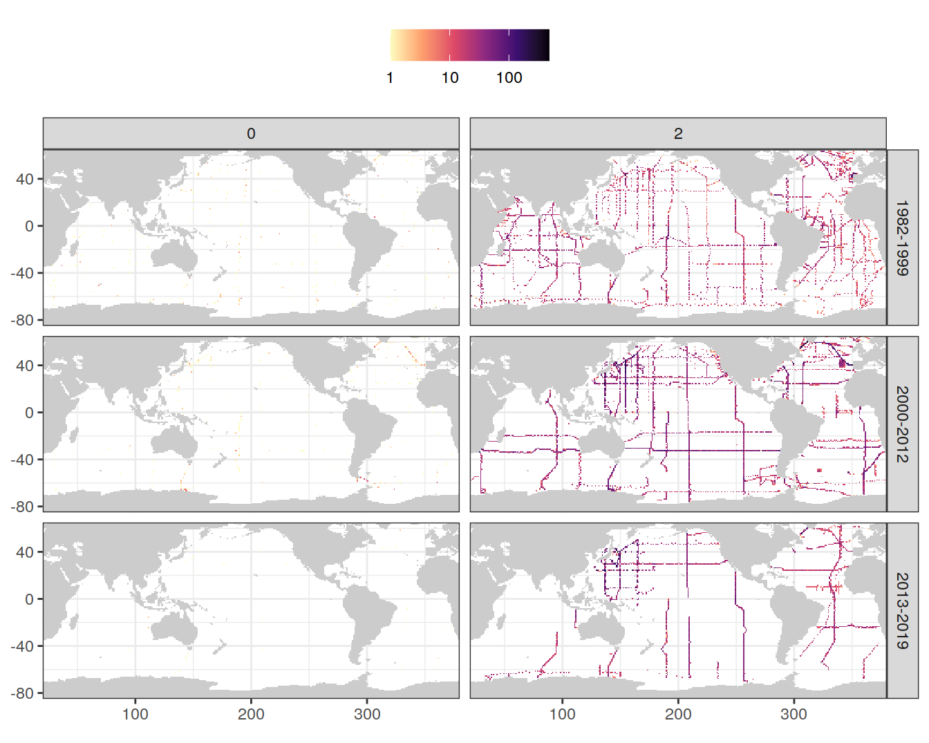
###

GLODAP <- GLODAP %>%
  filter(phosphatef %in% params_local$flag_f)
2.3.3.3 qc flag
GLODAP_obs_grid_temp <- GLODAP %>%
  count(lat, lon, era, phosphateqc)

map +
  geom_raster(data = GLODAP_obs_grid_temp, aes(lon, lat, fill = n)) +
    scale_fill_viridis_c(option = "magma",
                       direction = -1,
                       trans = "log10") +
  facet_grid(era~phosphateqc) +
  theme(legend.position = "top",
        legend.title = element_blank())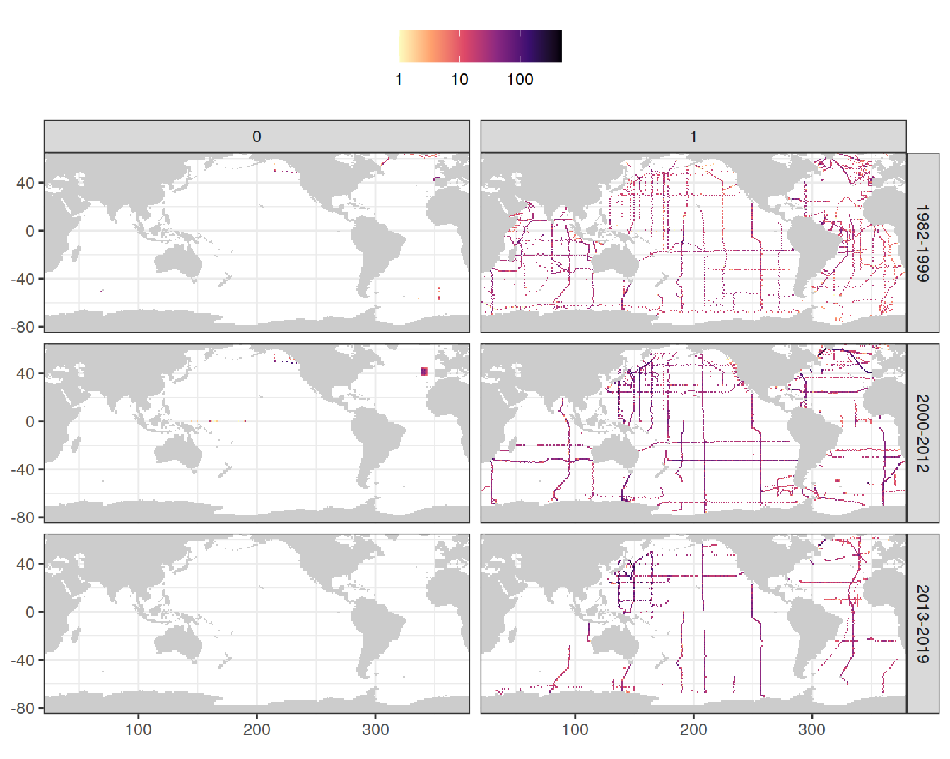
###

GLODAP <- GLODAP %>%
  filter(phosphateqc %in% params_local$flag_qc)

##

GLODAP_stats_temp <- GLODAP %>%
  summarise(phosphate_flag = n())

GLODAP_stats <- cbind(GLODAP_stats, GLODAP_stats_temp)
rm(GLODAP_stats_temp)

##

GLODAP_obs_grid_temp <- GLODAP %>%
  count(lat, lon, era) %>%
  mutate(cleaning_level = "phosphate_flag")

GLODAP_obs_grid <-
  bind_rows(GLODAP_obs_grid, GLODAP_obs_grid_temp)

rm(GLODAP_obs_grid_temp)
2.3.4 eMLR variables
GLODAP <- GLODAP %>%
  filter(!is.na(tem))

##

GLODAP <- GLODAP %>%
  filter(!is.na(sal))

GLODAP <- GLODAP %>%
  filter(salinityf %in% params_local$flag_f)

GLODAP <- GLODAP %>%
  filter(salinityqc %in% params_local$flag_qc)

##

GLODAP <- GLODAP %>%
  filter(!is.na(silicate))

GLODAP <- GLODAP %>%
  filter(silicatef %in% params_local$flag_f)

GLODAP <- GLODAP %>%
  filter(silicateqc %in% params_local$flag_qc)
##

GLODAP <- GLODAP %>%
  filter(!is.na(oxygen))

GLODAP <- GLODAP %>%
  filter(oxygenf %in% params_local$flag_f)

GLODAP <- GLODAP %>%
  filter(oxygenqc %in% params_local$flag_qc)
##

GLODAP <- GLODAP %>%
  filter(!is.na(aou))

GLODAP <- GLODAP %>%
  filter(aouf %in% params_local$flag_f)
##

GLODAP <- GLODAP %>%
  filter(!is.na(nitrate))

GLODAP <- GLODAP %>%
  filter(nitratef %in% params_local$flag_f)

GLODAP <- GLODAP %>%
  filter(nitrateqc %in% params_local$flag_qc)
##

GLODAP <- GLODAP %>%
  filter(!is.na(depth))

GLODAP <- GLODAP %>%
  filter(!is.na(gamma))

##

GLODAP_stats_temp <- GLODAP %>%
  summarise(eMLR_variables = n())

GLODAP_stats <- cbind(GLODAP_stats, GLODAP_stats_temp)

rm(GLODAP_stats_temp)

##

GLODAP_obs_grid_temp <- GLODAP %>%
  count(lat, lon, era) %>%
  mutate(cleaning_level = "eMLR_variables")

GLODAP_obs_grid <-
  bind_rows(GLODAP_obs_grid, GLODAP_obs_grid_temp)

rm(GLODAP_obs_grid_temp)
GLODAP <- GLODAP %>%
select(-ends_with(c("f", "qc")))2.3.5 Manual adjustment A16 cruise
For harmonization with Gruber et al. (2019), cruises 1041 (A16N) and 1042 (A16S) were grouped into the 2000-2012 era despite taking place in 2013/14.
GLODAP_cruises <- GLODAP %>%
  filter(basin == "Atlantic",
         year %in% c(2013, 2014)) %>%
  count(lat, lon, cruise)

map +
  geom_raster(data = GLODAP_cruises, aes(lon, lat, fill = as.factor(cruise))) +
  scale_fill_brewer(palette = "Dark2") +
  theme(legend.position = "top",
        legend.title = element_blank())
| Version | Author | Date |
|---|---|---|
| 196be51 | jens-daniel-mueller | 2020-11-30 |
rm(GLODAP_cruises)GLODAP <- GLODAP %>%
mutate(era = if_else(cruise %in% c(1041, 1042),
sort(unique(GLODAP$era))[2], era))2.4 Create clean observations grid
Grid containing all grid cells where at least one observation remains available after cleaning.
GLODAP_obs_grid_clean <- GLODAP %>%
  count(lat, lon) %>%
  select(-n)
2.5 Write summary file
GLODAP_obs_grid_clean  %>%  write_csv(paste(path_version_data,
                                            "GLODAPv2.2020_clean_obs_grid.csv",
                                            sep = ""))

# select relevant columns for further analysis
GLODAP <- GLODAP %>%
  select(year, date, era, basin, lat, lon, cruise,
         bottomdepth, depth, tem, sal, gamma,
         tco2, talk, phosphate,
         oxygen, aou, nitrate, silicate)


GLODAP  %>%  write_csv(paste(path_version_data,
                             "GLODAPv2.2020_clean.csv",
                             sep = ""))
3 Overview plots
3.1 Cleaning stats
Number of observations at various steps of data cleaning.
GLODAP_stats_long <- GLODAP_stats %>%
  pivot_longer(1:length(GLODAP_stats),
               names_to = "parameter",
               values_to = "n")

GLODAP_stats_long <- GLODAP_stats_long %>%
  mutate(parameter = fct_reorder(parameter, n))

GLODAP_stats_long %>%
  ggplot(aes(parameter, n/1000)) +
  geom_col() +
  coord_flip() +
  labs(y = "n (1000)") +
  theme(axis.title.y = element_blank())
rm(GLODAP_stats_long)3.2 Assign coarse spatial grid
For the following plots, the cleaned data set was re-opened and observations were gridded spatially to intervals of:
- 5° x 5°
GLODAP <- m_grid_horizontal_coarse(GLODAP)3.3 Histogram Zonal coverage
GLODAP_histogram_lat <- GLODAP %>%
  group_by(era, lat_grid, basin) %>%
  tally() %>%
  ungroup()

GLODAP_histogram_lat %>%
  ggplot(aes(lat_grid, n, fill = era)) +
  geom_col() +
  scale_fill_brewer(palette = "Dark2") +
  facet_wrap( ~ basin) +
  coord_flip(expand = 0) +
  theme(legend.position = "top",
        legend.title = element_blank())
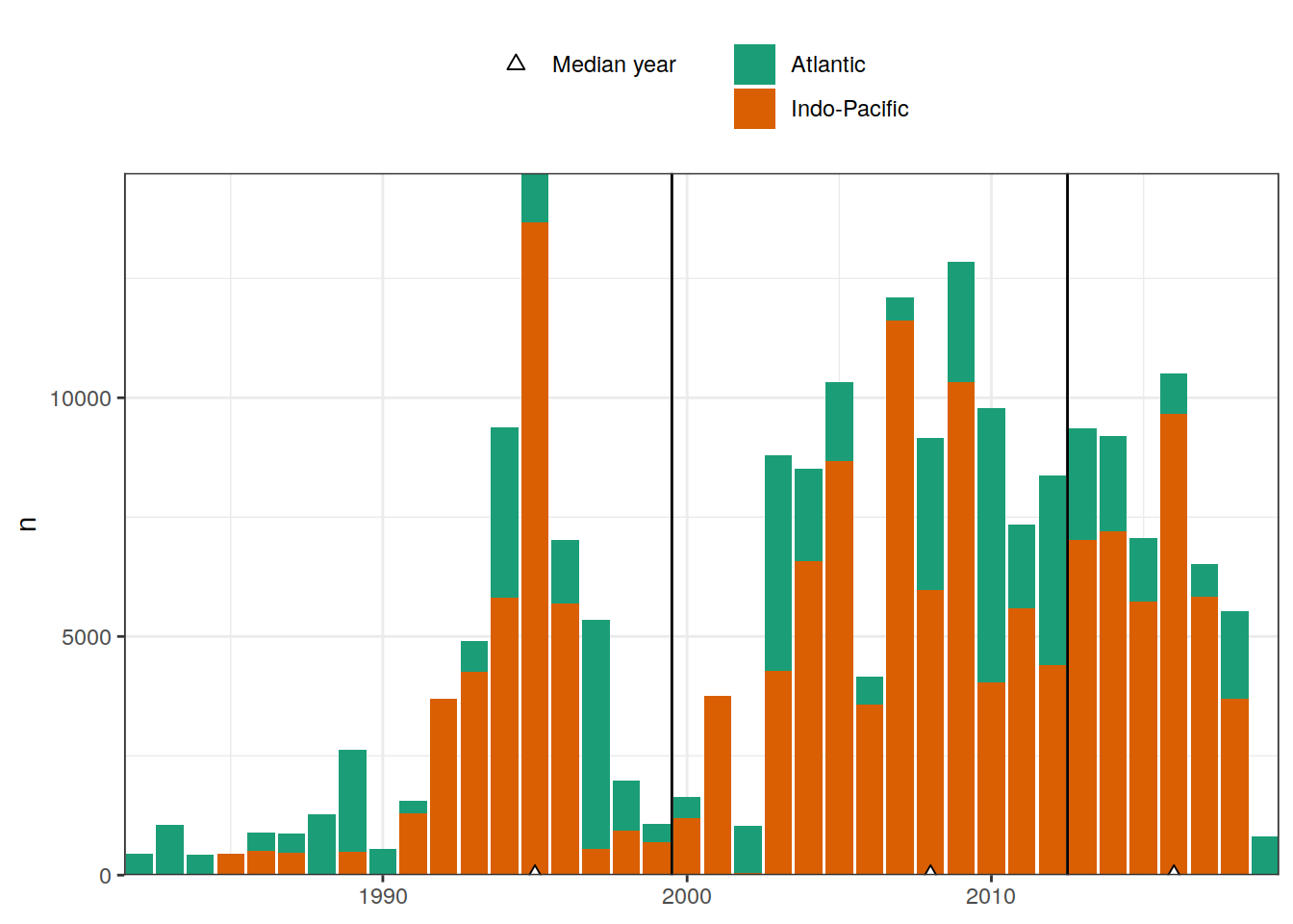
rm(GLODAP_histogram_lat)3.4 Histogram temporal coverage
GLODAP_histogram_year <- GLODAP %>%
  group_by(year, basin) %>%
  tally() %>%
  ungroup()

era_median_year <- GLODAP %>%
  group_by(era) %>%
  summarise(t_ref = median(year)) %>%
  ungroup()

era_median_year
# A tibble: 3 x 2
era t_ref
<fct> <dbl>
1 1982-1999 1995
2 2000-2012 2008
3 2013-2019 2016GLODAP_histogram_year %>%
ggplot() +
geom_vline(xintercept = c(
params_local$era_breaks + 0.5
)) +
geom_col(aes(year, n, fill = basin)) +
geom_point(
data = era_median_year,
aes(t_ref, 0, shape = "Median year"),
size = 2,
fill = "white"
) +
scale_fill_brewer(palette = "Dark2") +
scale_shape_manual(values = 24, name = "") +
scale_y_continuous() +
coord_cartesian(expand = 0) +
theme(
legend.position = "top",
legend.direction = "vertical",
legend.title = element_blank(),
axis.title.x = element_blank()
)
rm(GLODAP_histogram_year,
   era_median_year)
3.5 Zonal temporal coverage (Hovmoeller)
GLODAP_hovmoeller_year <- GLODAP %>%
  group_by(year, lat_grid, basin) %>%
  tally() %>%
  ungroup()

GLODAP_hovmoeller_year %>%
  ggplot(aes(year, lat_grid, fill = n)) +
  geom_tile() +
  geom_vline(xintercept = c(1999.5, 2012.5)) +
  scale_fill_viridis_c(option = "magma",
                       direction = -1,
                       trans = "log10") +
  facet_wrap( ~ basin, ncol = 1) +
  theme(legend.position = "top",
        axis.title.x = element_blank())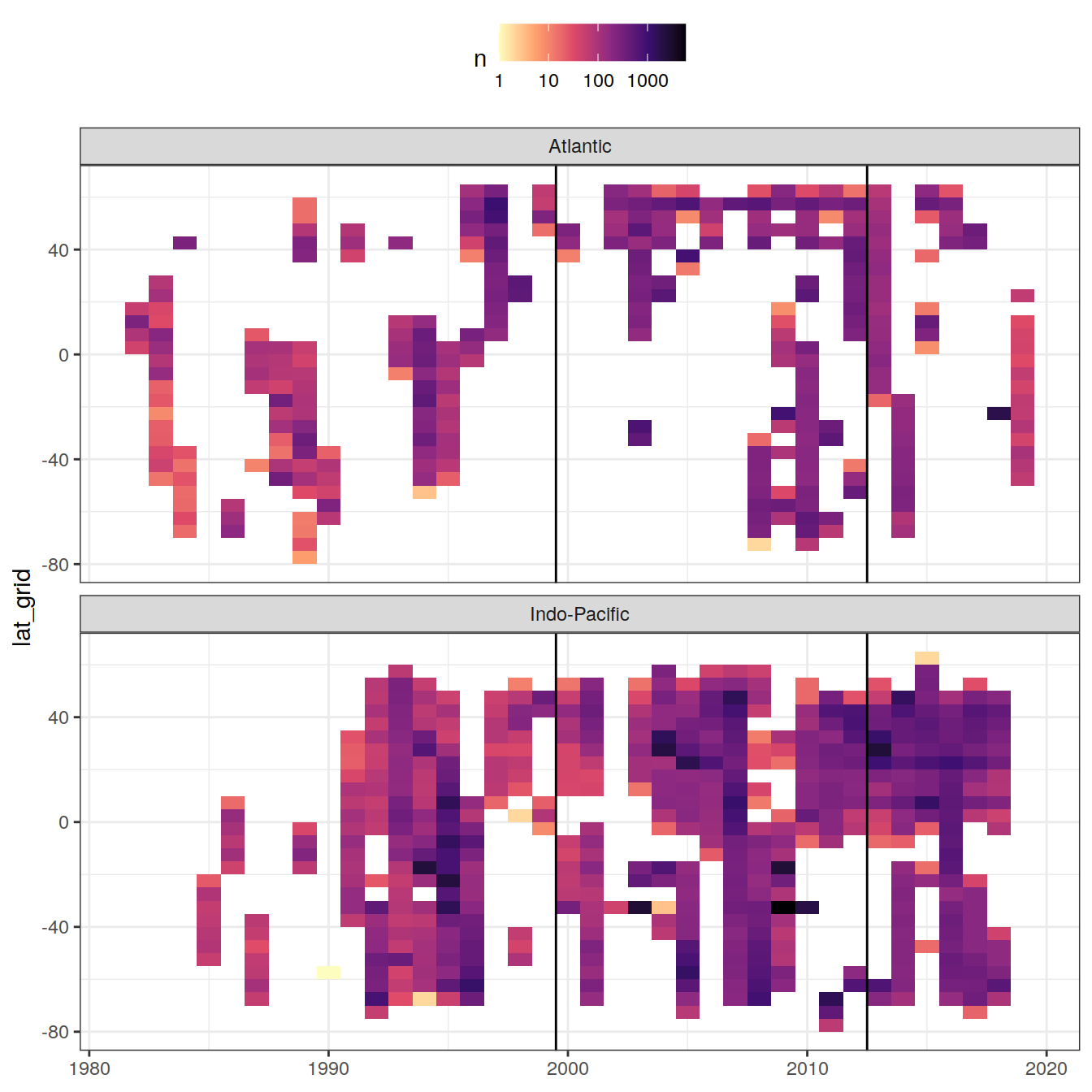
rm(GLODAP_hovmoeller_year)3.6 Coverage maps by era
3.6.1 Subsetting process
The following plots show the remaining data after several cleaning steps, separately for each era.
GLODAP_obs_grid <- GLODAP_obs_grid %>%
  mutate(cleaning_level = factor(
           cleaning_level,
           unique(GLODAP_obs_grid$cleaning_level)
         ))

map +
  geom_raster(data = GLODAP_obs_grid %>%
                filter(cleaning_level == "tco2_values") %>%
                select(-cleaning_level),
              aes(lon, lat, fill = "tco2_values")) +
  geom_raster(data = GLODAP_obs_grid %>%
                filter(cleaning_level != "tco2_values"),
              aes(lon, lat, fill = "subset")) +
  scale_fill_brewer(palette = "Set1", name = "") +
  facet_grid(cleaning_level ~ era) +
  theme(legend.position = "top",
        axis.title = element_blank())
3.6.2 Final input data
The following plots show the remaining data density in each grid cell after all cleaning steps, separately for each era.
GLODAP_tco2_grid <- GLODAP %>%
  count(lat, lon)

map +
  # geom_raster(data = GLODAP_tco2_grid, aes(lon, lat), fill = "grey80") +
  geom_bin2d(data = GLODAP,
             aes(lon, lat),
             binwidth = c(1,1)) +
  scale_fill_viridis_c(option = "magma", direction = -1, trans = "log10") +
  facet_wrap(~era, ncol = 1) +
  labs(title = "Cleaned GLODAP observations",
       subtitle = paste("Version:", params_local$Version_ID)) +
  theme(axis.title = element_blank())
ggsave(path = path_version_figures,
       filename = "data_distribution_era.png",
       height = 8,
       width = 5)
sessionInfo()R version 4.0.3 (2020-10-10)
Platform: x86_64-pc-linux-gnu (64-bit)
Running under: openSUSE Leap 15.1
Matrix products: default
BLAS: /usr/local/R-4.0.3/lib64/R/lib/libRblas.so
LAPACK: /usr/local/R-4.0.3/lib64/R/lib/libRlapack.so
locale:
[1] LC_CTYPE=en_US.UTF-8 LC_NUMERIC=C
[3] LC_TIME=en_US.UTF-8 LC_COLLATE=en_US.UTF-8
[5] LC_MONETARY=en_US.UTF-8 LC_MESSAGES=en_US.UTF-8
[7] LC_PAPER=en_US.UTF-8 LC_NAME=C
[9] LC_ADDRESS=C LC_TELEPHONE=C
[11] LC_MEASUREMENT=en_US.UTF-8 LC_IDENTIFICATION=C
attached base packages:
[1] stats graphics grDevices utils datasets methods base
other attached packages:
[1] lubridate_1.7.9 metR_0.9.0 scico_1.2.0 patchwork_1.1.0
[5] collapse_1.4.2 forcats_0.5.0 stringr_1.4.0 dplyr_1.0.2
[9] purrr_0.3.4 readr_1.4.0 tidyr_1.1.2 tibble_3.0.4
[13] ggplot2_3.3.2 tidyverse_1.3.0 workflowr_1.6.2
loaded via a namespace (and not attached):
[1] httr_1.4.2 jsonlite_1.7.1 viridisLite_0.3.0
[4] here_0.1 modelr_0.1.8 assertthat_0.2.1
[7] blob_1.2.1 cellranger_1.1.0 yaml_2.2.1
[10] pillar_1.4.7 backports_1.1.10 lattice_0.20-41
[13] glue_1.4.2 RcppEigen_0.3.3.7.0 digest_0.6.27
[16] RColorBrewer_1.1-2 promises_1.1.1 checkmate_2.0.0
[19] rvest_0.3.6 colorspace_2.0-0 htmltools_0.5.0
[22] httpuv_1.5.4 Matrix_1.2-18 pkgconfig_2.0.3
[25] broom_0.7.2 haven_2.3.1 scales_1.1.1
[28] whisker_0.4 later_1.1.0.1 git2r_0.27.1
[31] generics_0.0.2 farver_2.0.3 ellipsis_0.3.1
[34] withr_2.3.0 cli_2.2.0 magrittr_2.0.1
[37] crayon_1.3.4 readxl_1.3.1 evaluate_0.14
[40] fs_1.5.0 fansi_0.4.1 xml2_1.3.2
[43] RcppArmadillo_0.10.1.2.0 tools_4.0.3 data.table_1.13.2
[46] hms_0.5.3 lifecycle_0.2.0 munsell_0.5.0
[49] reprex_0.3.0 compiler_4.0.3 rlang_0.4.9
[52] grid_4.0.3 rstudioapi_0.13 labeling_0.4.2
[55] rmarkdown_2.5 gtable_0.3.0 DBI_1.1.0
[58] R6_2.5.0 knitr_1.30 utf8_1.1.4
[61] rprojroot_2.0.2 stringi_1.5.3 parallel_4.0.3
[64] Rcpp_1.0.5 vctrs_0.3.5 dbplyr_1.4.4
[67] tidyselect_1.1.0 xfun_0.18