OceanSODA
Jens Daniel Müller
22 March, 2024
Last updated: 2024-03-22
Checks: 7 0
Knit directory:
heatwave_co2_flux_2023/analysis/
This reproducible R Markdown analysis was created with workflowr (version 1.7.0). The Checks tab describes the reproducibility checks that were applied when the results were created. The Past versions tab lists the development history.
Great! Since the R Markdown file has been committed to the Git repository, you know the exact version of the code that produced these results.
Great job! The global environment was empty. Objects defined in the global environment can affect the analysis in your R Markdown file in unknown ways. For reproduciblity it’s best to always run the code in an empty environment.
The command set.seed(20240307) was run prior to running
the code in the R Markdown file. Setting a seed ensures that any results
that rely on randomness, e.g. subsampling or permutations, are
reproducible.
Great job! Recording the operating system, R version, and package versions is critical for reproducibility.
Nice! There were no cached chunks for this analysis, so you can be confident that you successfully produced the results during this run.
Great job! Using relative paths to the files within your workflowr project makes it easier to run your code on other machines.
Great! You are using Git for version control. Tracking code development and connecting the code version to the results is critical for reproducibility.
The results in this page were generated with repository version f69ff93. See the Past versions tab to see a history of the changes made to the R Markdown and HTML files.
Note that you need to be careful to ensure that all relevant files for
the analysis have been committed to Git prior to generating the results
(you can use wflow_publish or
wflow_git_commit). workflowr only checks the R Markdown
file, but you know if there are other scripts or data files that it
depends on. Below is the status of the Git repository when the results
were generated:
Ignored files:
    Ignored:    .Rhistory
    Ignored:    .Rproj.user/

Unstaged changes:
    Modified:   analysis/child/pCO2_product_analysis.Rmd
    Modified:   code/Workflowr_project_managment.R
Note that any generated files, e.g. HTML, png, CSS, etc., are not included in this status report because it is ok for generated content to have uncommitted changes.
These are the previous versions of the repository in which changes were
made to the R Markdown (analysis/OceanSODA.Rmd) and HTML
(docs/OceanSODA.html) files. If you’ve configured a remote
Git repository (see ?wflow_git_remote), click on the
hyperlinks in the table below to view the files as they were in that
past version.
| File | Version | Author | Date | Message |
|---|---|---|---|---|
| html | 98cf341 | jens-daniel-mueller | 2024-03-21 | Build site. |
| html | e3e1491 | jens-daniel-mueller | 2024-03-21 | Build site. |
| html | 47238da | jens-daniel-mueller | 2024-03-21 | Build site. |
| html | 2fdbfec | jens-daniel-mueller | 2024-03-21 | Build site. |
| Rmd | d476020 | jens-daniel-mueller | 2024-03-21 | convert kw unit |
| html | 83fcd67 | jens-daniel-mueller | 2024-03-21 | Build site. |
| html | 342018b | jens-daniel-mueller | 2024-03-20 | Build site. |
| Rmd | 8120865 | jens-daniel-mueller | 2024-03-20 | hovmoeller anomalies not without 2023 data |
| html | f0a1de7 | jens-daniel-mueller | 2024-03-20 | Build site. |
| html | 2d2fb75 | jens-daniel-mueller | 2024-03-20 | Build site. |
| Rmd | 23dde7a | jens-daniel-mueller | 2024-03-20 | new variables added |
| html | 8698b51 | jens-daniel-mueller | 2024-03-20 | Build site. |
| Rmd | 39d9769 | jens-daniel-mueller | 2024-03-20 | write summary output files |
| html | d520917 | jens-daniel-mueller | 2024-03-19 | Build site. |
| Rmd | 3b8f860 | jens-daniel-mueller | 2024-03-19 | solubility and SSS included |
| html | 03321bd | jens-daniel-mueller | 2024-03-19 | Build site. |
| Rmd | e80f0d8 | jens-daniel-mueller | 2024-03-19 | units fixed |
| html | b41fa51 | jens-daniel-mueller | 2024-03-19 | Build site. |
| html | bd3c1fe | jens-daniel-mueller | 2024-03-19 | Build site. |
| Rmd | fbfd936 | jens-daniel-mueller | 2024-03-19 | run pco2 products with child document |
| html | 5c97a86 | jens-daniel-mueller | 2024-03-19 | Build site. |
| Rmd | 60bf95f | jens-daniel-mueller | 2024-03-19 | run OceanSODA with child document |
| html | 604281a | jens-daniel-mueller | 2024-03-19 | Build site. |
| Rmd | 949479e | jens-daniel-mueller | 2024-03-19 | run OceanSODA with child document |
| html | 14a6ce5 | jens-daniel-mueller | 2024-03-19 | Build site. |
| Rmd | cdff298 | jens-daniel-mueller | 2024-03-19 | run OceanSODA with child document |
| html | d3f3f52 | jens-daniel-mueller | 2024-03-18 | Build site. |
| Rmd | c3f5bd6 | jens-daniel-mueller | 2024-03-18 | run OceanSODA with child document |
center <- -160
boundary <- center + 180
target_crs <- paste0("+proj=robin +over +lon_0=", center)
# target_crs <- paste0("+proj=eqearth +over +lon_0=", center)
# target_crs <- paste0("+proj=eqearth +lon_0=", center)
# target_crs <- paste0("+proj=igh_o +lon_0=", center)

worldmap <- ne_countries(scale = 'small',
                         type = 'map_units',
                         returnclass = 'sf')

worldmap <- worldmap %>% st_break_antimeridian(lon_0 = center)
worldmap_trans <- st_transform(worldmap, crs = target_crs)

# ggplot() +
#   geom_sf(data = worldmap_trans)

coastline <- ne_coastline(scale = 'small', returnclass = "sf")
coastline <- st_break_antimeridian(coastline, lon_0 = 200)
coastline_trans <- st_transform(coastline, crs = target_crs)

# ggplot() +
#   geom_sf(data = worldmap_trans, fill = "grey", col="grey") +
#   geom_sf(data = coastline_trans)


bbox <- st_bbox(c(xmin = -180, xmax = 180, ymax = 65, ymin = -78), crs = st_crs(4326))
bbox <- st_as_sfc(bbox)
bbox_trans <- st_break_antimeridian(bbox, lon_0 = center)

bbox_graticules <- st_graticule(
  x = bbox_trans,
  crs = st_crs(bbox_trans),
  datum = st_crs(bbox_trans),
  lon = c(20, 20.001),
  lat = c(-78,65),
  ndiscr = 1e3,
  margin = 0.001
)

bbox_graticules_trans <- st_transform(bbox_graticules, crs = target_crs)
rm(worldmap, coastline, bbox, bbox_trans)

# ggplot() +
#   geom_sf(data = worldmap_trans, fill = "grey", col="grey") +
#   geom_sf(data = coastline_trans) +
#   geom_sf(data = bbox_graticules_trans)

lat_lim <- ext(bbox_graticules_trans)[c(3,4)]*1.002
lon_lim <- ext(bbox_graticules_trans)[c(1,2)]*1.005

# ggplot() +
#   geom_sf(data = worldmap_trans, fill = "grey90", col = "grey90") +
#   geom_sf(data = coastline_trans) +
#   geom_sf(data = bbox_graticules_trans, linewidth = 1) +
#   coord_sf(crs = target_crs,
#            ylim = lat_lim,
#            xlim = lon_lim,
#            expand = FALSE) +
#   theme(
#     panel.border = element_blank(),
#     axis.text = element_blank(),
#     axis.ticks = element_blank()
#   )

latitude_graticules <- st_graticule(
  x = bbox_graticules,
  crs = st_crs(bbox_graticules),
  datum = st_crs(bbox_graticules),
  lon = c(20, 20.001),
  lat = c(-60,-30,0,30,60),
  ndiscr = 1e3,
  margin = 0.001
)

latitude_graticules_trans <- st_transform(latitude_graticules, crs = target_crs)

latitude_labels <- data.frame(lat_label = c("60°N","30°N","Eq.","30°S","60°S"),
                 lat = c(60,30,0,-30,-60)-4, lon = c(35)-c(0,2,4,2,0))

latitude_labels <- st_as_sf(x = latitude_labels,
               coords = c("lon", "lat"),
               crs = "+proj=longlat")

latitude_labels_trans <- st_transform(latitude_labels, crs = target_crs)

# ggplot() +
#   geom_sf(data = worldmap_trans, fill = "grey", col = "grey") +
#   geom_sf(data = coastline_trans) +
#   geom_sf(data = bbox_graticules_trans) +
#   geom_sf(data = latitude_graticules_trans,
#           col = "grey60",
#           linewidth = 0.2) +
#   geom_sf_text(data = latitude_labels_trans,
#                aes(label = lat_label),
#                size = 3,
#                col = "grey60")
Read data
path_pCO2_products <-
  "/nfs/kryo/work/datasets/gridded/ocean/2d/observation/pco2/"

path_OceanSODA <-
  "/nfs/kryo/work/gregorl/projects/OceanSODA-ETHZ/releases/v2023-full_carbonate_system/OceanSODA_ETHZ_HRLR-v2023.01-co2fluxvars-netCDF/"
library(ncdf4)
nc <-
nc_open(paste0(
path_pCO2_products,
"VLIZ-SOM_FFN/VLIZ-SOM_FFN_vBAMS2024.nc"
))
nc <-
nc_open(paste0(
path_OceanSODA,
"kw_OceanSODA_ETHZ_HR_LR-v2023.01-1982_2023.nc"
))
print(nc)OceanSODA_files <- list.files(path = path_OceanSODA)
OceanSODA_files <-
OceanSODA_files[OceanSODA_files %>% str_detect(c("mld|press|chl"))]
for (i_OceanSODA_files in OceanSODA_files) {
# i_OceanSODA_files <- OceanSODA_files[2]
i_pco2_product <-
read_ncdf(paste0(path_OceanSODA,
i_OceanSODA_files),
make_units = FALSE,
ignore_bounds = TRUE)
if (exists("pco2_product")) {
pco2_product <-
c(pco2_product,
i_pco2_product)
}
if (!exists("pco2_product")) {
pco2_product <- i_pco2_product
}
}
rm(OceanSODA_files, i_OceanSODA_files, i_pco2_product)
pco2_product <- pco2_product %>%
as_tibble()
pco2_product_temp <- pco2_product
rm(pco2_product)
# pco2_product_temp %>%
# # mutate(chl_filled = 10^chl_filled) %>%
# # filter(chl_filled < 5) %>%
# ggplot(aes(chl_filled)) +
# geom_histogram()
OceanSODA_files <- list.files(path = path_OceanSODA)
OceanSODA_files <-
OceanSODA_files[OceanSODA_files %>% str_detect(c("dfco2|fgco2_O|kw|spco2|temp|sal|sol"))]
for (i_OceanSODA_files in OceanSODA_files) {
# i_OceanSODA_files <- OceanSODA_files[2]
i_pco2_product <-
read_ncdf(paste0(path_OceanSODA,
i_OceanSODA_files),
make_units = FALSE,
ignore_bounds = TRUE)
if (exists("pco2_product")) {
pco2_product <-
c(pco2_product,
i_pco2_product)
}
if (!exists("pco2_product")) {
pco2_product <- i_pco2_product
}
}
rm(OceanSODA_files, i_OceanSODA_files, i_pco2_product)
# rm(pco2_product)
pco2_product <- pco2_product %>%
as_tibble()
pco2_product <-
full_join(pco2_product, pco2_product_temp)
rm(pco2_product_temp)
pco2_product <-
pco2_product %>%
mutate(area = earth_surf(lat, lon),
year = year(time),
month = month(time))
pco2_product <-
pco2_product %>%
mutate(lon = if_else(lon < 20, lon + 360, lon),
fgco2 = fgco2 * 1e-3 * 365,
sol = sol * 1e-3,
mld = 10^mld,
chl_filled = 10^chl_filled,
kw = kw * 1e-2 * 24 * 365) %>%
rename(chl = chl_filled)pCO2productanalysis <-
knitr::knit_expand(
file = here::here("analysis/child/pCO2_product_analysis.Rmd"),
product_name = "OceanSODA"
)Read data
path_reccap2 <-
"/nfs/kryo/work/datasets/gridded/ocean/interior/reccap2/"print("RECCAP2_region_masks_all_v20221025.nc")[1] "RECCAP2_region_masks_all_v20221025.nc"biome_mask <-
read_ncdf(
paste(
path_reccap2,
"supplementary/RECCAP2_region_masks_all_v20221025.nc",
sep = ""
)
) %>%
as_tibble()Analysis settings
key_biomes <- c("global",
                "NA-SPSS",
                "NA-STPS",
                "NP-SPSS",
                "PEQU-E",
                "SO-SPSS")

key_biomes %>%
  write_rds("../data/key_biomes.rds")

name_quadratic_fit <- c("atm_co2", "spco2", "sfco2")

start_year <- 1990

name_divergent <- c("dco2", "fgco2", "fgco2_hov", "fgco2_int")
Anomaly detection
For the detection of anomalies at any point in time and space, we fit regression models and compare the fitted to the actual value.
We use linear regression models for all parameters, except for `, which are approximated with quadratic fits.
The regression models are fitted to data from the period `, and extrapolated to 2023.
anomaly_determination <- function(df,...) {

  group_by <- quos(...)

  # Linear regression models

  df_lm <-
    df %>%
    filter(year <= 2022,
           !(name %in% name_quadratic_fit)) %>%
    nest(data = -c(name, !!!group_by)) %>%
    mutate(
      fit = map(data, ~ lm(value ~ year, data = .x)),
      tidied = map(fit, tidy),
      augmented = map(fit, augment)
    )


  df_lm_2023 <-
    full_join(
      df_lm %>%
        unnest(tidied) %>%
        select(name, !!!group_by, term, estimate) %>%
        pivot_wider(names_from = term,
                    values_from = estimate) %>%
        mutate(fit = `(Intercept)` + year * 2023) %>%
        select(name, !!!group_by, fit) %>%
        mutate(year = 2023),
      df %>%
        filter(year == 2023,
               !(name %in% name_quadratic_fit))
    ) %>%
    mutate(resid = value - fit)


  df_lm <-
    bind_rows(
      df_lm %>%
        unnest(augmented) %>%
        select(name, !!!group_by, year, value, fit = .fitted, resid = .resid),
      df_lm_2023
    )

  rm(df_lm_2023)

  # Quadratic regression models

  df_quadratic <-
    df %>%
    filter(year <= 2022,
           name %in% name_quadratic_fit) %>%
    nest(data = -c(name, !!!group_by)) %>%
    mutate(
      fit = map(data, ~ lm(value ~ year + I(year ^ 2), data = .x)),
      tidied = map(fit, tidy),
      augmented = map(fit, augment)
    )


  df_quadratic_2023 <-
    full_join(
      df_quadratic %>%
        unnest(tidied) %>%
        select(name, !!!group_by, term, estimate) %>%
        pivot_wider(names_from = term,
                    values_from = estimate) %>%
        mutate(fit = `(Intercept)` + year * 2023 + `I(year^2)` * 2023 ^ 2) %>%
        select(name, !!!group_by, fit) %>%
        mutate(year = 2023),
      df %>%
        filter(year == 2023,
               name %in% name_quadratic_fit)
    ) %>%
    mutate(resid = value - fit)


  df_quadratic <-
    bind_rows(
      df_quadratic %>%
        unnest(augmented) %>%
        select(name, !!!group_by, year, value, fit = .fitted, resid = .resid),
      df_quadratic_2023
    )

  rm(df_quadratic_2023)

  # Join linear and quadratic regression results

  df_regression <-
    bind_rows(df_lm,
              df_quadratic)

  rm(df_lm,
     df_quadratic)


  return(df_regression)

}
Biome mask
biome_mask <-
  biome_mask %>%
  mutate(lon = if_else(lon < 20, lon + 360, lon))

land_mask <- biome_mask %>%
  filter(seamask == 0) %>%
  select(lon, lat)

map <- ggplot(land_mask,
              aes(lon, lat)) +
  geom_tile(fill = "grey80") +
  scale_y_continuous(breaks = seq(-60,60,30)) +
  scale_x_continuous(breaks = seq(0,360,60)) +
  coord_quickmap(expand = 0, ylim = c(-80, 80)) +
  theme(axis.title = element_blank(),
        axis.text = element_blank(),
        axis.ticks = element_blank())

map %>%
  write_rds("../data/map.rds")

biome_mask <- biome_mask %>%
  filter(seamask == 1) %>%
  select(lon, lat, atlantic:southern) %>%
  pivot_longer(atlantic:southern,
               names_to = "region",
               values_to = "biome") %>%
  mutate(biome = as.character(biome))

biome_mask <- biome_mask %>%
  filter(biome != "0")

biome_mask <- biome_mask %>%
  mutate(biome = paste(region, biome, sep = "_"))

biome_mask <- biome_mask  %>%
  mutate(biome = case_when(
    biome == "atlantic_1" ~ "NA-SPSS",
    biome == "atlantic_2" ~ "NA-STSS",
    biome == "atlantic_3" ~ "NA-STPS",
    biome == "atlantic_4" ~ "AEQU",
    biome == "atlantic_5" ~ "SA-STPS",
    # biome == "atlantic_6" ~ "MED",
    biome == "pacific_1" ~ "NP-SPSS",
    biome == "pacific_2" ~ "NP-STSS",
    biome == "pacific_3" ~ "NP-STPS",
    biome == "pacific_4" ~ "PEQU-W",
    biome == "pacific_5" ~ "PEQU-E",
    biome == "pacific_6" ~ "SP-STSS",
    biome == "indian_1" ~ "Arabian Sea",
    biome == "indian_2" ~ "Bay of Bengal",
    biome == "indian_3" ~ "Equatorial Indian",
    biome == "indian_4" ~ "Southern Indian",
    # biome == "arctic_1" ~ "ARCTIC-ICE",
    # biome == "arctic_2" ~ "NP-ICE",
    # biome == "arctic_3" ~ "NA-ICE",
    # biome == "arctic_4" ~ "Barents",
    # str_detect(biome, "arctic") ~ "Arctic",
    biome == "southern_1" ~ "SO-STSS",
    biome == "southern_2" ~ "SO-SPSS",
    # biome == "southern_3" ~ "SO-ICE",
    TRUE ~ "other"
  ))

biome_mask <-
  biome_mask %>%
  filter(biome != "other")

map +
  geom_tile(data = biome_mask,
            aes(lon, lat, fill = region)) +
  labs(title = "Considered ocean regions") +
  scale_fill_muted() +
  theme(legend.title = element_blank())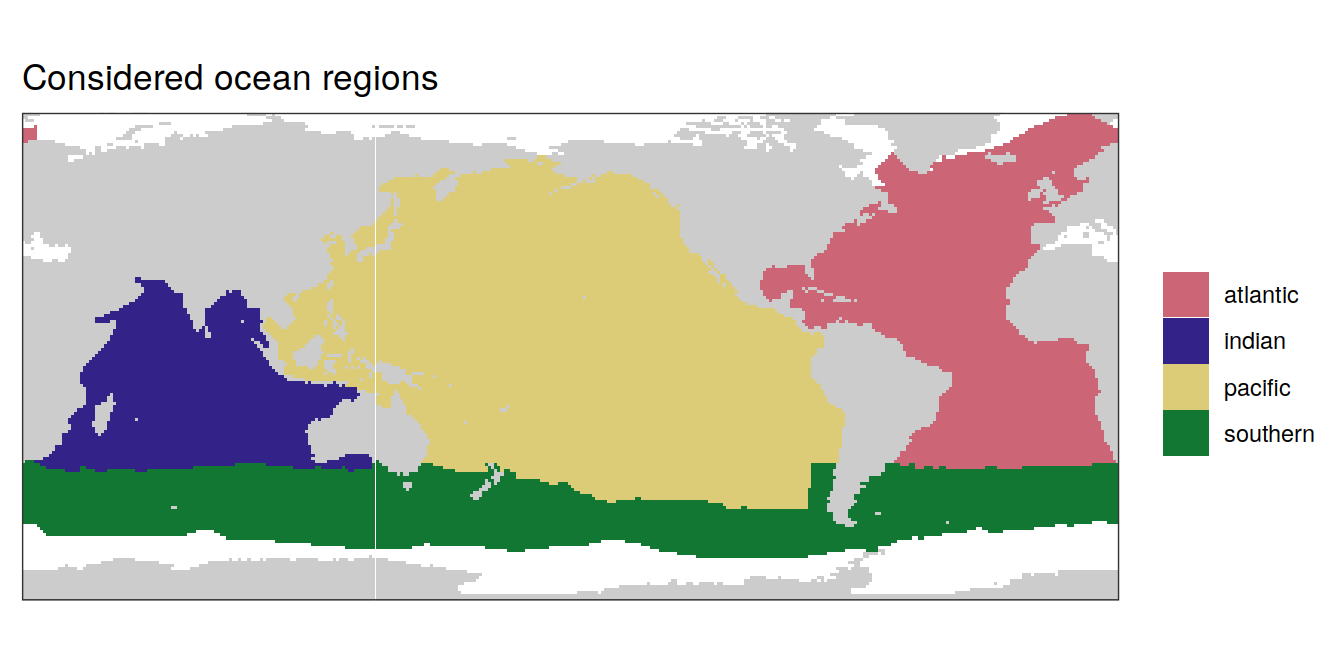
| Version | Author | Date |
|---|---|---|
| b41fa51 | jens-daniel-mueller | 2024-03-19 |
biome_mask %>%
  group_split(region) %>%
  # head(1) %>%
  map( ~ map +
         geom_tile(data = .x,
                   aes(lon, lat, fill = biome)) +
         labs(title = paste("Region:", .x$region)) +
         scale_fill_okabeito())
[[1]]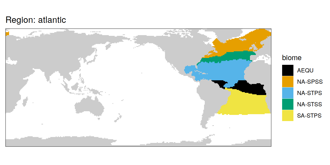
| Version | Author | Date |
|---|---|---|
| b41fa51 | jens-daniel-mueller | 2024-03-19 |
[[2]]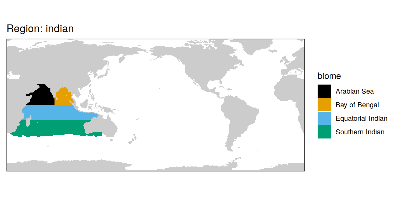
| Version | Author | Date |
|---|---|---|
| b41fa51 | jens-daniel-mueller | 2024-03-19 |
[[3]]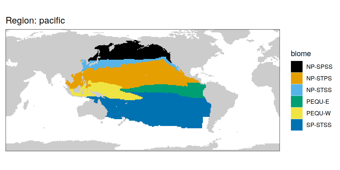
| Version | Author | Date |
|---|---|---|
| b41fa51 | jens-daniel-mueller | 2024-03-19 |
[[4]]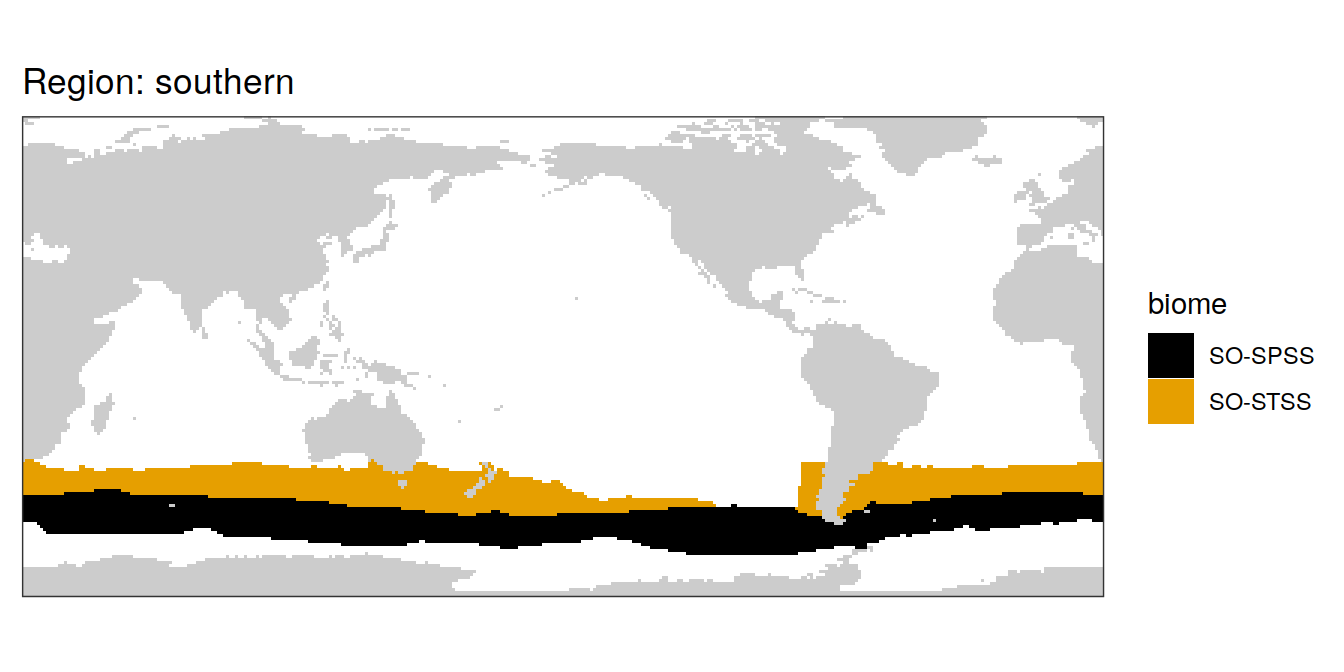
| Version | Author | Date |
|---|---|---|
| b41fa51 | jens-daniel-mueller | 2024-03-19 |
map +
  geom_tile(data = biome_mask %>% filter(biome %in% key_biomes),
            aes(lon, lat, fill = biome)) +
  labs(title = "Selected biomes to highlight") +
  scale_fill_muted() +
  theme(legend.title = element_blank())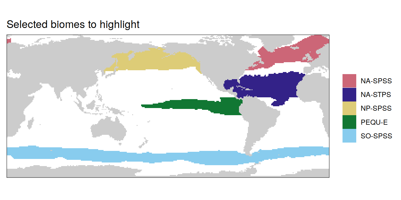
| Version | Author | Date |
|---|---|---|
| b41fa51 | jens-daniel-mueller | 2024-03-19 |
biome_mask <-
  biome_mask %>%
  select(-region)


super_biome_mask <- biome_mask  %>%
  mutate(
    biome = case_when(
      str_detect(biome, "NA-") ~ "North Atlantic",
      str_detect(biome, "NP-") ~ "North Pacific",
      str_detect(biome, "SO-") ~ "Southern Ocean",
      TRUE ~ "other"
    )
  )

super_biome_mask <-
  super_biome_mask %>%
  filter(biome != "other")

map +
  geom_tile(data = super_biome_mask,
            aes(lon, lat, fill = biome)) +
  labs(title = "Selected super biomes") +
  scale_fill_muted() +
  theme(legend.title = element_blank())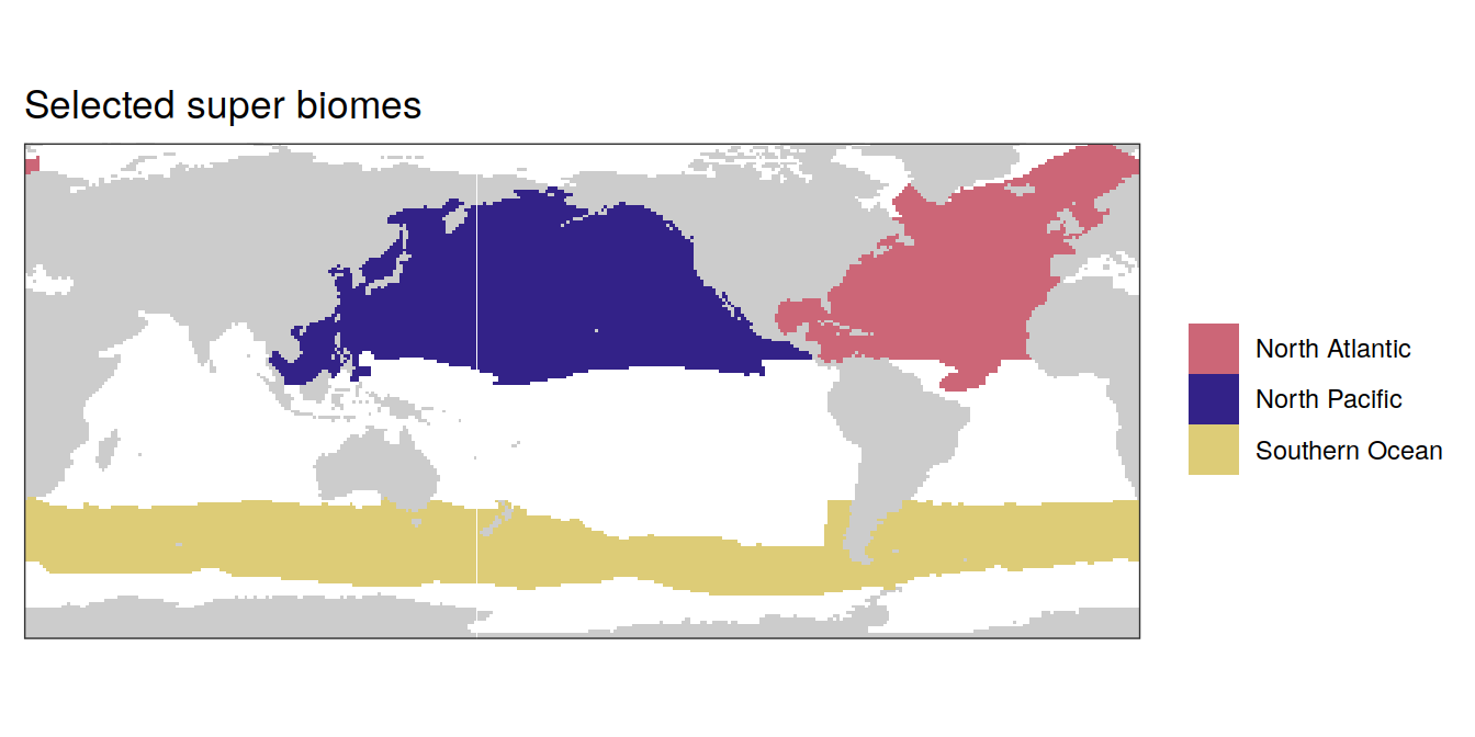
| Version | Author | Date |
|---|---|---|
| e3e1491 | jens-daniel-mueller | 2024-03-21 |
super_biomes <-
  super_biome_mask %>%
  distinct(biome) %>%
  pull()

super_biomes %>%
  write_rds("../data/super_biomes.rds")
Define labels and breaks
labels_breaks <- function(i_name) {

  if (i_name == "dco2") {
    i_legend_title <- "ΔpCO<sub>2</sub><br>(µatm)"
    # i_breaks <- c(-Inf, seq(0, 80, 10), Inf)
    # i_contour_level <- 50
    # i_contour_level_abs <- 2200
  }

  if (i_name == "dfco2") {
    i_legend_title <- "ΔfCO<sub>2</sub><br>(µatm)"
    # i_breaks <- c(-Inf, seq(0, 80, 10), Inf)
    # i_contour_level <- 50
    # i_contour_level_abs <- 2200
  }

  if (i_name == "atm_co2") {
    i_legend_title <- "pCO<sub>2,atm</sub><br>(µatm)"
    # i_breaks <- c(-Inf, seq(0, 80, 10), Inf)
    # i_contour_level <- 50
    # i_contour_level_abs <- 2200
  }

  if (i_name == "sol") {
    i_legend_title <- "CO<sub>2</sub> solubility<br>(mol m<sup>-3</sup> µatm<sup>-1</sup>)"
    # i_breaks <- c(-Inf, seq(0, 80, 10), Inf)
    # i_contour_level <- 50
    # i_contour_level_abs <- 2200
  }

  if (i_name == "kw") {
    i_legend_title <- "K<sub>w</sub><br>(m yr<sup>-1</sup>)"
    # i_breaks <- c(-Inf, seq(0, 80, 10), Inf)
    # i_contour_level <- 50
    # i_contour_level_abs <- 2200
  }

  if (i_name == "spco2") {
    i_legend_title <- "pCO<sub>2,ocean</sub><br>(µatm)"
    # i_breaks <- c(-Inf, seq(0, 80, 10), Inf)
    # i_contour_level <- 50
    # i_contour_level_abs <- 2200
  }

  if (i_name == "sfco2") {
    i_legend_title <- "fCO<sub>2,ocean</sub><br>(µatm)"
    # i_breaks <- c(-Inf, seq(0, 80, 10), Inf)
    # i_contour_level <- 50
    # i_contour_level_abs <- 2200
  }

  if (i_name == "fgco2") {
    i_legend_title <- "FCO<sub>2</sub><br>(mol m<sup>-2</sup> yr<sup>-1</sup>)"
    # i_breaks <- c(-Inf, seq(0, 80, 10), Inf)
    # i_contour_level <- 50
    # i_contour_level_abs <- 2200
  }

  if (i_name == "fgco2_hov") {
    i_legend_title <- "FCO<sub>2</sub><br>(PgC deg<sup>-1</sup> yr<sup>-1</sup>)"
    # i_breaks <- c(-Inf, seq(0, 80, 10), Inf)
    # i_contour_level <- 50
    # i_contour_level_abs <- 2200
  }

  if (i_name == "fgco2_int") {
    i_legend_title <- "FCO<sub>2</sub><br>(PgC yr<sup>-1</sup>)"
    # i_breaks <- c(-Inf, seq(0, 80, 10), Inf)
    # i_contour_level <- 50
    # i_contour_level_abs <- 2200
  }

  if (i_name == "temperature") {
    i_legend_title <- "SST<br>(°C)"
    # i_breaks <- c(-Inf, seq(0, 80, 10), Inf)
    # i_contour_level <- 50
    # i_contour_level_abs <- 2200
  }

  if (i_name == "salinity") {
    i_legend_title <- "SSS"
    # i_breaks <- c(-Inf, seq(0, 80, 10), Inf)
    # i_contour_level <- 50
    # i_contour_level_abs <- 2200
  }

  if (i_name == "chl") {
    i_legend_title <- "Chl-a<br>(mg m<sup>-3</sup>)"
    # i_breaks <- c(-Inf, seq(0, 80, 10), Inf)
    # i_contour_level <- 50
    # i_contour_level_abs <- 2200
  }

  if (i_name == "mld") {
    i_legend_title <- "MLD<br>(m)"
    # i_breaks <- c(-Inf, seq(0, 80, 10), Inf)
    # i_contour_level <- 50
    # i_contour_level_abs <- 2200
  }

  if (i_name == "press") {
    i_legend_title <- "pressure<sub>atm</sub><br>(unit?)"
    # i_breaks <- c(-Inf, seq(0, 80, 10), Inf)
    # i_contour_level <- 50
    # i_contour_level_abs <- 2200
  }

  all_labels_breaks <- lst(i_legend_title,
                           # i_breaks,
                           # i_contour_level,
                           # i_contour_level_abs
                           )

  return(all_labels_breaks)

}


# labels_breaks("fgco2")

x_axis_labels <-
  c(
    "dco2" = labels_breaks("dco2")$i_legend_title,
    "dfco2" = labels_breaks("dfco2")$i_legend_title,
    "atm_co2" = labels_breaks("atm_co2")$i_legend_title,
    "sol" = labels_breaks("sol")$i_legend_title,
    "kw" = labels_breaks("kw")$i_legend_title,
    "spco2" = labels_breaks("spco2")$i_legend_title,
    "sfco2" = labels_breaks("sfco2")$i_legend_title,
    "fgco2_hov" = labels_breaks("fgco2_hov")$i_legend_title,
    "fgco2_int" = labels_breaks("fgco2_int")$i_legend_title,
    "temperature" = labels_breaks("temperature")$i_legend_title,
    "salinity" = labels_breaks("salinity")$i_legend_title,
    "chl" = labels_breaks("chl")$i_legend_title,
    "mld" = labels_breaks("mld")$i_legend_title,
    "press" = labels_breaks("press")$i_legend_title
  )
Preprocessing
pco2_product <-
  pco2_product %>%
  filter(year >= start_year)
pco2_product <-
full_join(pco2_product,
biome_mask)
# set all values outside biome mask to NA
pco2_product <-
pco2_product %>%
mutate(across(-c(lat, lon, time, area, year, month, biome),
~ if_else(is.na(biome), NA, .)))
# map +
# geom_tile(data = pco2_product %>% filter(time == max(time),
# !is.na(fgco2)),
# aes(lon, lat))Maps
The following maps show the absolute state of each variable in 2023 as provided through the pCO2 product, the change in that variable from 1990 to 2023, as well es the anomalies in 2023. Changes and anomalies are determined based on the predicted value of a linear regression model fit to the data from 1990 to 2022.
Maps are first presented as annual means, and than as monthly means. Note that the 2023 predictions for the monthly maps are done individually for each month, such the mean seasonal anomaly from the annual mean is removed.
Note: The increase the computational speed, I regridded all maps to 5X5° grid.
pco2_product_coarse <-
  m_grid_horizontal_coarse(pco2_product)

# pco2_product_coarse %>%
#   distinct(year)

pco2_product_coarse <-
  pco2_product_coarse %>%
  select(-c(lon, lat, time, biome)) %>%
  group_by(year, month, lon_grid, lat_grid) %>%
  summarise(across(-area,
                   ~ weighted.mean(., area))) %>%
  ungroup() %>%
  rename(lon = lon_grid, lat = lat_grid)

pco2_product_coarse <-
  pco2_product_coarse %>%
  pivot_longer(-c(year, month, lon, lat)) %>%
  drop_na() %>%
  pivot_wider()
Annual means
2023 absolute
pco2_product_coarse_annual <-
  pco2_product_coarse %>%
  select(-month) %>%
  group_by(year, lon, lat) %>%
  summarise(across(where(is.numeric),
                   ~ mean(.))) %>%
  ungroup()

pco2_product_coarse_annual <-
  pco2_product_coarse_annual %>%
  pivot_longer(-c(year, lon, lat))


pco2_product_coarse_annual_regression <-
  pco2_product_coarse_annual %>%
  anomaly_determination(lon, lat)

pco2_product_coarse_annual_regression <-
  pco2_product_coarse_annual_regression %>%
  drop_na()

pco2_product_coarse_annual_regression %>%
  filter(year == 2023,
         !(name %in% name_divergent)) %>%
  group_split(name) %>%
  # head(1) %>%
  map(
    ~ map +
      geom_tile(data = .x,
                aes(lon, lat, fill = value)) +
      labs(title = "Annual mean 2023") +
      scale_fill_viridis_c(name = labels_breaks(.x %>% distinct(name))) +
      theme(legend.title = element_markdown())
  )
[[1]]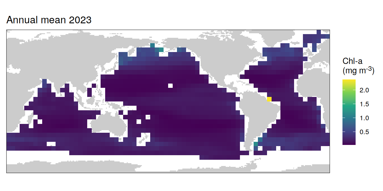
[[2]]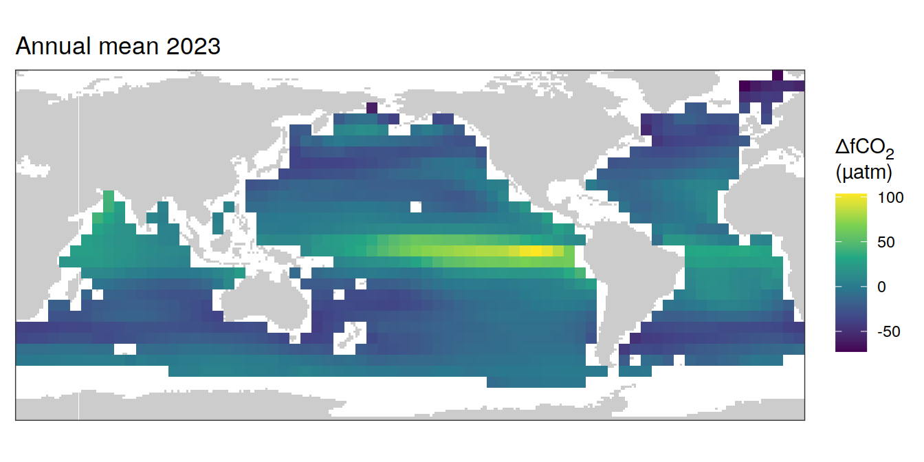
[[3]]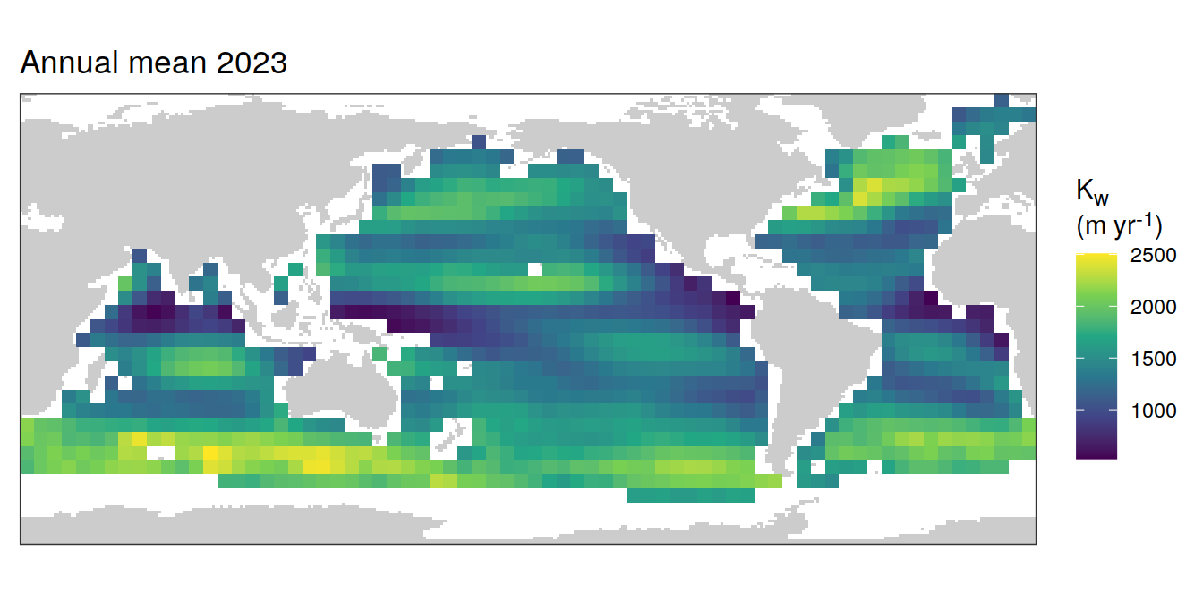
[[4]]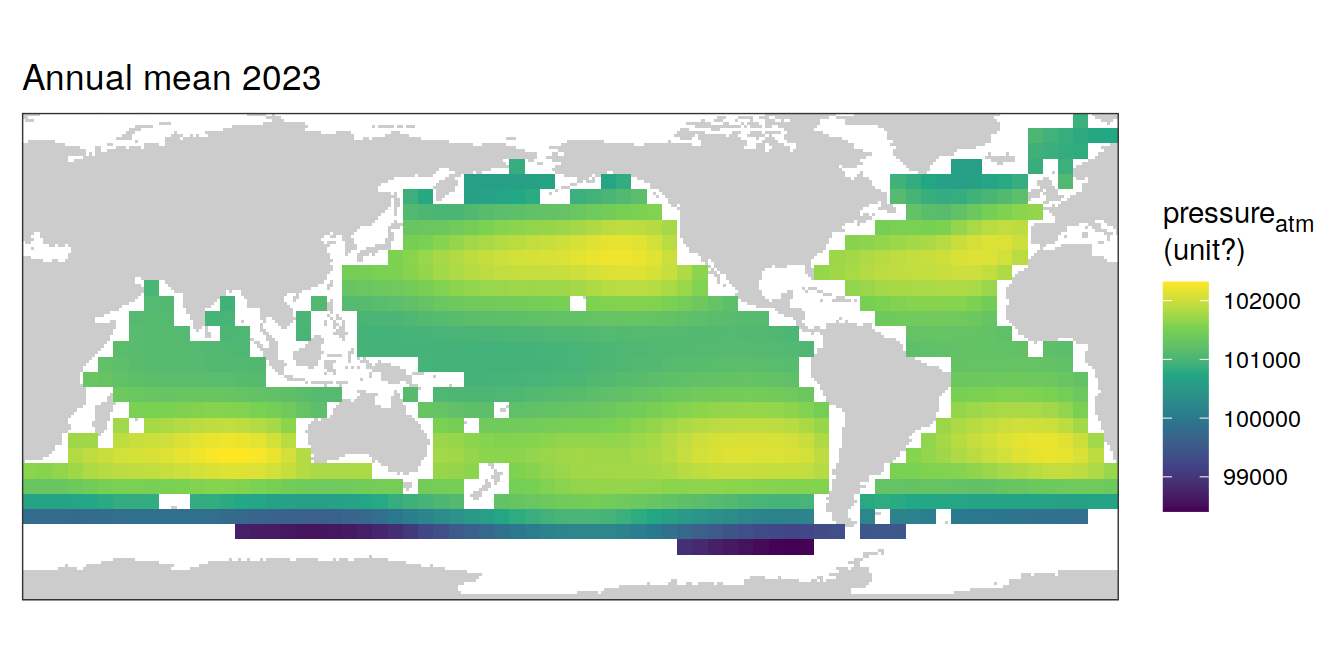
[[5]]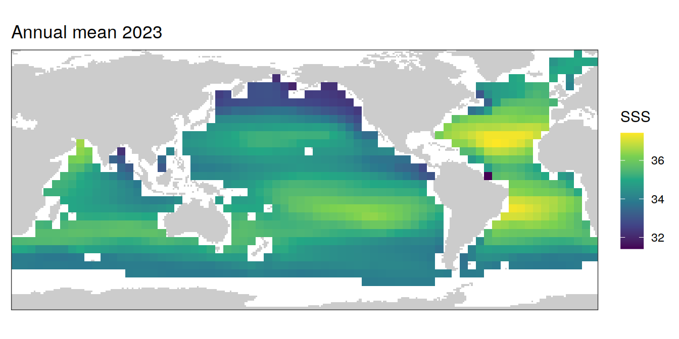
[[6]]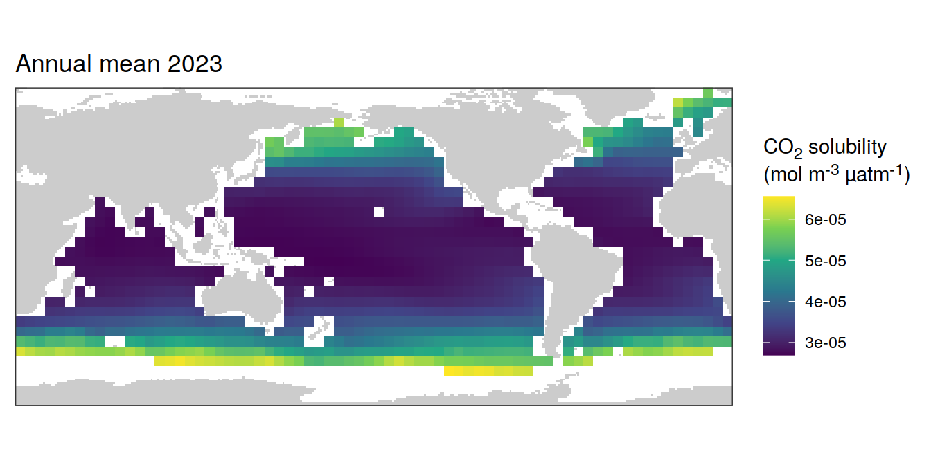
[[7]]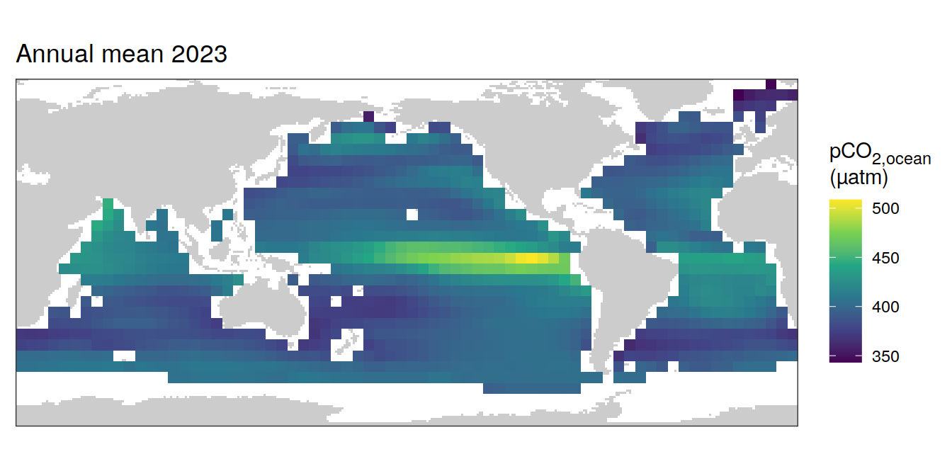
[[8]]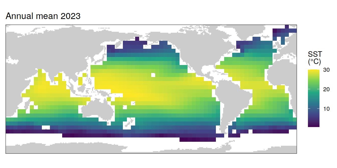
pco2_product_coarse_annual_regression %>%
  filter(year == 2023,
         name %in% name_divergent) %>%
  group_split(name) %>%
  # head(1) %>%
  map( ~ map +
         geom_tile(data = .x,
                   aes(lon, lat, fill = value)) +
         labs(title = "Annual mean 2023") +
         scale_fill_divergent(
           name = labels_breaks(.x %>% distinct(name))) +
         theme(legend.title = element_markdown())
  )
[[1]]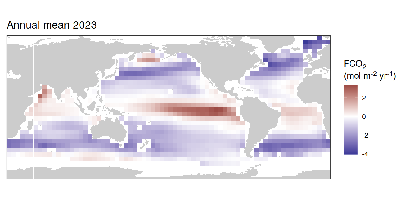
Trends
pco2_product_coarse_annual_regression %>%
  group_by(name) %>%
  filter(year %in% c(min(year), max(year))) %>%
  ungroup() %>%
  select(-c(value, resid)) %>%
  arrange(year) %>%
  group_by(lon, lat, name) %>%
  mutate(change = fit - lag(fit),
         period = paste(lag(year), year, sep = "-")) %>%
  ungroup() %>%
  filter(!is.na(change)) %>%
  group_split(name) %>%
  # head(1) %>%
  map(
    ~ map +
      geom_tile(data = .x,
                aes(lon, lat, fill = change)) +
      labs(title =  paste("Change: ",.x$period)) +
      scale_fill_divergent(name = labels_breaks(.x %>% distinct(name))) +
      theme(legend.title = element_markdown())
  )
[[1]]
[[2]]
[[3]]
[[4]]
[[5]]
[[6]]
[[7]]
[[8]]
| Version | Author | Date |
|---|---|---|
| 2d2fb75 | jens-daniel-mueller | 2024-03-20 |
[[9]]
| Version | Author | Date |
|---|---|---|
| 2d2fb75 | jens-daniel-mueller | 2024-03-20 |
[[10]]
| Version | Author | Date |
|---|---|---|
| 2d2fb75 | jens-daniel-mueller | 2024-03-20 |
2023 anomaly
pco2_product_coarse_annual_regression %>%
  filter(year == 2023) %>%
  group_split(name) %>%
  # head(1) %>%
  map( ~ map +
         geom_tile(data = .x,
                   aes(lon, lat, fill = resid)) +
         labs(title =  "2023 anomaly") +
         scale_fill_divergent(
           name = labels_breaks(.x %>% distinct(name))) +
         theme(legend.title = element_markdown())
  )
[[1]]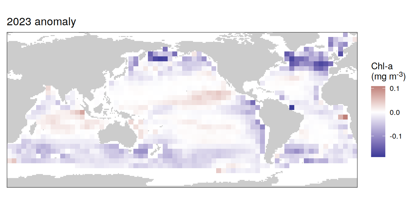
[[2]]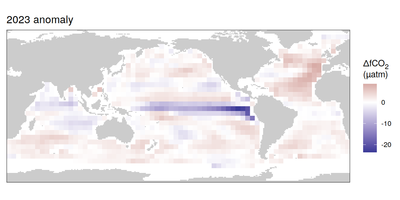
[[3]]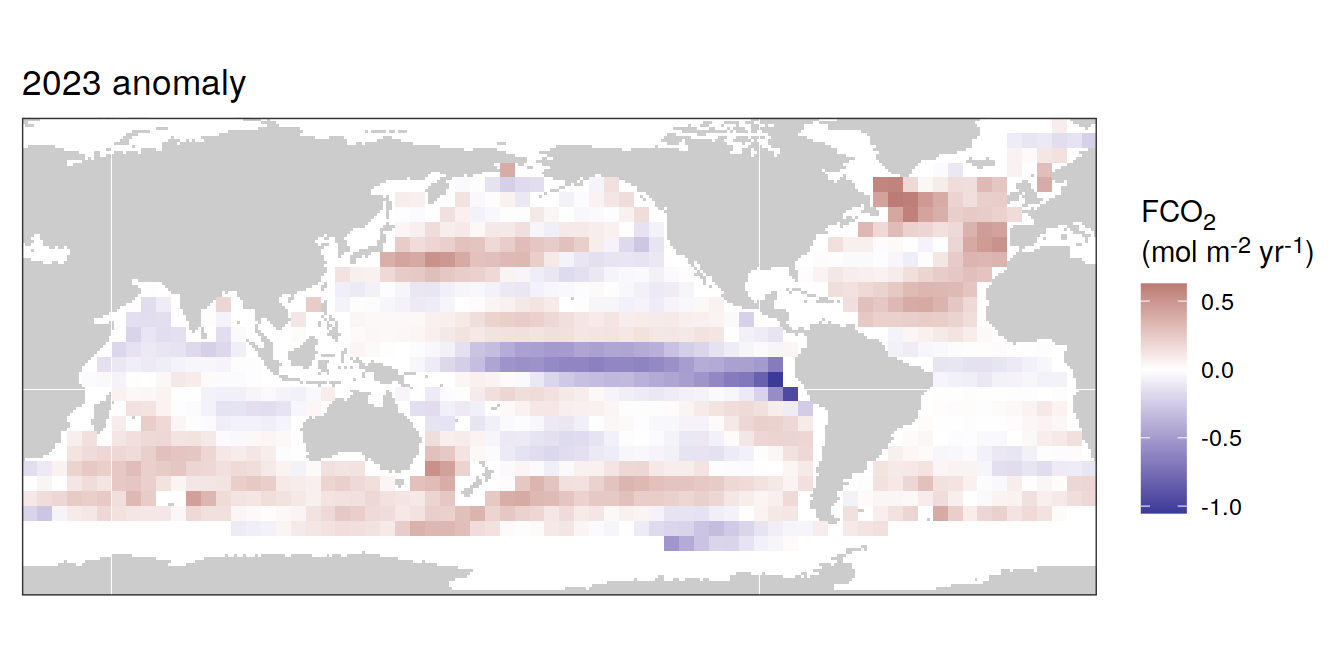
[[4]]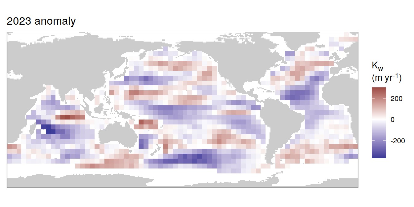
[[5]]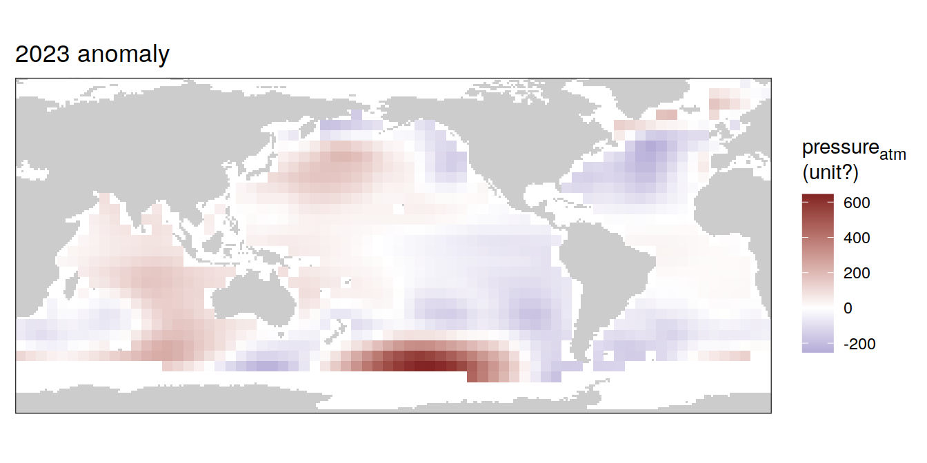
[[6]]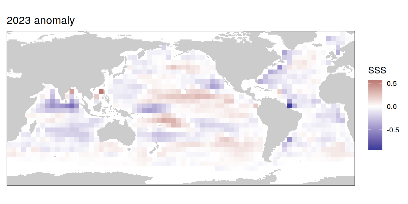
[[7]]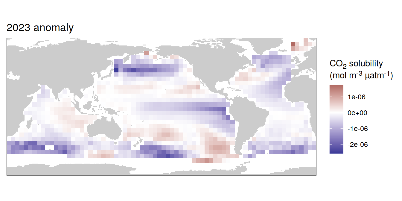
[[8]]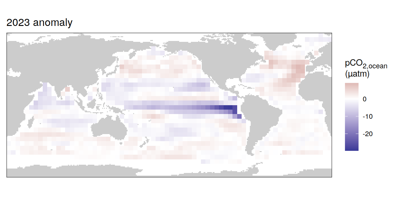
[[9]]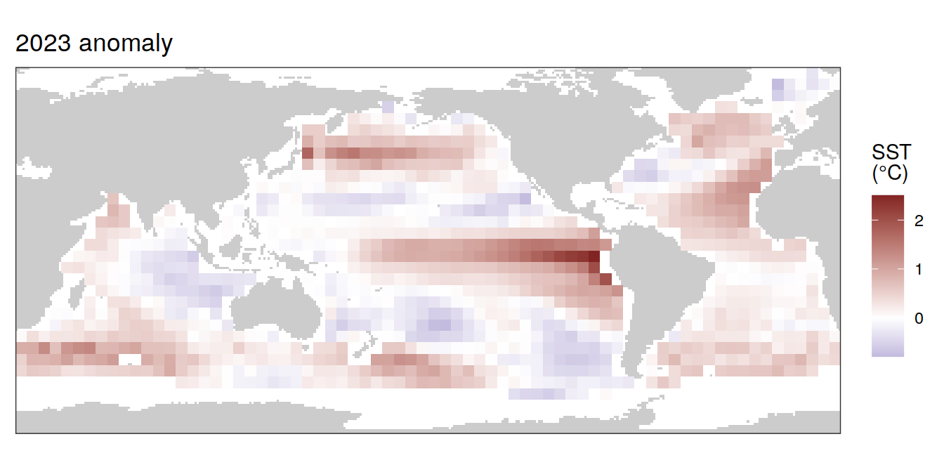
pco2_product_coarse_annual_regression %>%
  filter(year == 2023) %>%
  write_csv(paste0("../data/","OceanSODA","_anomaly_map_annual.csv"))
Monthly means
2023 absolute
pco2_product_coarse_monthly <-
  pco2_product_coarse %>%
  group_by(year, month, lon, lat) %>%
  summarise(across(where(is.numeric),
                   ~ mean(.))) %>%
  ungroup()

pco2_product_coarse_monthly <-
  pco2_product_coarse_monthly %>%
  pivot_longer(-c(year, month, lon, lat))

pco2_product_coarse_monthly_regression <-
  pco2_product_coarse_monthly %>%
  anomaly_determination(lon, lat, month)

pco2_product_coarse_monthly_regression <-
  pco2_product_coarse_monthly_regression %>%
  drop_na()


pco2_product_coarse_monthly_regression %>%
  filter(year == 2023,
         !(name %in% name_divergent)) %>%
  group_split(name) %>%
  # head(1) %>%
  map(
    ~ map +
      geom_tile(data = .x,
                aes(lon, lat, fill = value)) +
      labs(title = "Monthly means 2023") +
      scale_fill_viridis_c(name = labels_breaks(.x %>% distinct(name))) +
      theme(legend.title = element_markdown()) +
      facet_wrap( ~ month, ncol = 2)
  )
[[1]]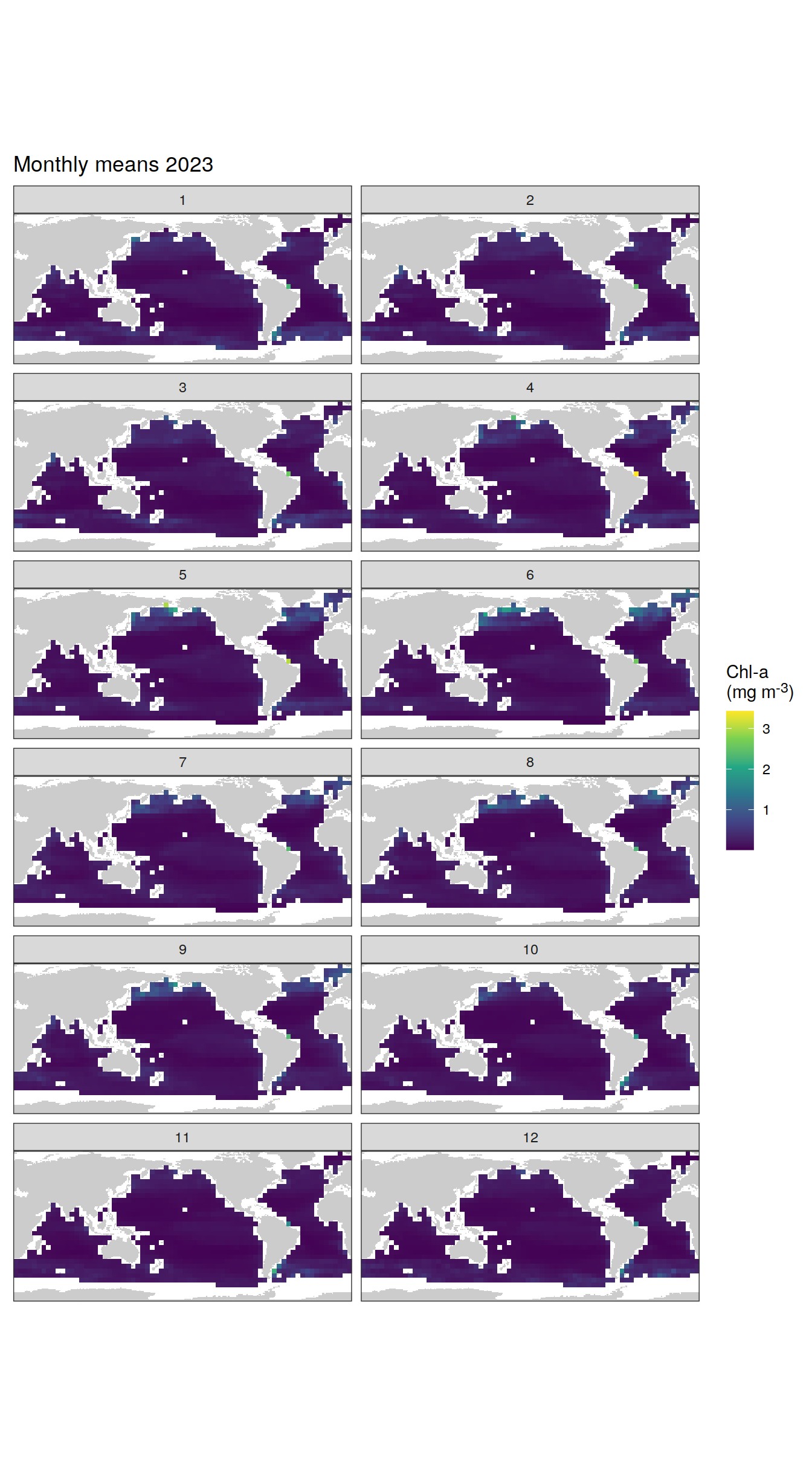
[[2]]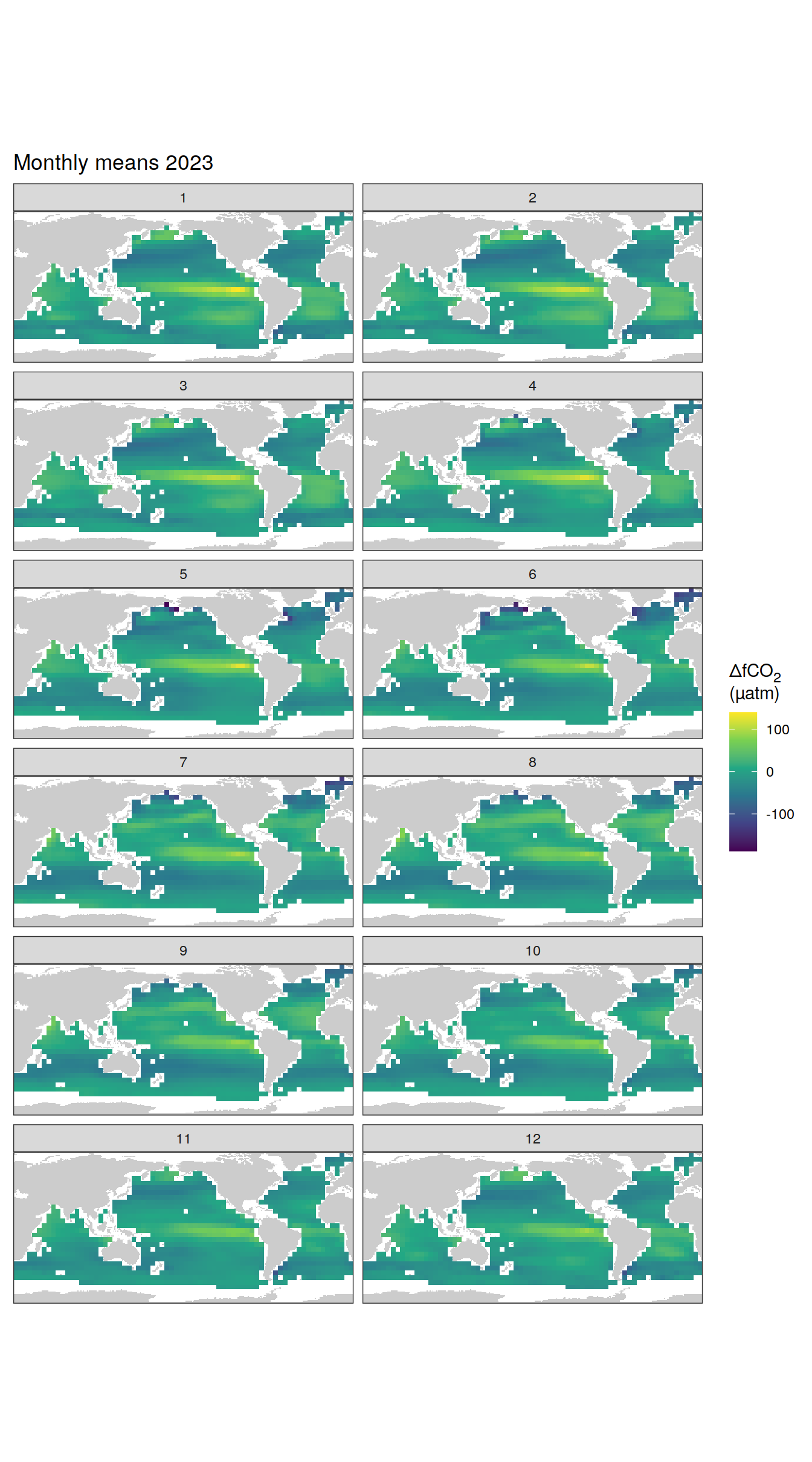
[[3]]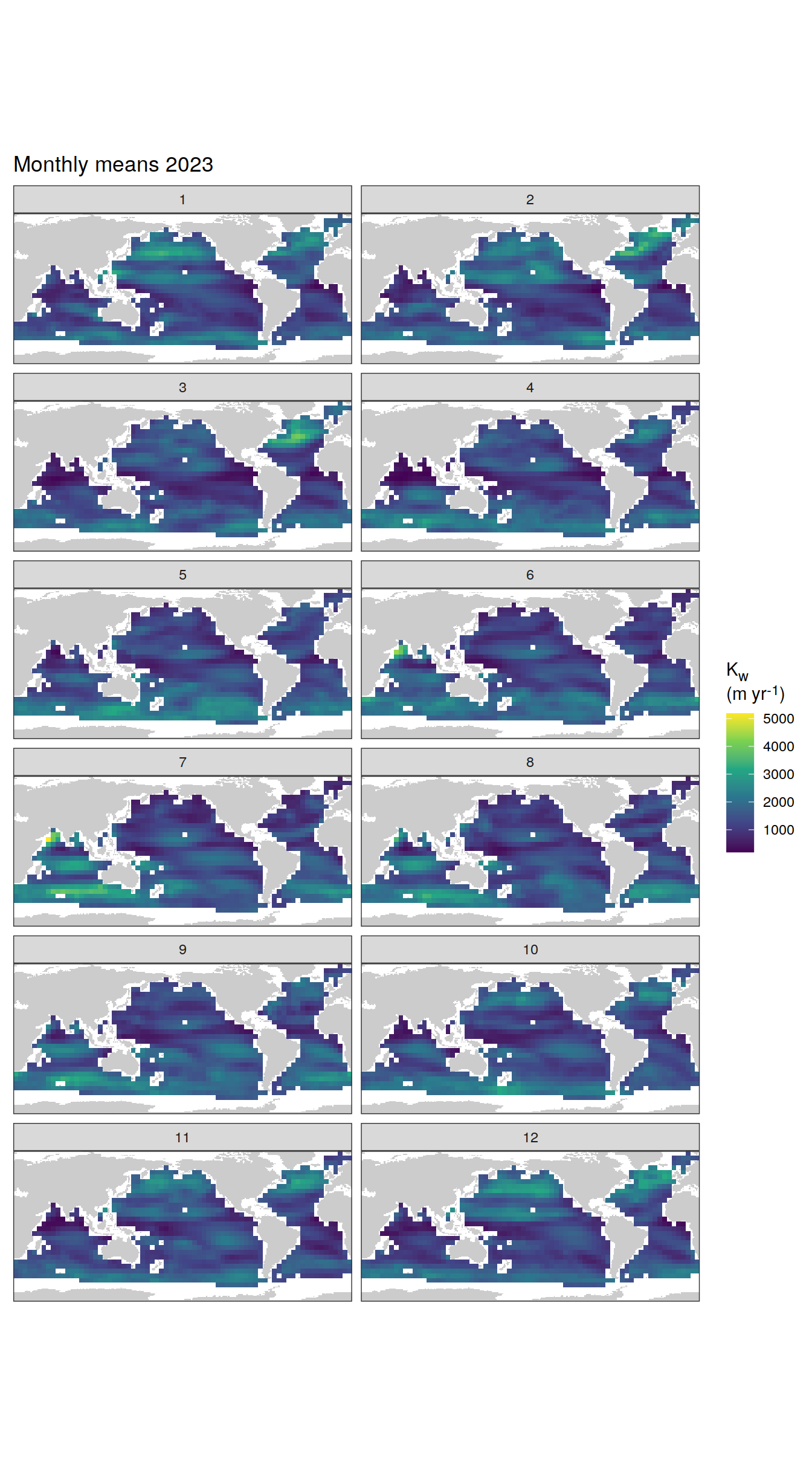
[[4]]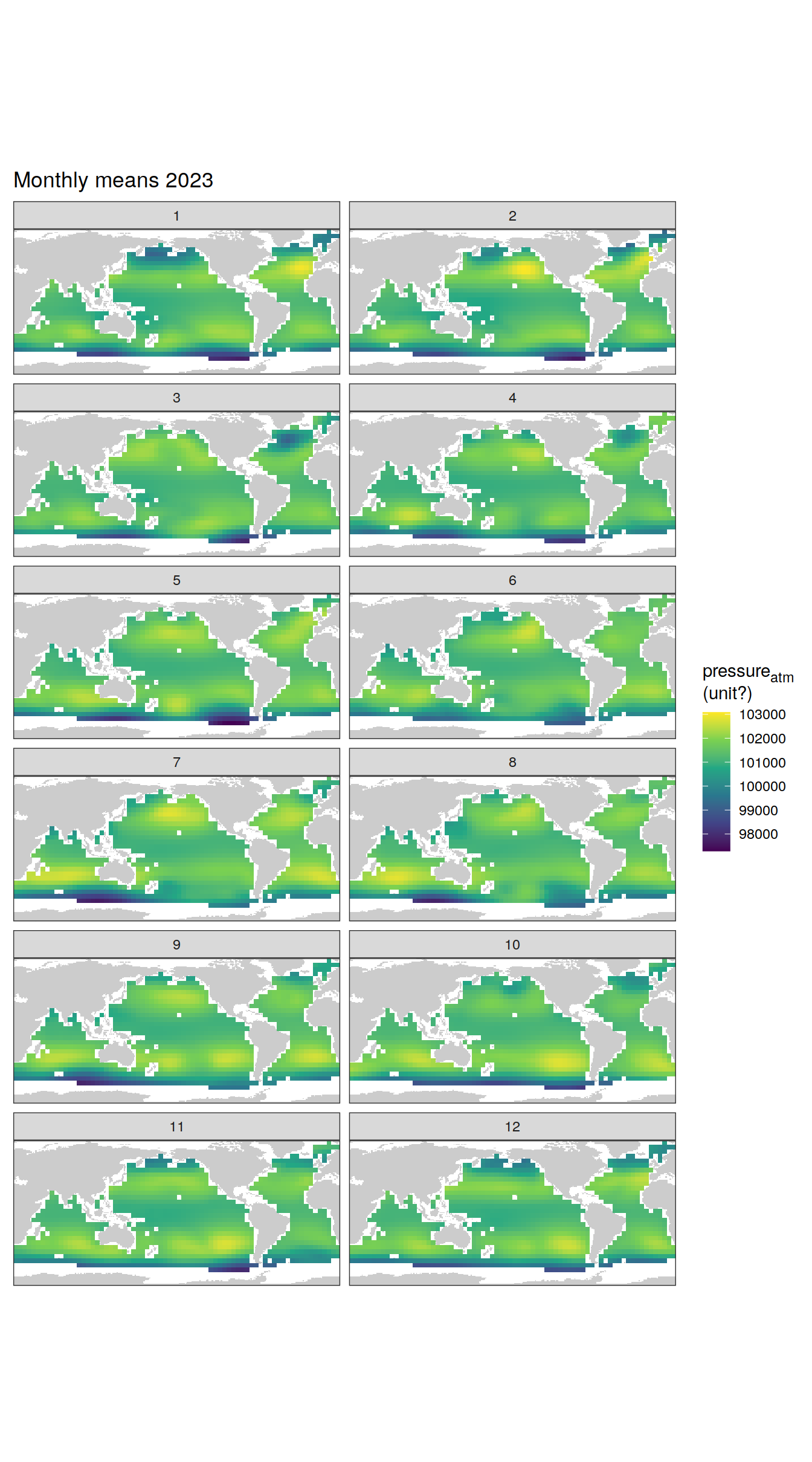
[[5]]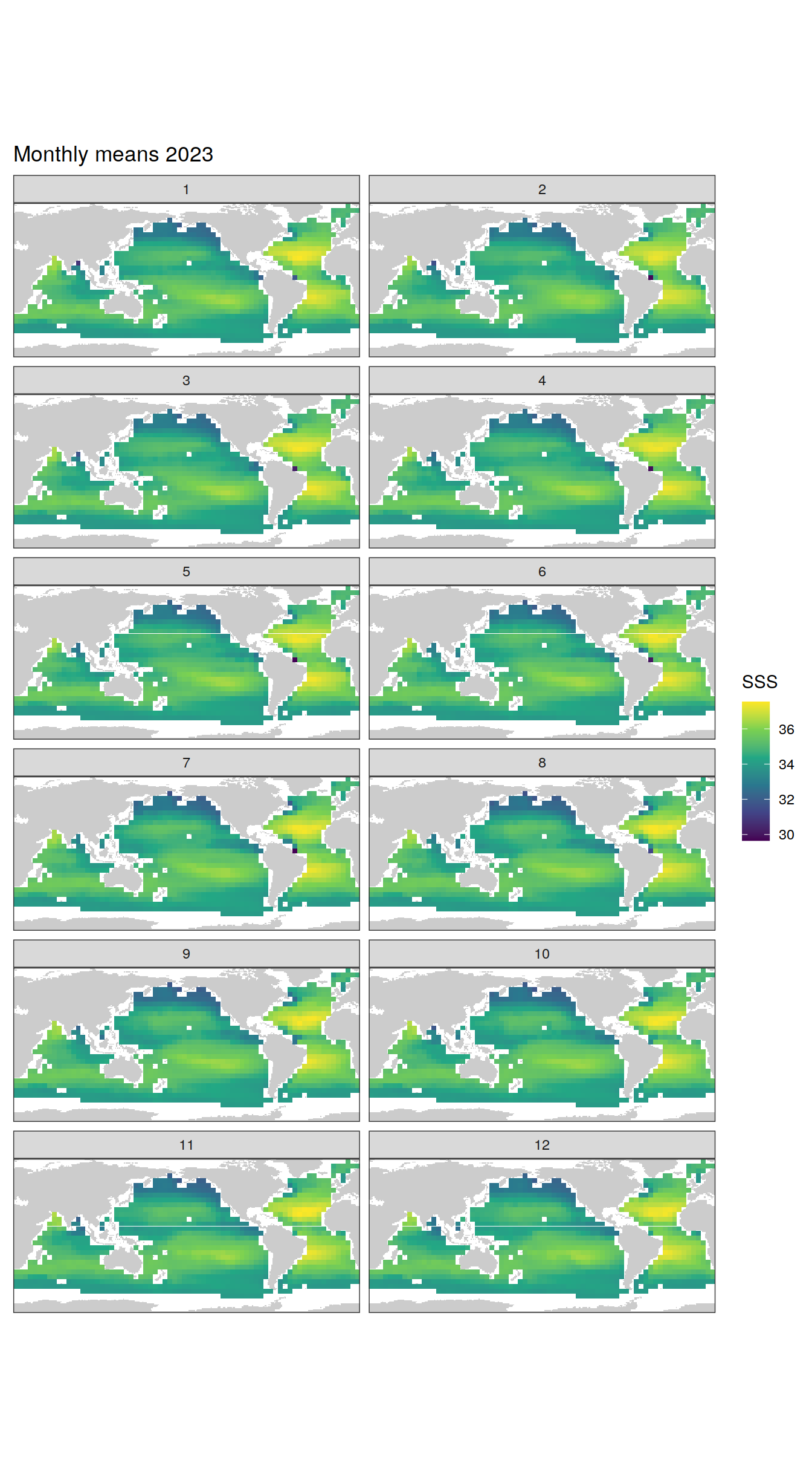
[[6]]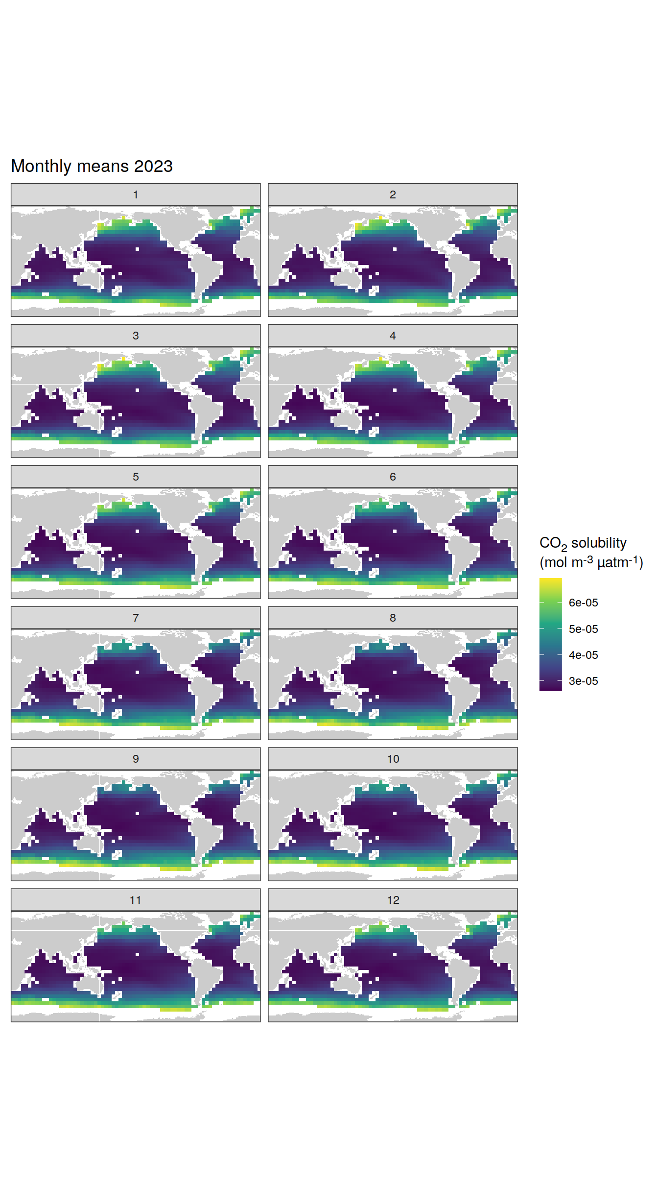
[[7]]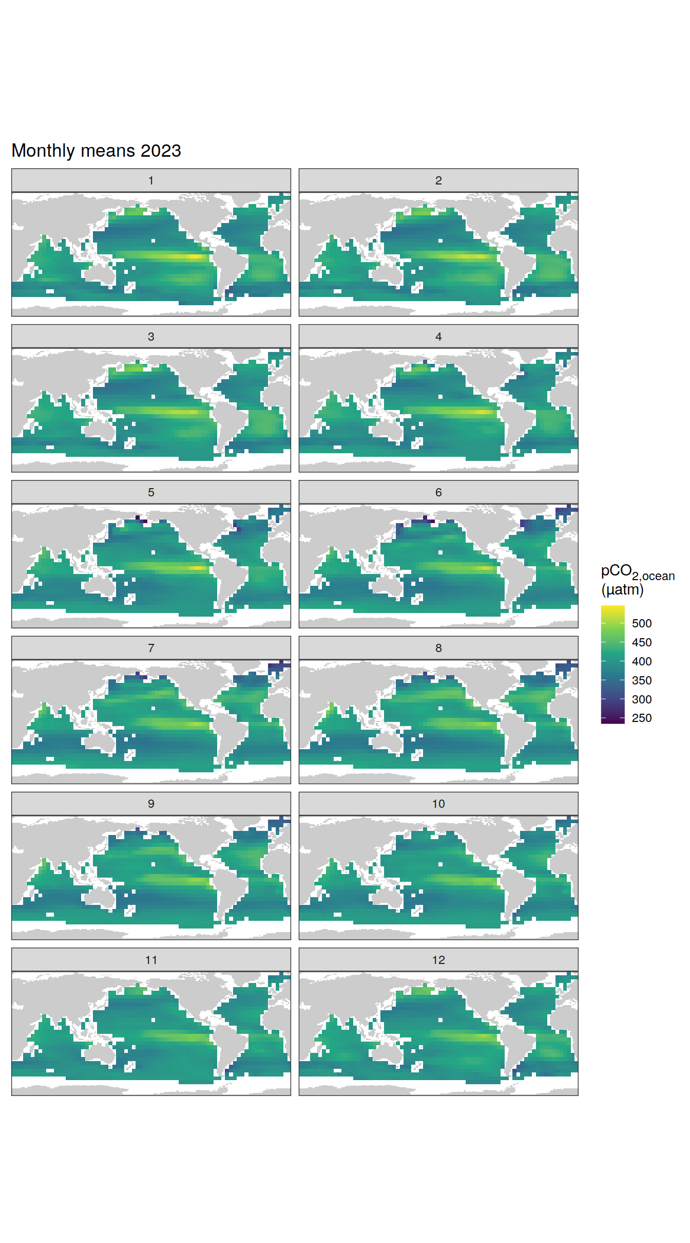
[[8]]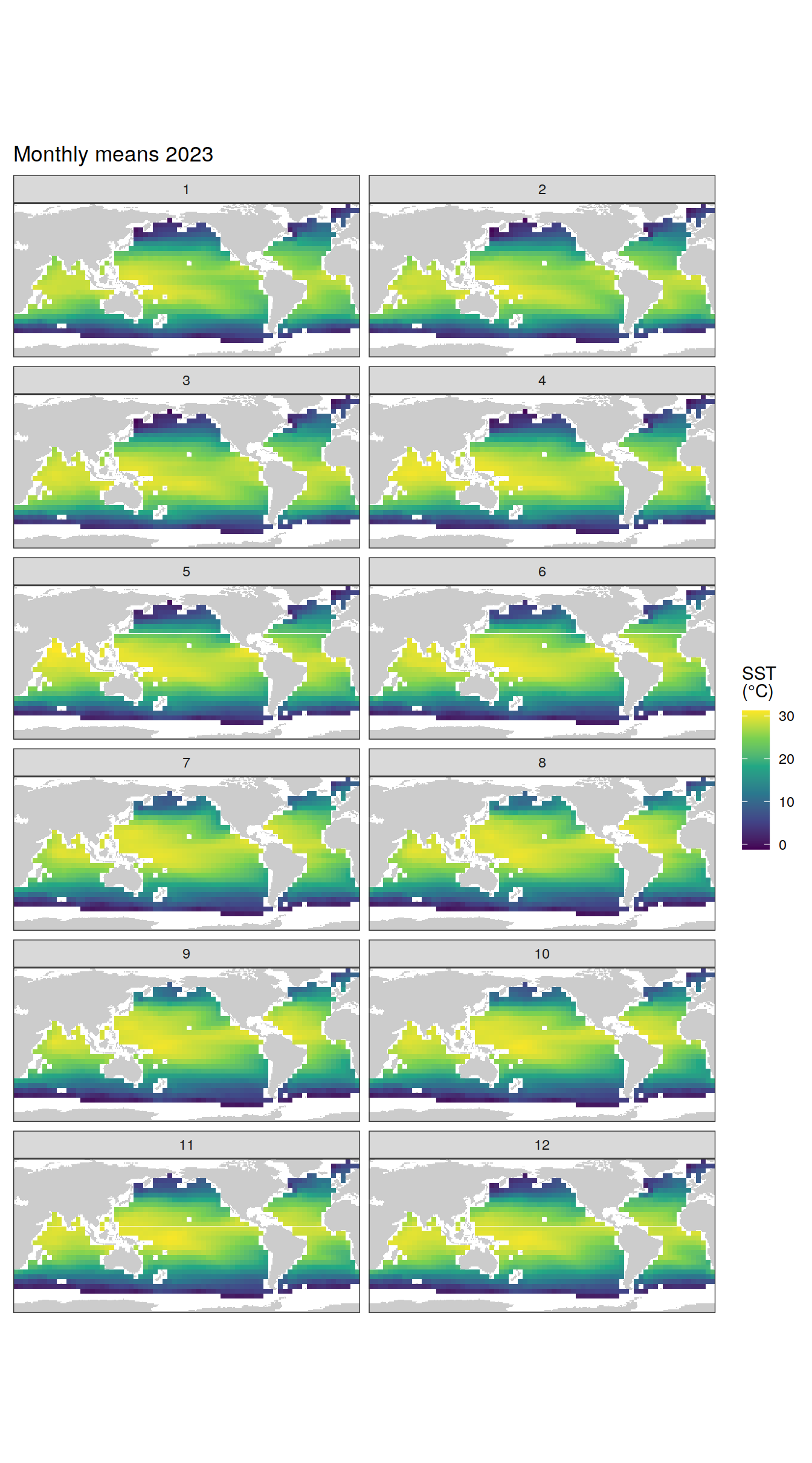
pco2_product_coarse_monthly_regression %>%
  filter(year == 2023,
         name %in% name_divergent) %>%
  group_split(name) %>%
  # head(1) %>%
  map(
    ~ map +
      geom_tile(data = .x,
                aes(lon, lat, fill = value)) +
      labs(title = "Monthly means 2023") +
      scale_fill_divergent(name = labels_breaks(.x %>% distinct(name))) +
      theme(legend.title = element_markdown()) +
      facet_wrap( ~ month, ncol = 2)
  )
[[1]]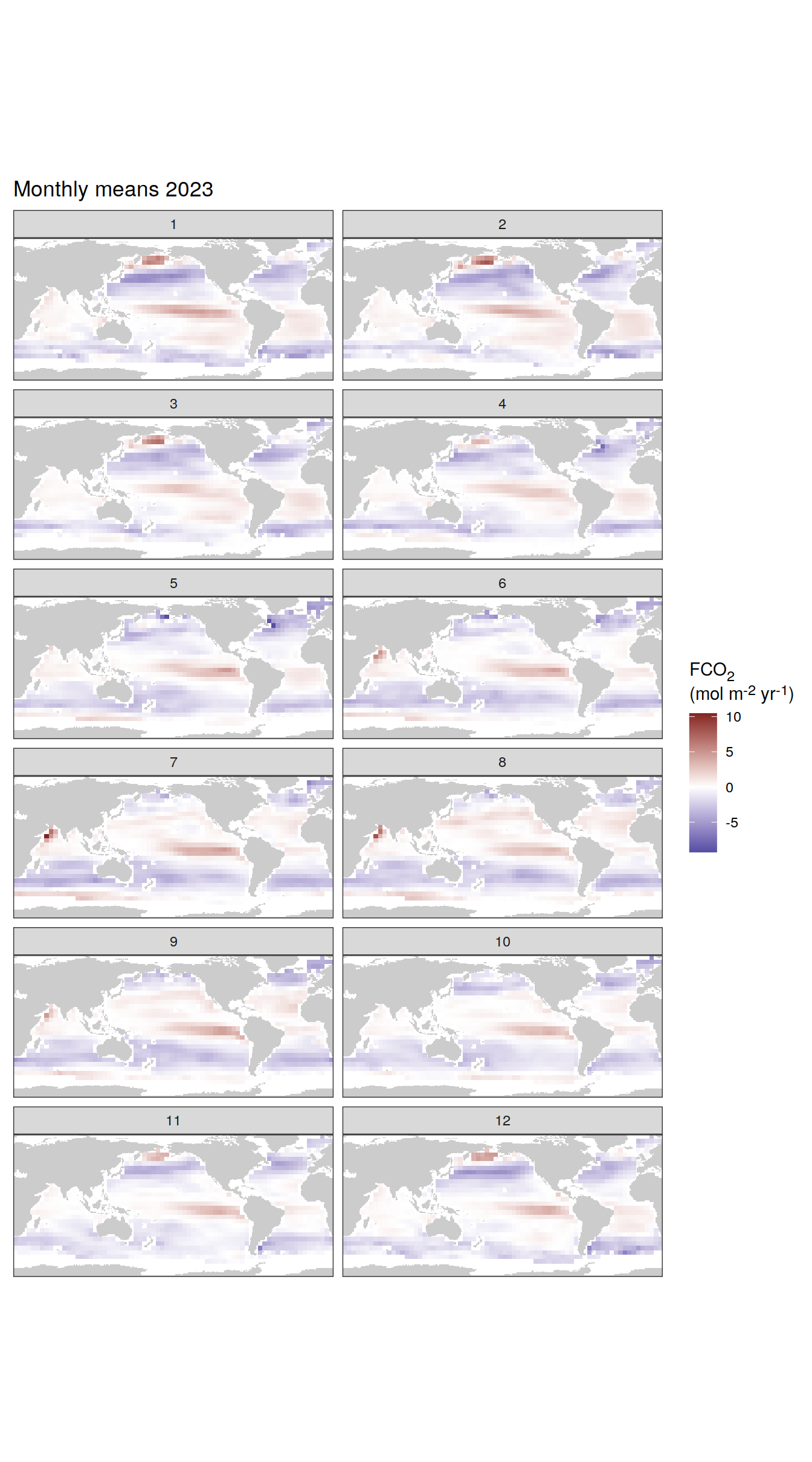
Trends
pco2_product_coarse_monthly_regression %>%
  group_by(name) %>%
  filter(year %in% c(min(year), max(year))) %>%
  ungroup() %>%
  select(-c(value, resid)) %>%
  arrange(year) %>%
  group_by(lon, lat, name, month) %>%
  mutate(change = fit - lag(fit),
         period = paste(lag(year), year, sep = "-")) %>%
  ungroup() %>%
  filter(!is.na(change)) %>%
  group_split(name) %>%
  # head(1) %>%
  map(
    ~ map +
      geom_tile(data = .x,
                aes(lon, lat, fill = change)) +
      labs(title =  paste("Change: ", .x$period)) +
      scale_fill_divergent(name = labels_breaks(.x %>% distinct(name))) +
      theme(legend.title = element_markdown()) +
      facet_wrap(~ month, ncol = 2)
  )
[[1]]
[[2]]
[[3]]
[[4]]
[[5]]
[[6]]
[[7]]
[[8]]
| Version | Author | Date |
|---|---|---|
| 2d2fb75 | jens-daniel-mueller | 2024-03-20 |
[[9]]
| Version | Author | Date |
|---|---|---|
| 2d2fb75 | jens-daniel-mueller | 2024-03-20 |
[[10]]
| Version | Author | Date |
|---|---|---|
| 2d2fb75 | jens-daniel-mueller | 2024-03-20 |
2023 anomaly
pco2_product_coarse_monthly_regression %>%
  filter(year == 2023) %>%
  group_split(name) %>%
  # head(1) %>%
  map(
    ~ map +
      geom_tile(data = .x,
                aes(lon, lat, fill = resid)) +
      labs(title = "2023 anomaly") +
      scale_fill_divergent(name = labels_breaks(.x %>% distinct(name))) +
      theme(legend.title = element_markdown()) +
      facet_wrap( ~ month, ncol = 2)
  )
[[1]]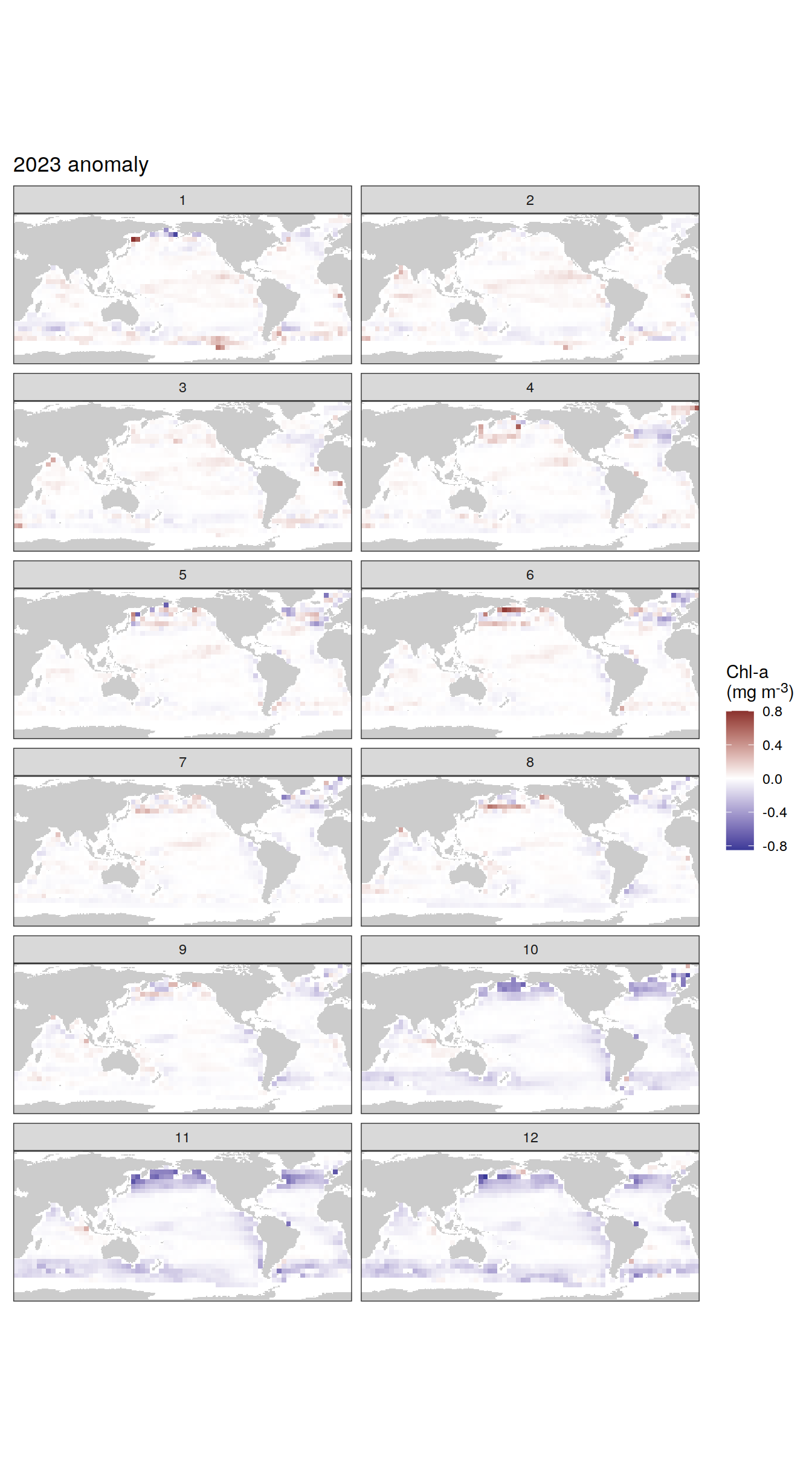
[[2]]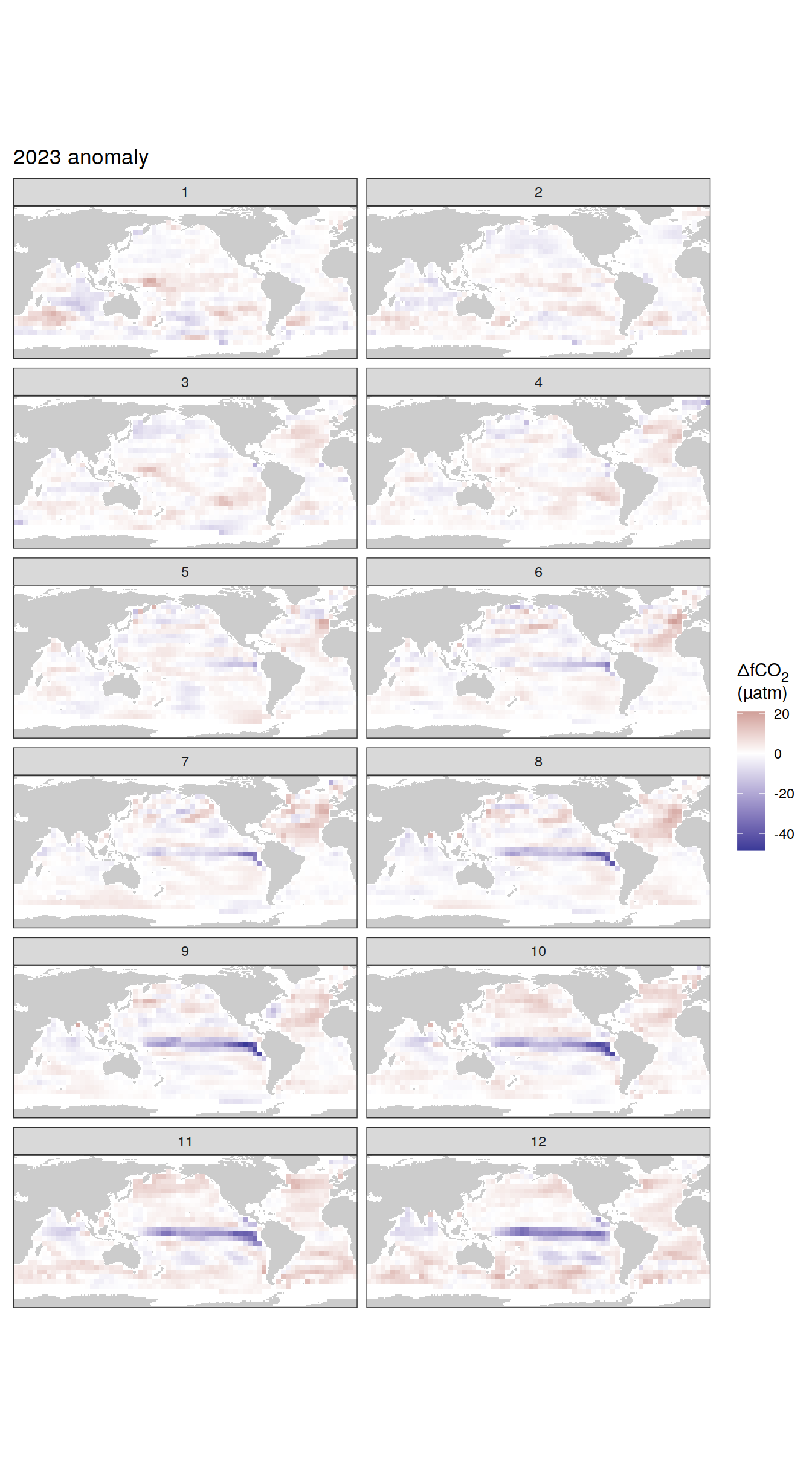
[[3]]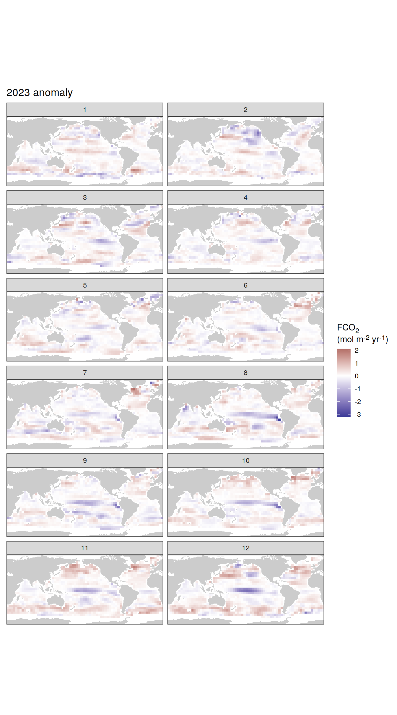
[[4]]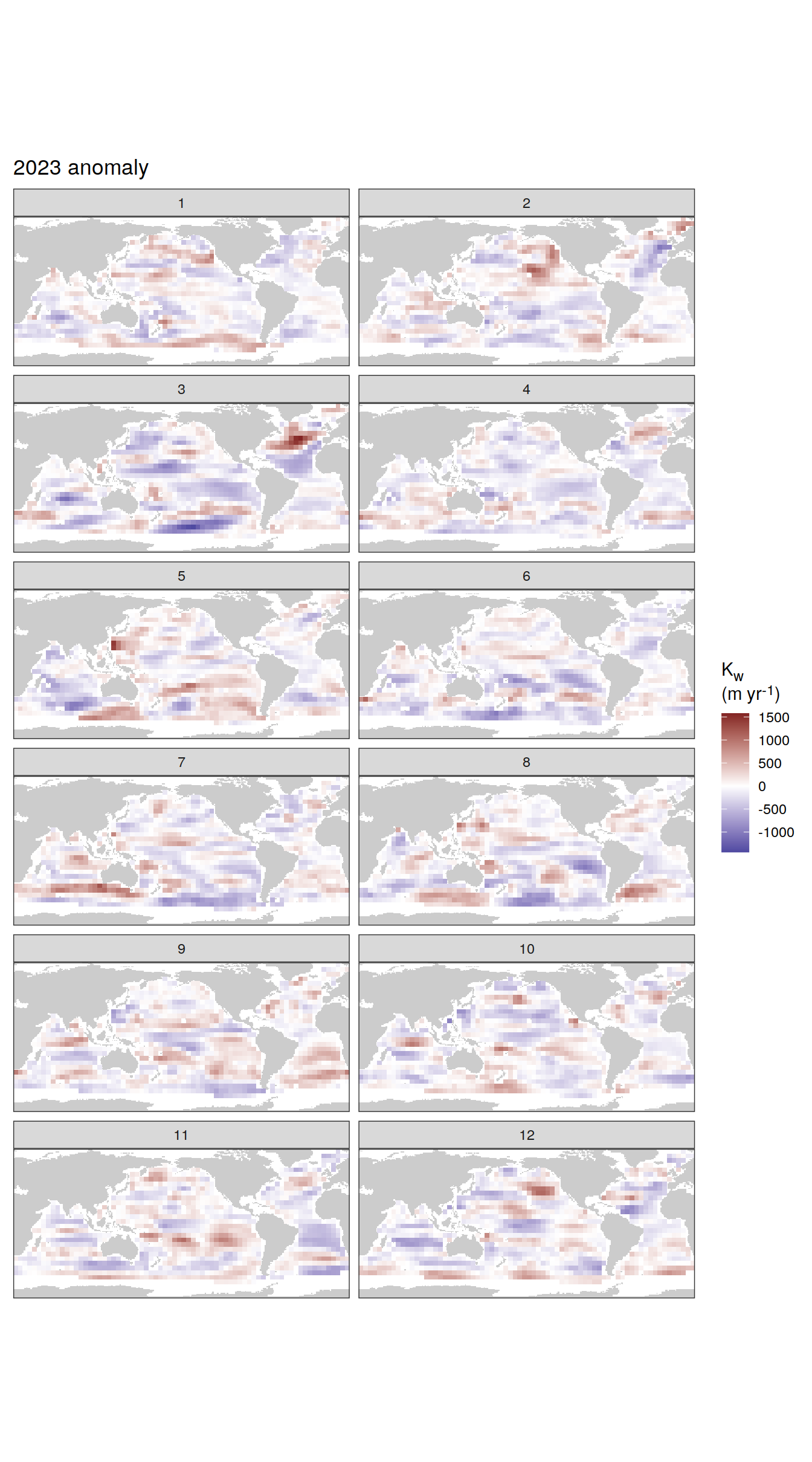
[[5]]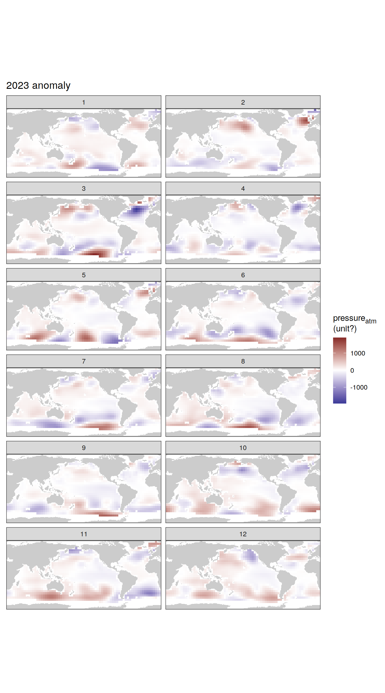
[[6]]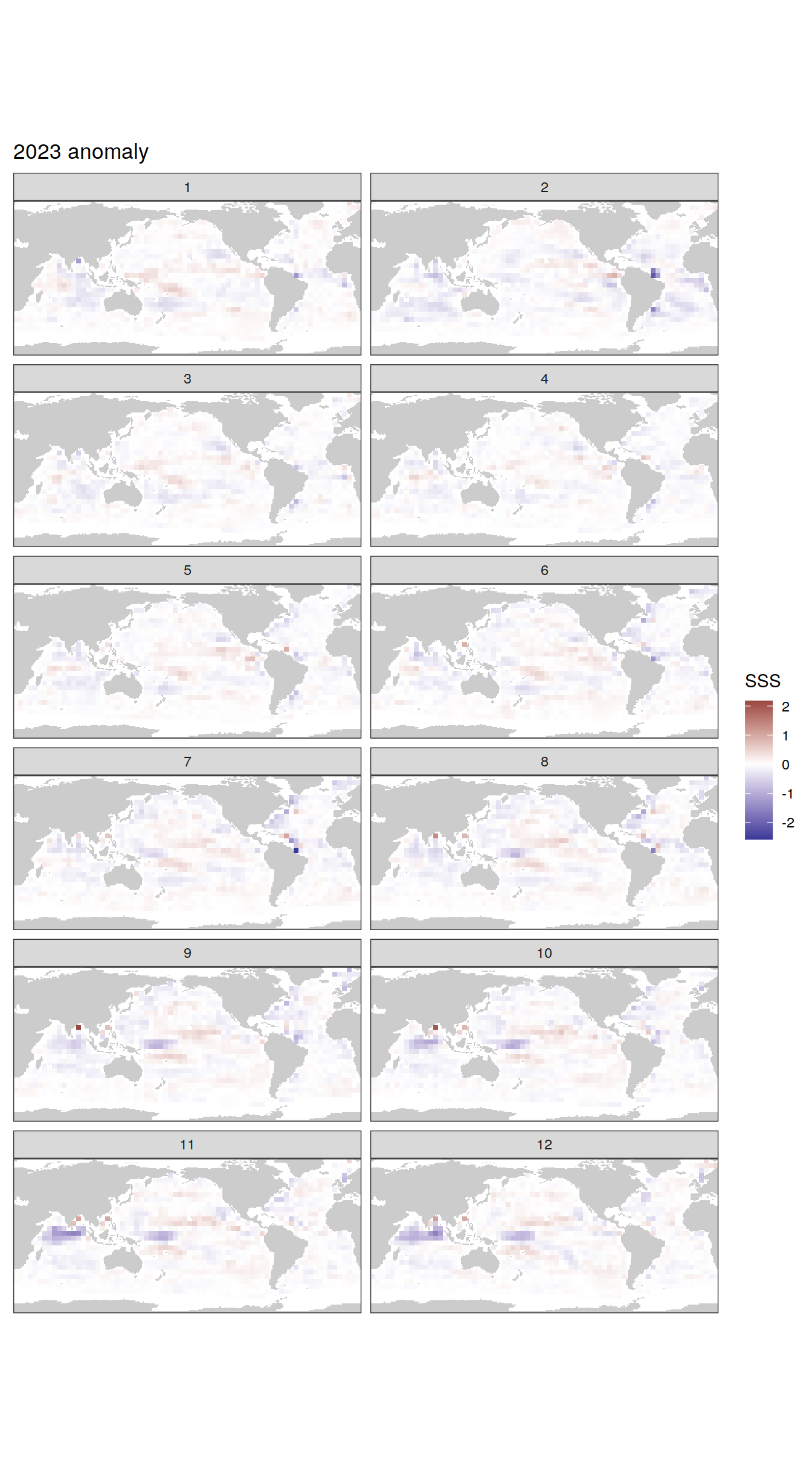
[[7]]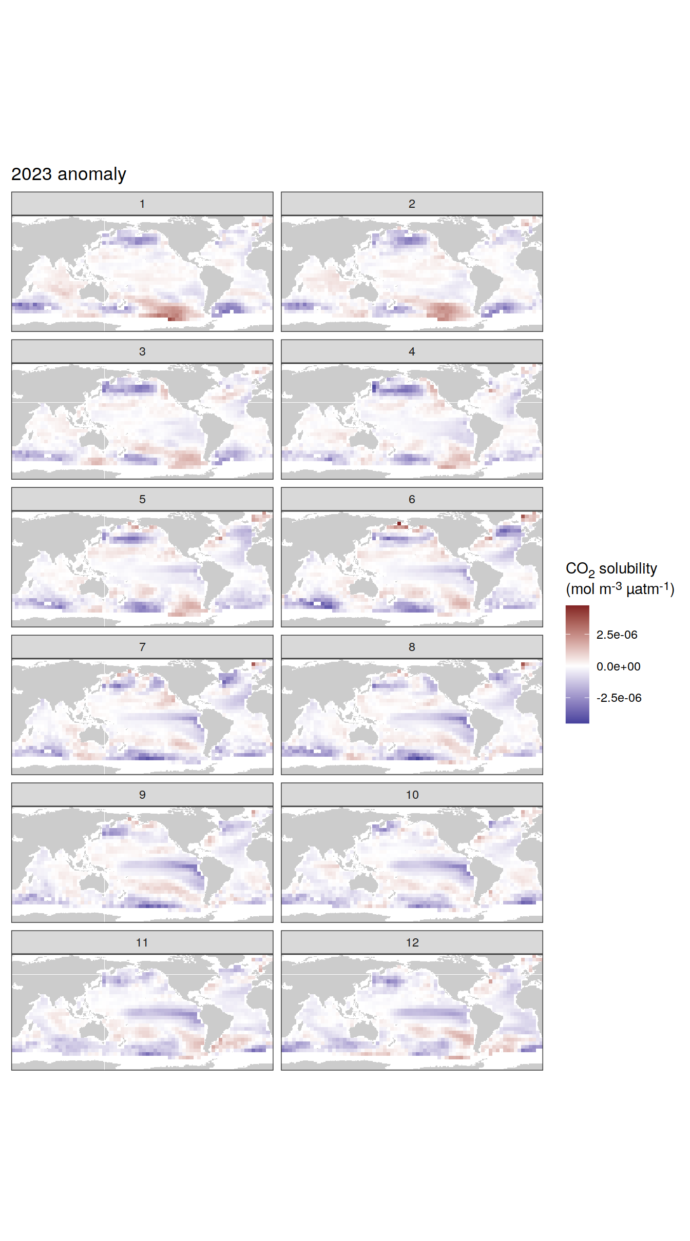
[[8]]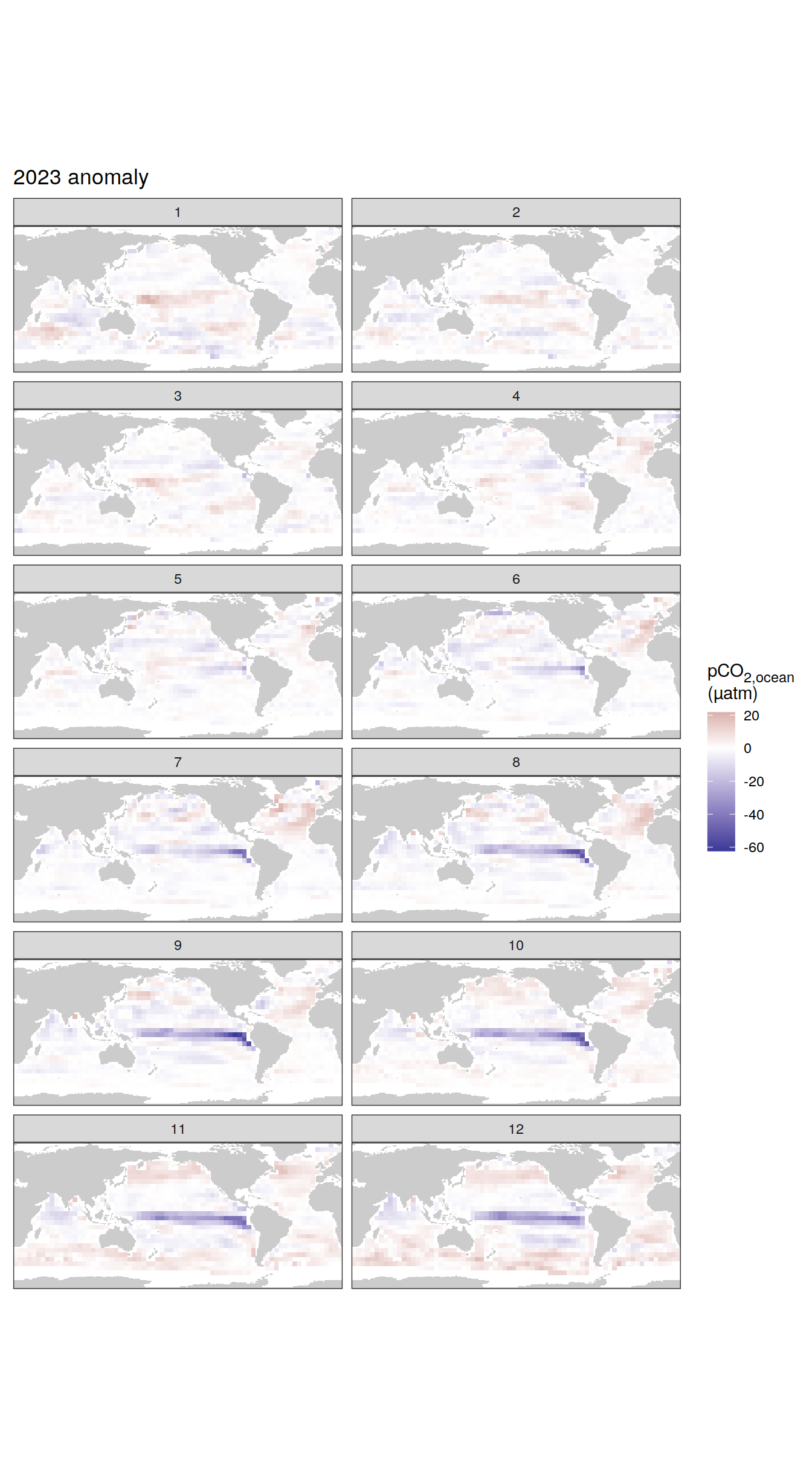
[[9]]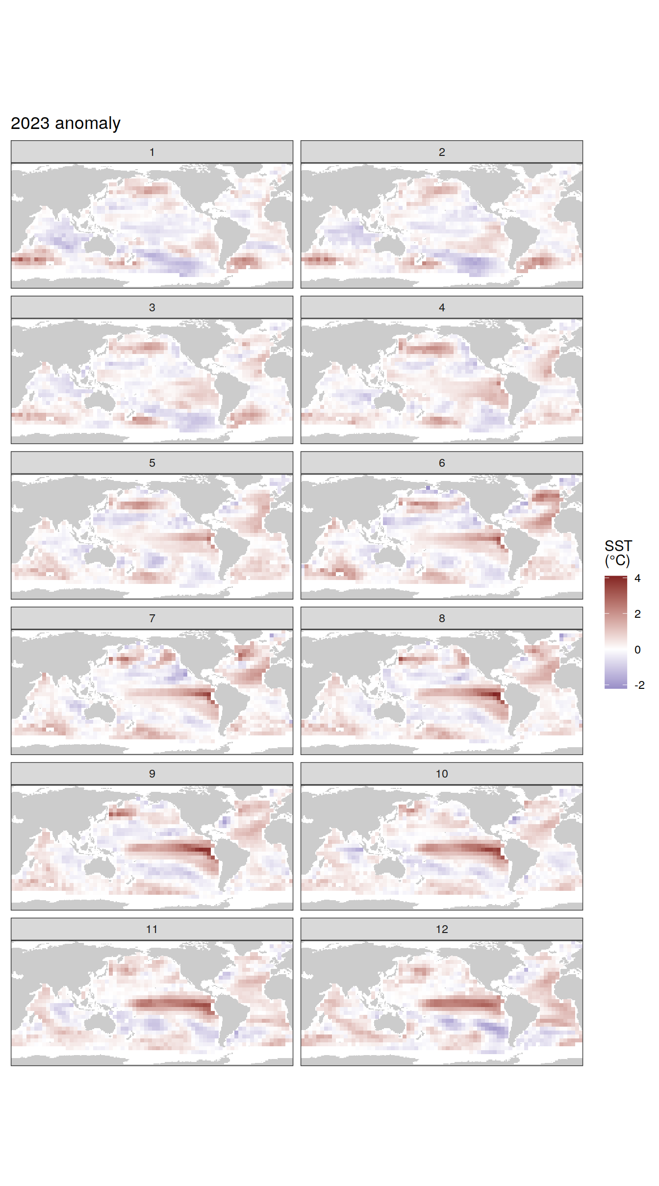
pco2_product_coarse_monthly_regression %>%
  filter(year == 2023) %>%
  write_csv(paste0("../data/","OceanSODA","_anomaly_map_monthly.csv"))
Hovmoeller plots
The following Hovmoeller plots show the value of each variable as provided through the pCO2 product, as well as the anomalies from the prediction of a linear/quadratic fit to the data from 1990 to 2022.
Hovmoeller plots are first presented as annual means, and than as monthly means. Note that the predictions for the monthly Hovmoeller plots are done individually for each month, such the mean seasonal anomaly from the annual mean is removed.
Annual means
Absolute
pco2_product_hovmoeller_monthly_annual <-
  pco2_product %>%
  select(-c(lon, time, month, biome)) %>%
  group_by(year, lat) %>%
  summarise(across(-c(fgco2, area),
                   ~ weighted.mean(., area, na.rm = TRUE)),
            across(fgco2,
                   ~ sum(. * area, na.rm = TRUE) * 12.01 * 1e-15)) %>%
  ungroup() %>%
  rename(fgco2_hov = fgco2) %>%
  filter(fgco2_hov != 0)

pco2_product_hovmoeller_monthly_annual <-
  pco2_product_hovmoeller_monthly_annual %>%
  pivot_longer(-c(year, lat)) %>%
  drop_na()

pco2_product_hovmoeller_monthly_annual %>%
  filter(!(name %in% name_divergent)) %>%
  group_split(name) %>%
  # head(1) %>%
  map(
    ~ ggplot(data = .x,
             aes(year, lat, fill = value)) +
      geom_raster() +
      scale_fill_viridis_c(name = labels_breaks(.x %>% distinct(name))) +
      theme(legend.title = element_markdown()) +
      coord_cartesian(expand = 0) +
      labs(title = "Annual means",
           y = "Latitude") +
      theme(axis.title.x = element_blank())
  )
[[1]]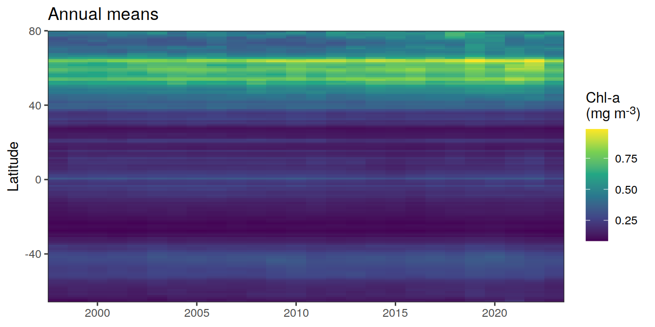
[[2]]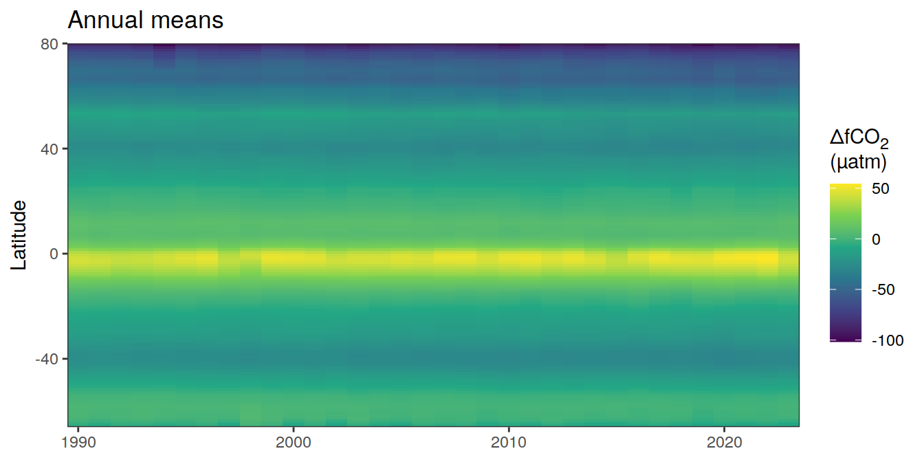
[[3]]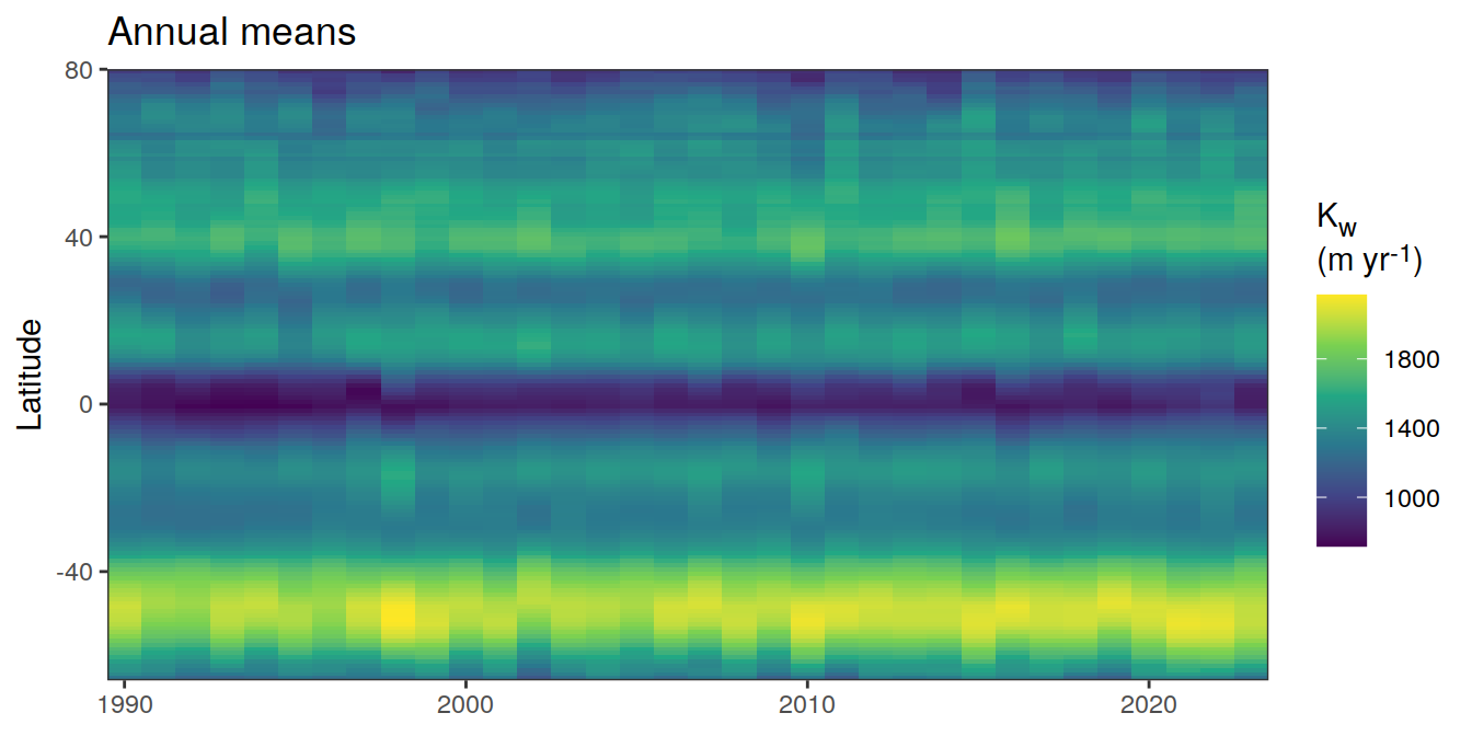
[[4]]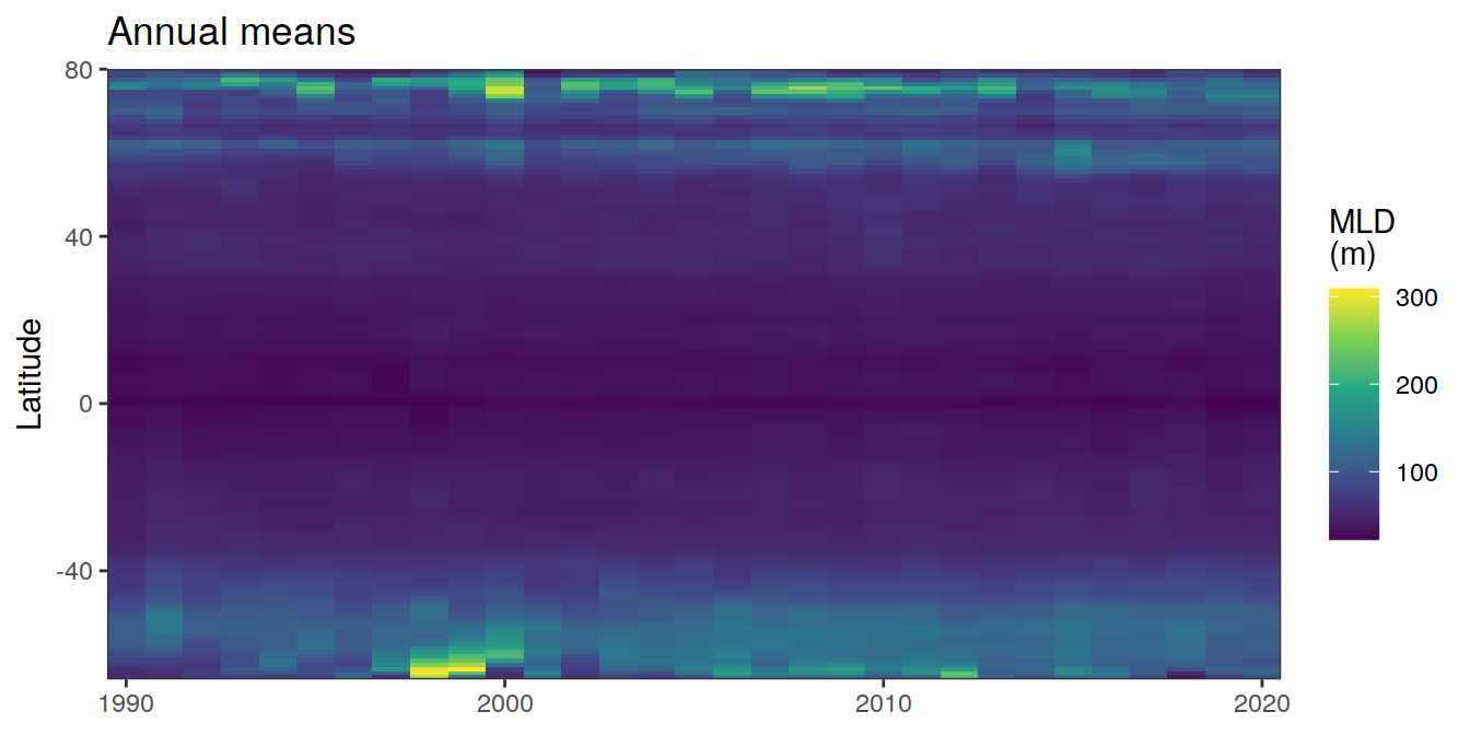
[[5]]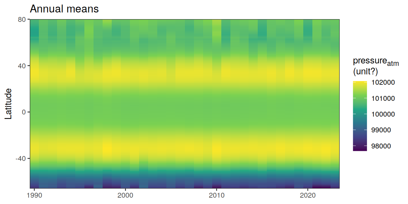
[[6]]
[[7]]
[[8]]
[[9]]
pco2_product_hovmoeller_monthly_annual %>%
  filter(name %in% name_divergent) %>%
  group_split(name) %>%
  # head(1) %>%
  map(
    ~ ggplot(data = .x,
             aes(year, lat, fill = value)) +
      geom_raster() +
      scale_fill_divergent(name = labels_breaks(.x %>% distinct(name))) +
      theme(legend.title = element_markdown()) +
      coord_cartesian(expand = 0) +
      labs(title = "Annual means",
           y = "Latitude") +
      theme(axis.title.x = element_blank())
  )
[[1]]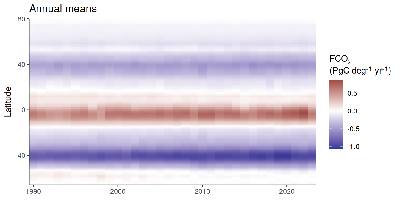
Anomalies
pco2_product_hovmoeller_monthly_annual_regression <-
  pco2_product_hovmoeller_monthly_annual %>%
  anomaly_determination(lat) %>%
  filter(!is.na(resid))


pco2_product_hovmoeller_monthly_annual_regression %>%
  # filter(name == "mld") %>%
  group_split(name) %>%
  # head(1) %>%
  map(
    ~ ggplot(data = .x,
             aes(year, lat, fill = resid)) +
      geom_raster() +
      scale_fill_divergent(name = labels_breaks(.x %>% distinct(name))) +
      theme(legend.title = element_markdown()) +
      coord_cartesian(expand = 0) +
      labs(title = "Annual mean anomalies",
           y = "Latitude") +
      theme(axis.title.x = element_blank())
  )
[[1]]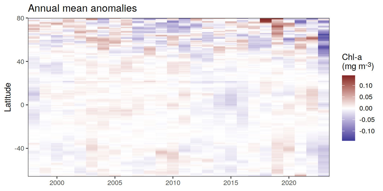
[[2]]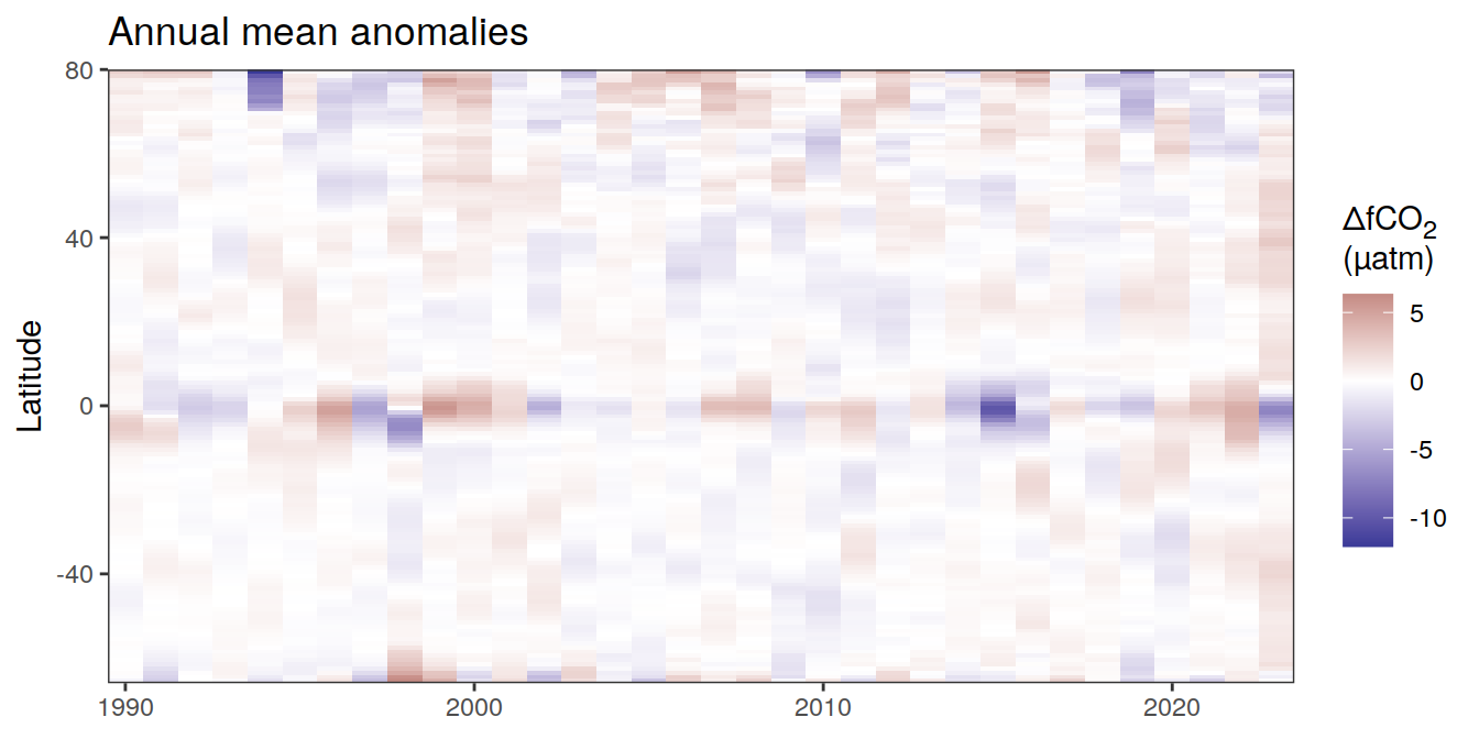
[[3]]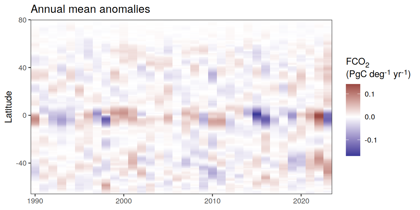
[[4]]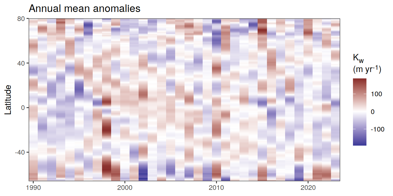
[[5]]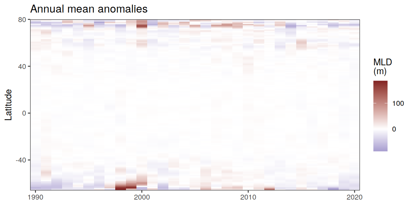
[[6]]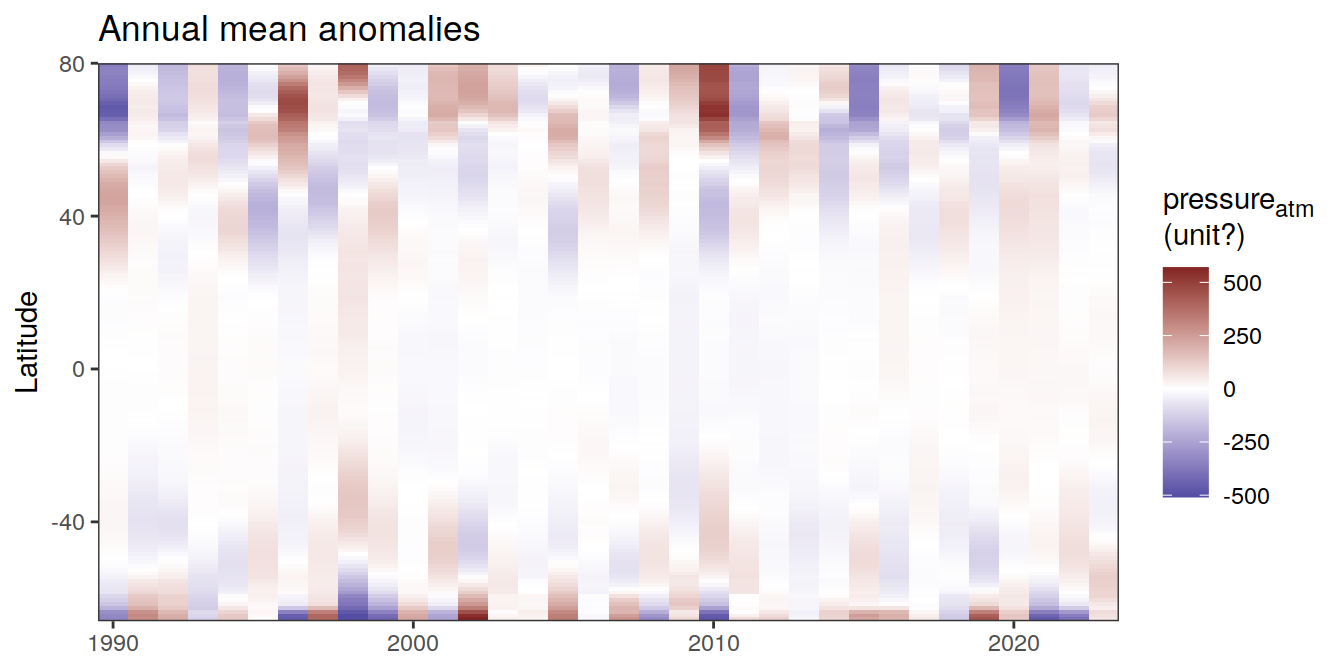
[[7]]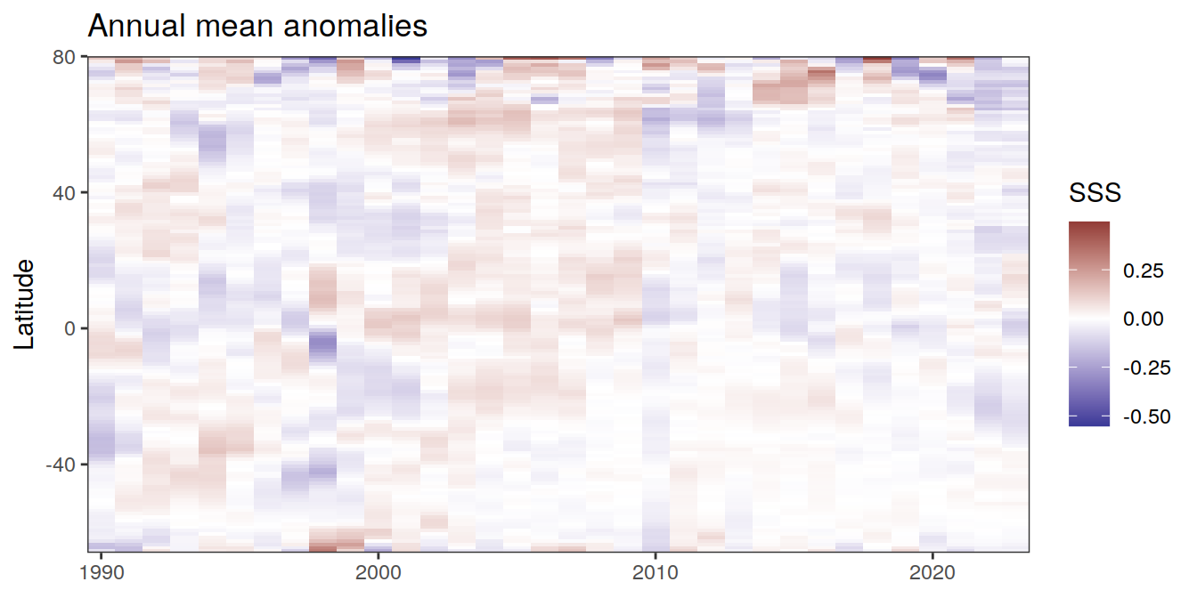
[[8]]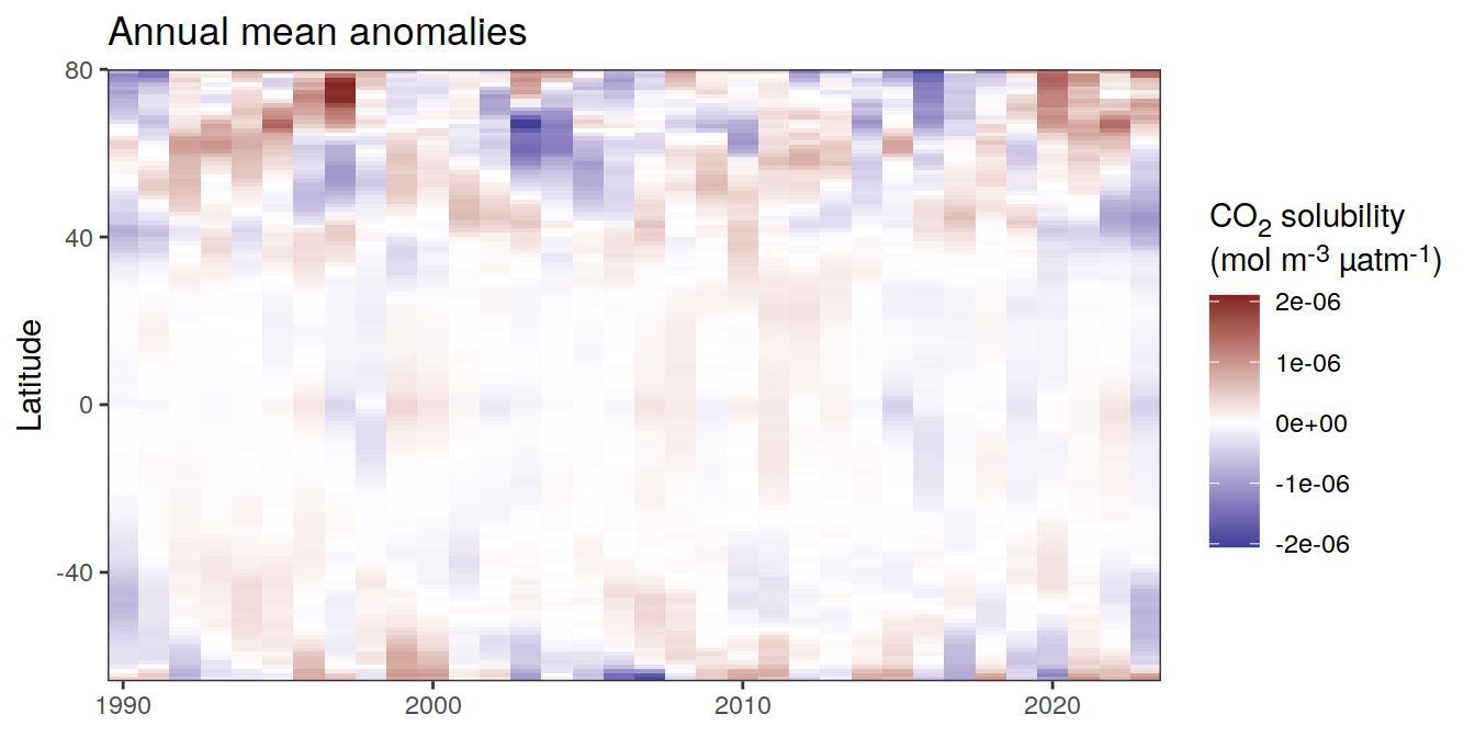
[[9]]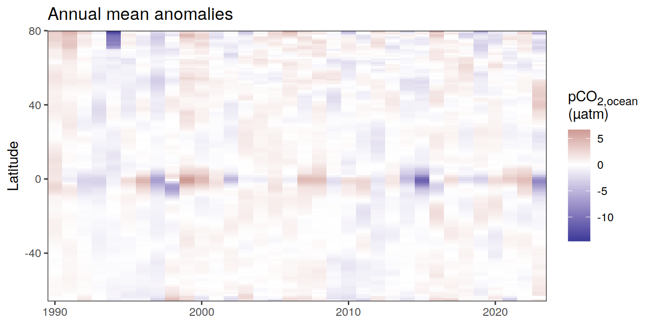
[[10]]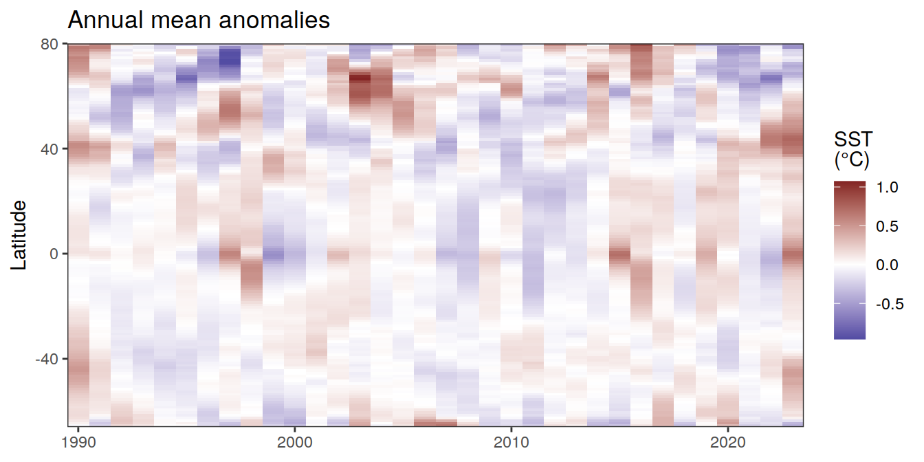
Monthly means
Absolute
pco2_product_hovmoeller_monthly <-
  pco2_product %>%
  select(-c(lon, time, biome)) %>%
  group_by(year, month, lat) %>%
  summarise(across(-c(fgco2, area),
                   ~ weighted.mean(., area, na.rm = TRUE)),
            across(fgco2,
                   ~ sum(. * area, na.rm = TRUE) * 12.01 * 1e-15)) %>%
  ungroup() %>%
  rename(fgco2_hov = fgco2) %>%
  filter(fgco2_hov != 0)


pco2_product_hovmoeller_monthly <-
  pco2_product_hovmoeller_monthly %>%
  pivot_longer(-c(year, month, lat)) %>%
  drop_na()

pco2_product_hovmoeller_monthly <-
  pco2_product_hovmoeller_monthly %>%
  mutate(decimal = year + (month-1) / 12)

pco2_product_hovmoeller_monthly %>%
  filter(!(name %in% name_divergent)) %>%
  group_split(name) %>%
  # head(1) %>%
  map(
    ~ ggplot(data = .x,
             aes(decimal, lat, fill = value)) +
      geom_raster() +
      scale_fill_viridis_c(name = labels_breaks(.x %>% distinct(name))) +
      theme(legend.title = element_markdown()) +
      labs(title = "Monthly means",
           y = "Latitude") +
      coord_cartesian(expand = 0) +
      theme(axis.title.x = element_blank())
  )
[[1]]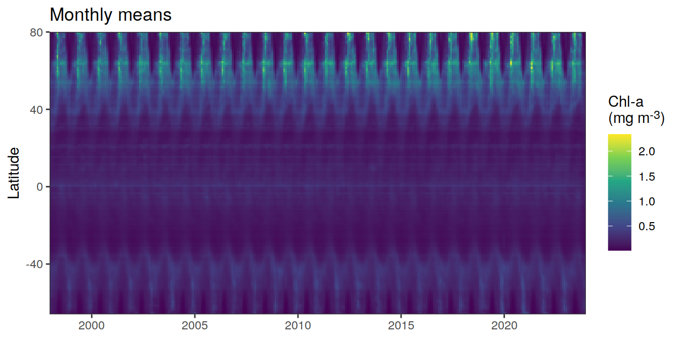
[[2]]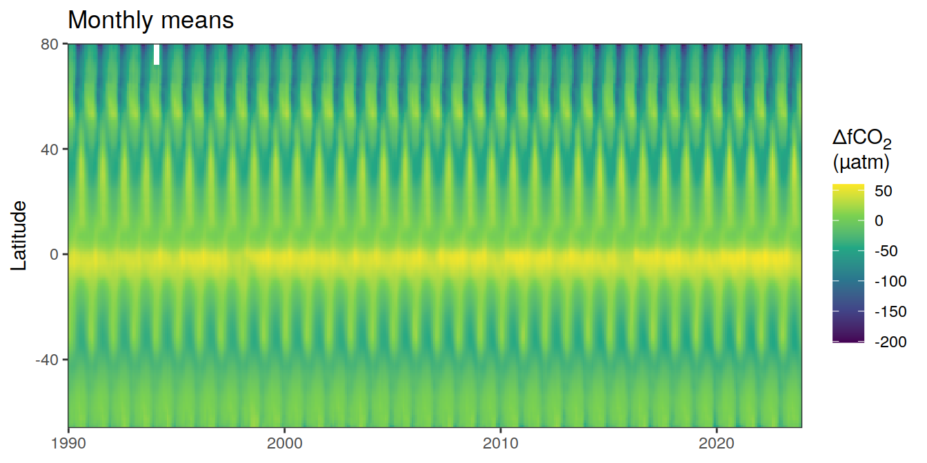
[[3]]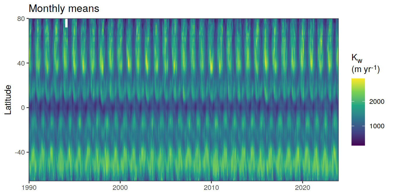
[[4]]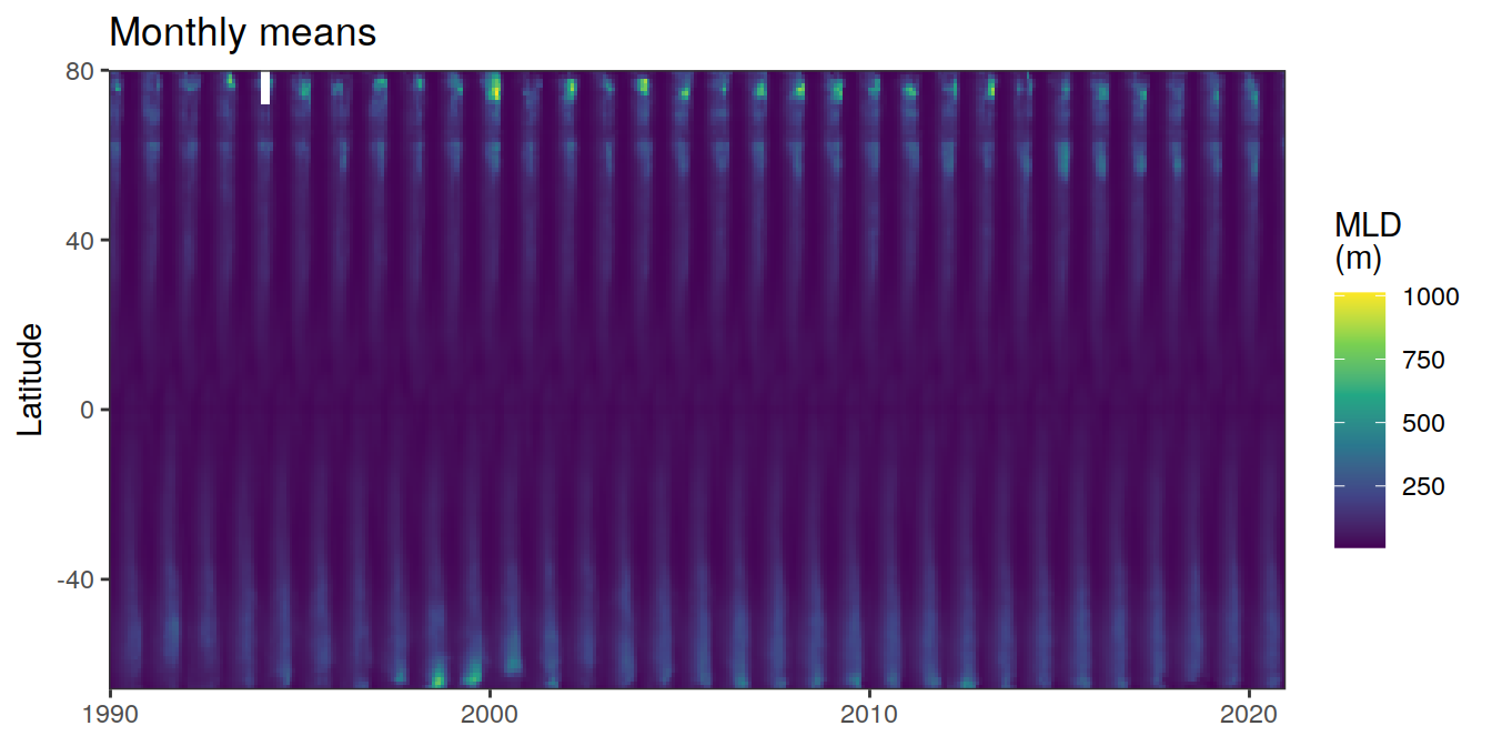
[[5]]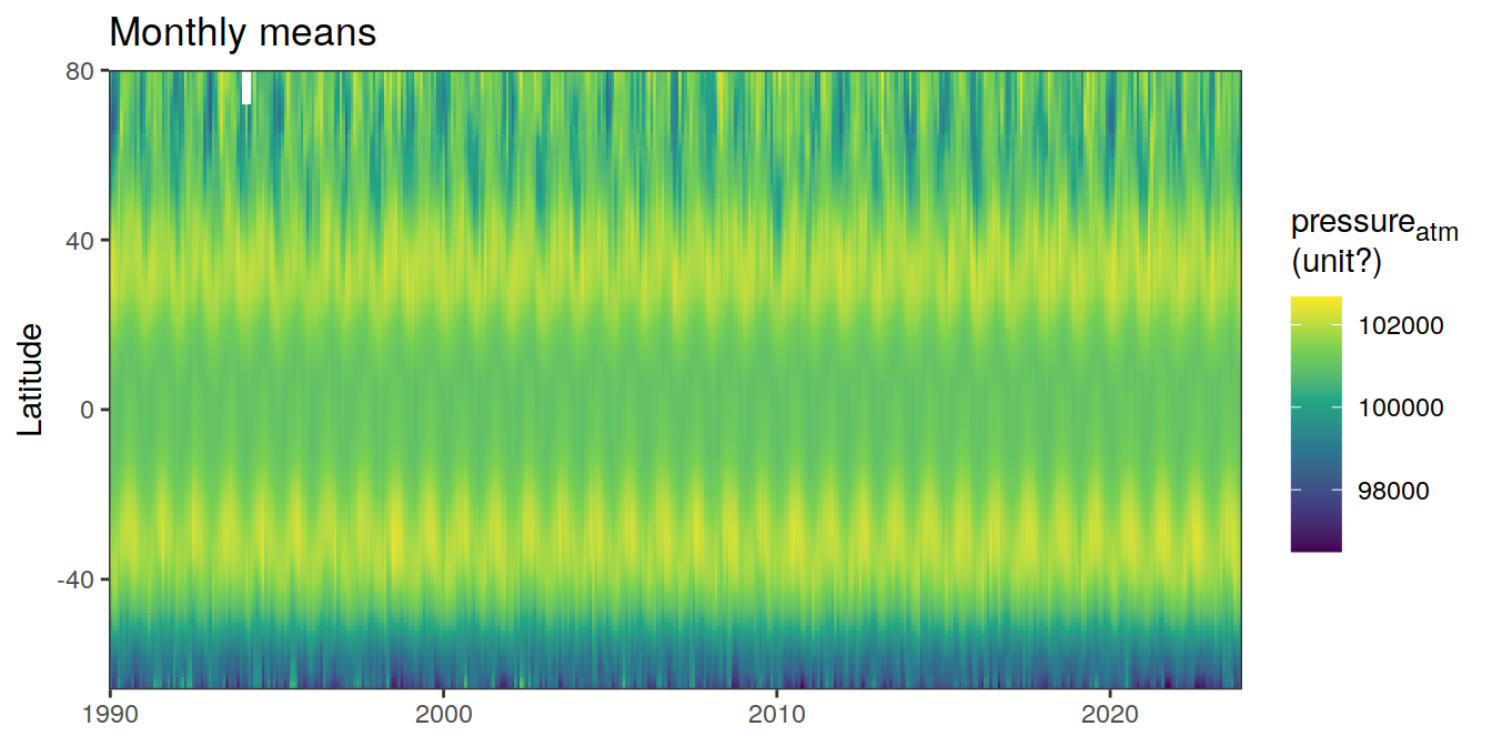
[[6]]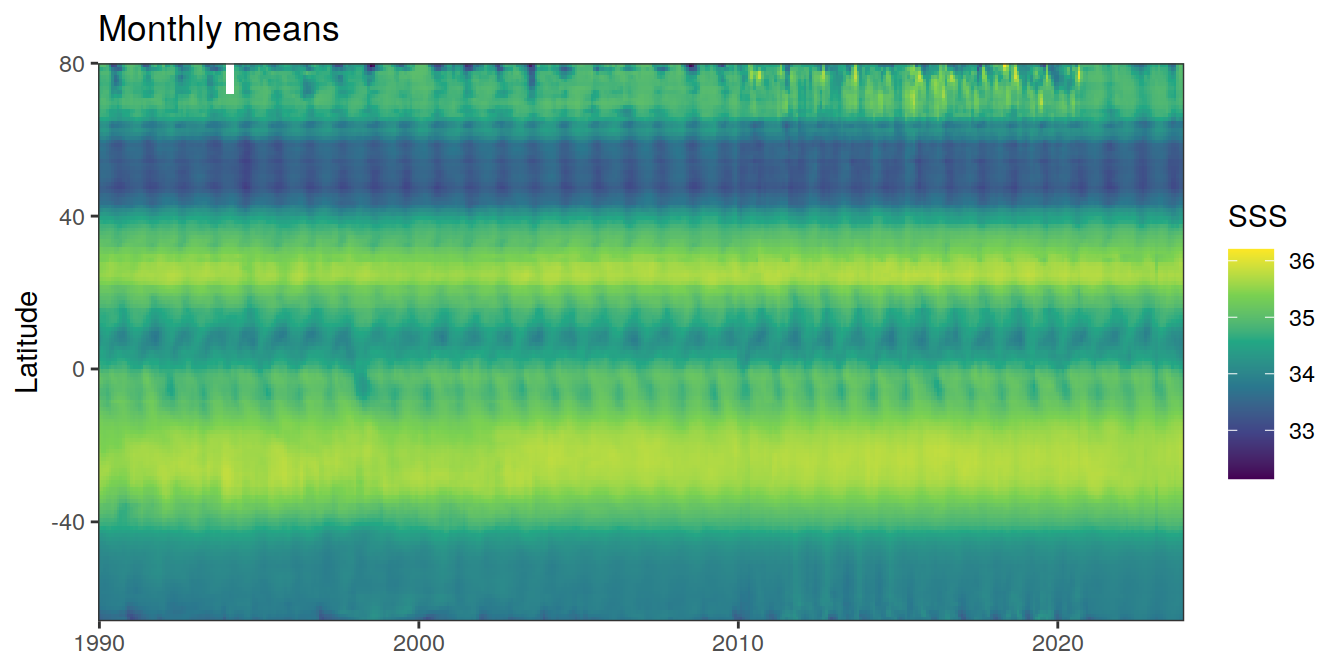
[[7]]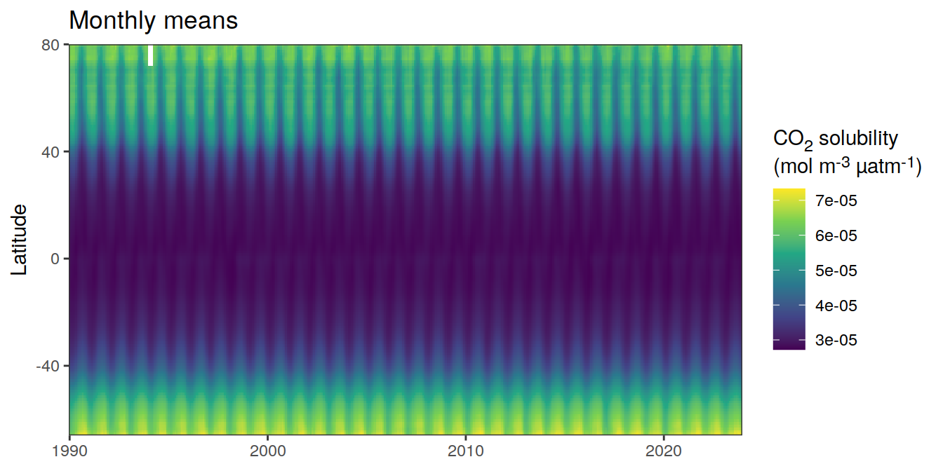
[[8]]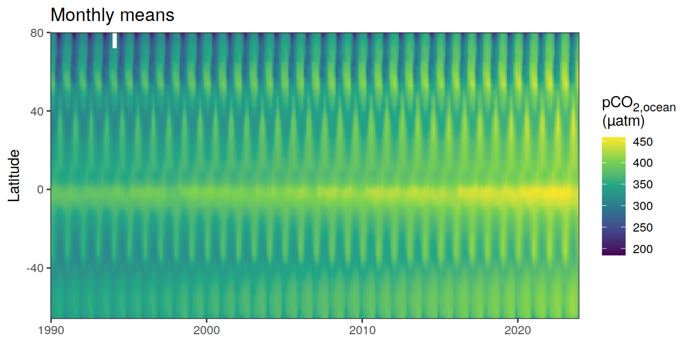
[[9]]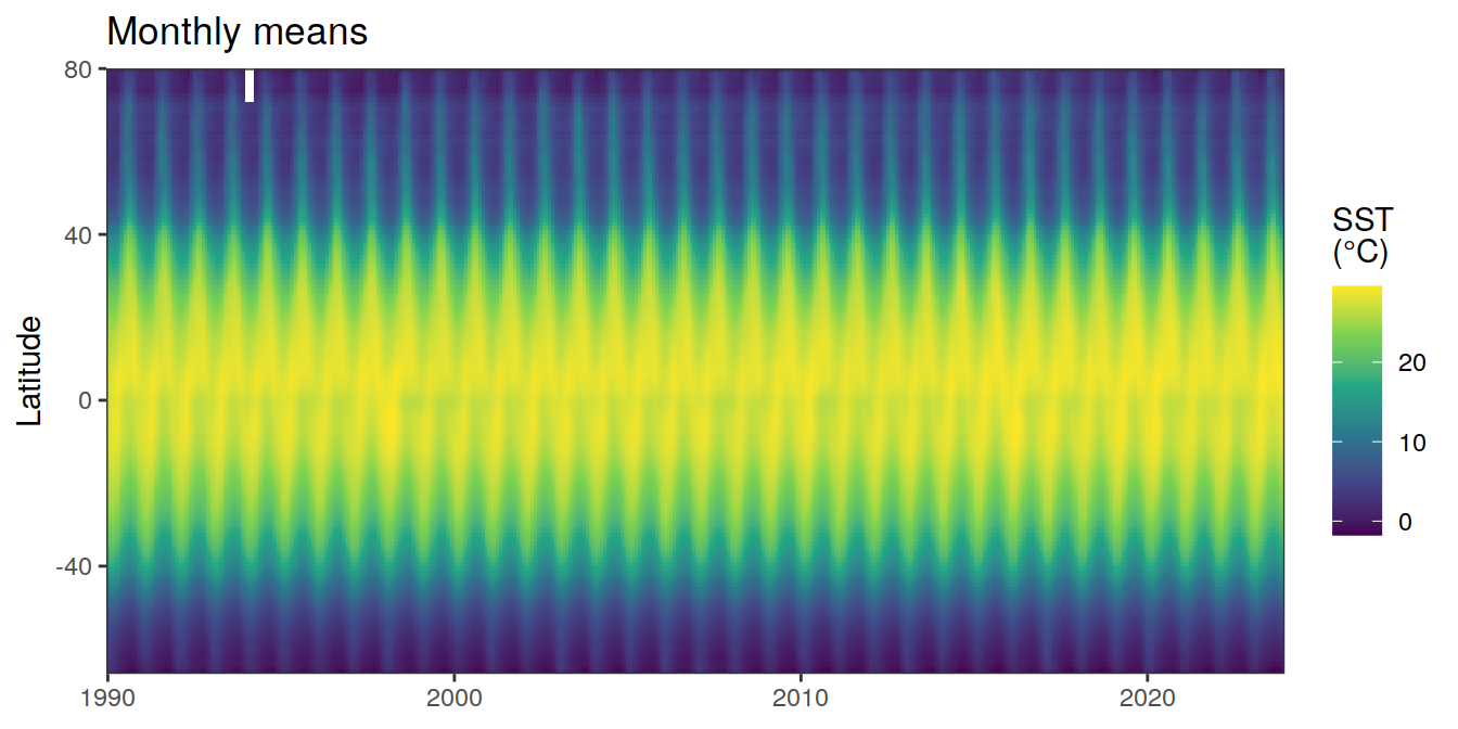
pco2_product_hovmoeller_monthly %>%
  filter(name %in% name_divergent) %>%
  group_split(name) %>%
  # head(1) %>%
  map(
    ~ ggplot(data = .x,
             aes(decimal, lat, fill = value)) +
      geom_raster() +
      scale_fill_divergent(name = labels_breaks(.x %>% distinct(name))) +
      theme(legend.title = element_markdown()) +
      labs(title = "Monthly means",
           y = "Latitude") +
      coord_cartesian(expand = 0) +
      theme(axis.title.x = element_blank())
  )
[[1]]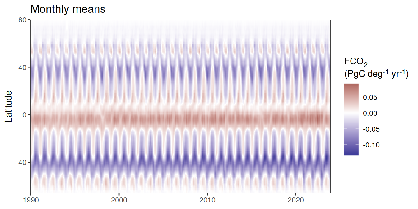
Anomalies
pco2_product_hovmoeller_monthly_regression <-
  pco2_product_hovmoeller_monthly %>%
  select(-c(decimal)) %>%
  anomaly_determination(lat, month) %>%
  filter(!is.na(resid))


pco2_product_hovmoeller_monthly_regression <-
  pco2_product_hovmoeller_monthly_regression %>%
  mutate(decimal = year + (month - 1) / 12)

pco2_product_hovmoeller_monthly_regression %>%
  group_split(name) %>%
  # head(1) %>%
  map(
    ~ ggplot(data = .x,
             aes(decimal, lat, fill = resid)) +
      geom_raster() +
      scale_fill_divergent(name = labels_breaks(.x %>% distinct(name))) +
      theme(legend.title = element_markdown()) +
      coord_cartesian(expand = 0) +
      labs(title = "Monthly mean anomalies",
           y = "Latitude") +
      theme(axis.title.x = element_blank())
  )
[[1]]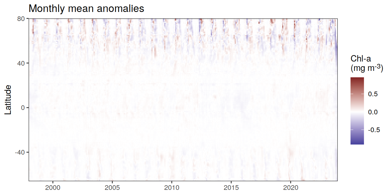
[[2]]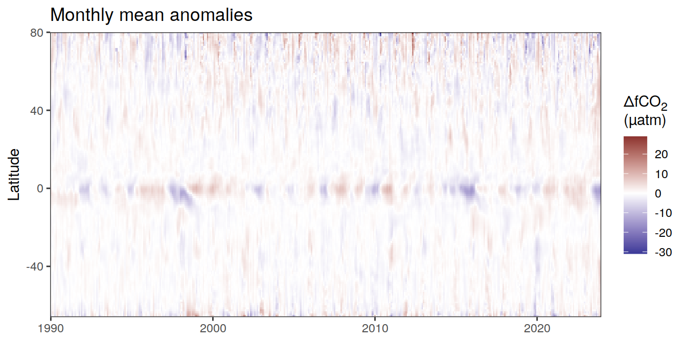
[[3]]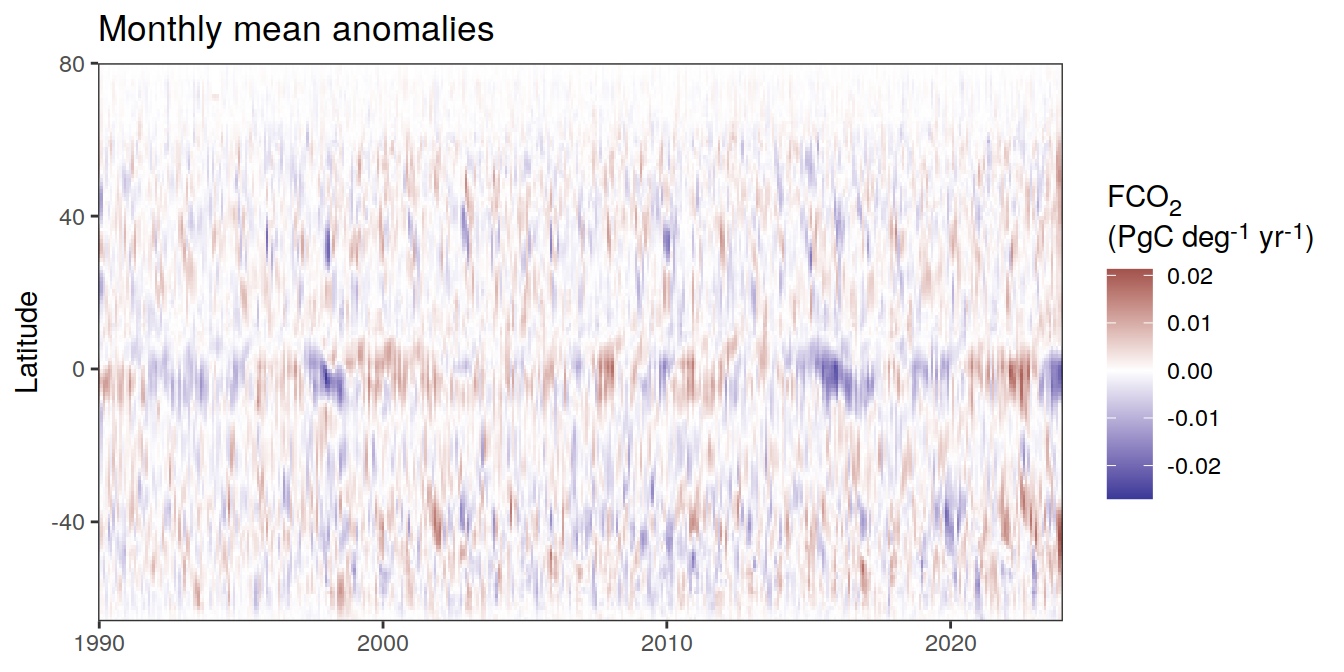
[[4]]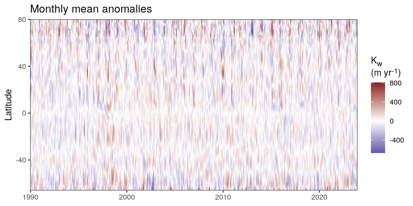
[[5]]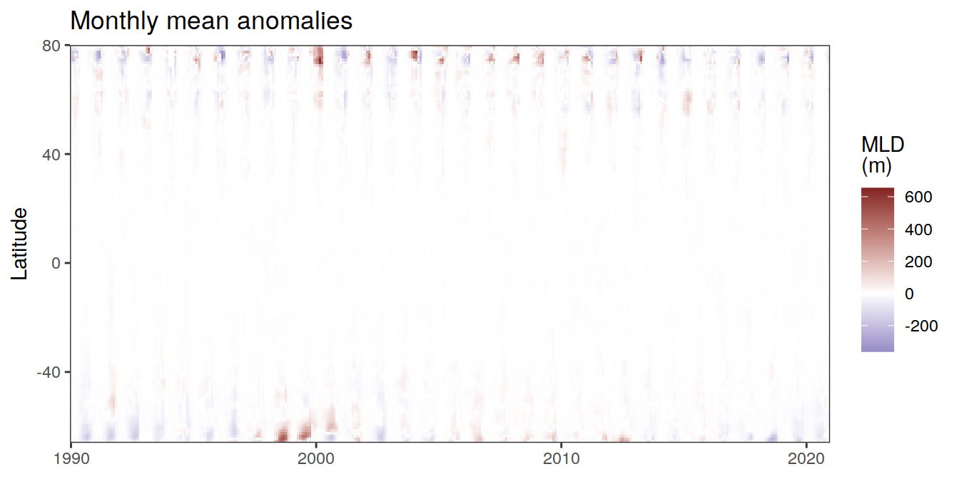
[[6]]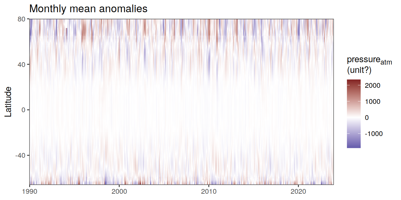
[[7]]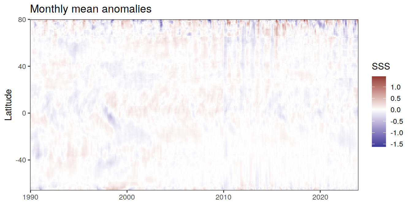
[[8]]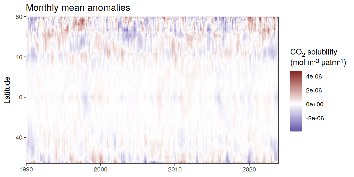
[[9]]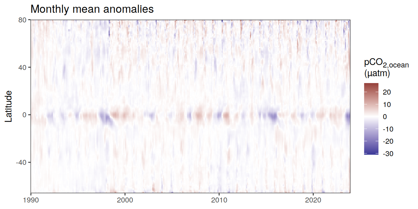
[[10]]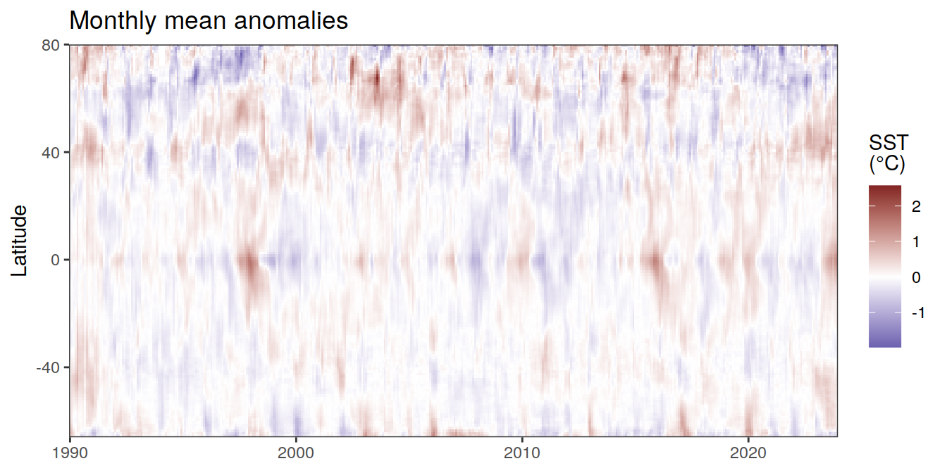
pco2_product_hovmoeller_monthly_regression %>%
  write_csv(paste0("../data/","OceanSODA","_anomaly_hovmoeller_monthly.csv"))
Anomalies since 2021
pco2_product_hovmoeller_monthly_regression %>%
  filter(year >= 2021) %>%
  group_split(name) %>%
  # head(1) %>%
  map(
    ~ ggplot(data = .x,
             aes(decimal, lat, fill = resid)) +
      geom_raster() +
      scale_fill_divergent(name = labels_breaks(.x %>% distinct(name))) +
      theme(legend.title = element_markdown()) +
      coord_cartesian(expand = 0) +
      labs(title = "Monthly mean anomalies",
           y = "Latitude") +
      theme(axis.title.x = element_blank())
  )
[[1]]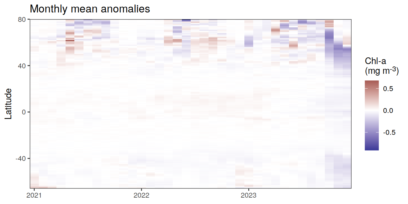
[[2]]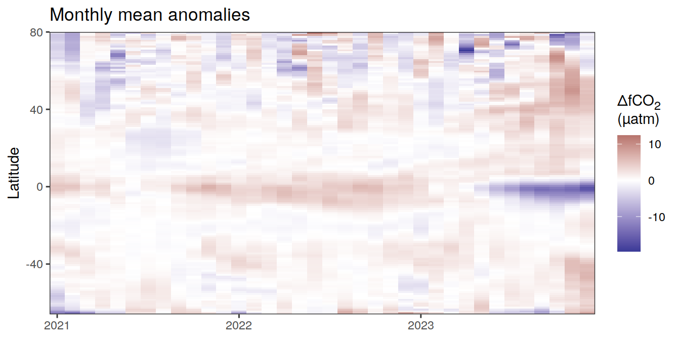
[[3]]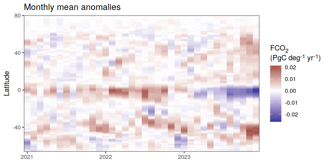
[[4]]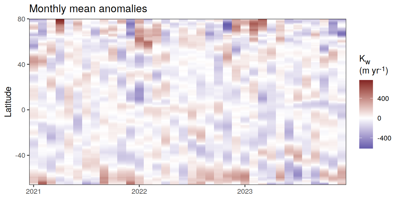
[[5]]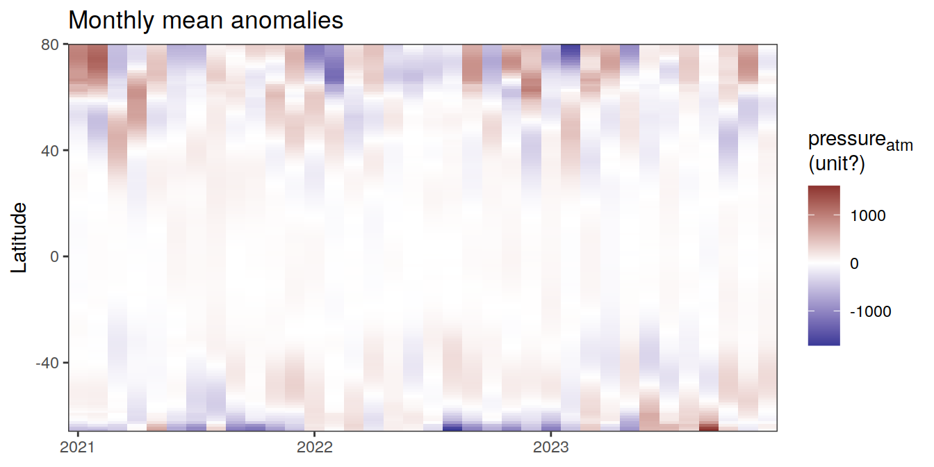
[[6]]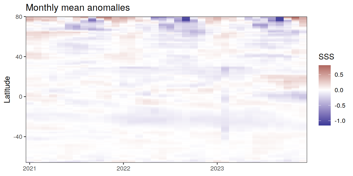
[[7]]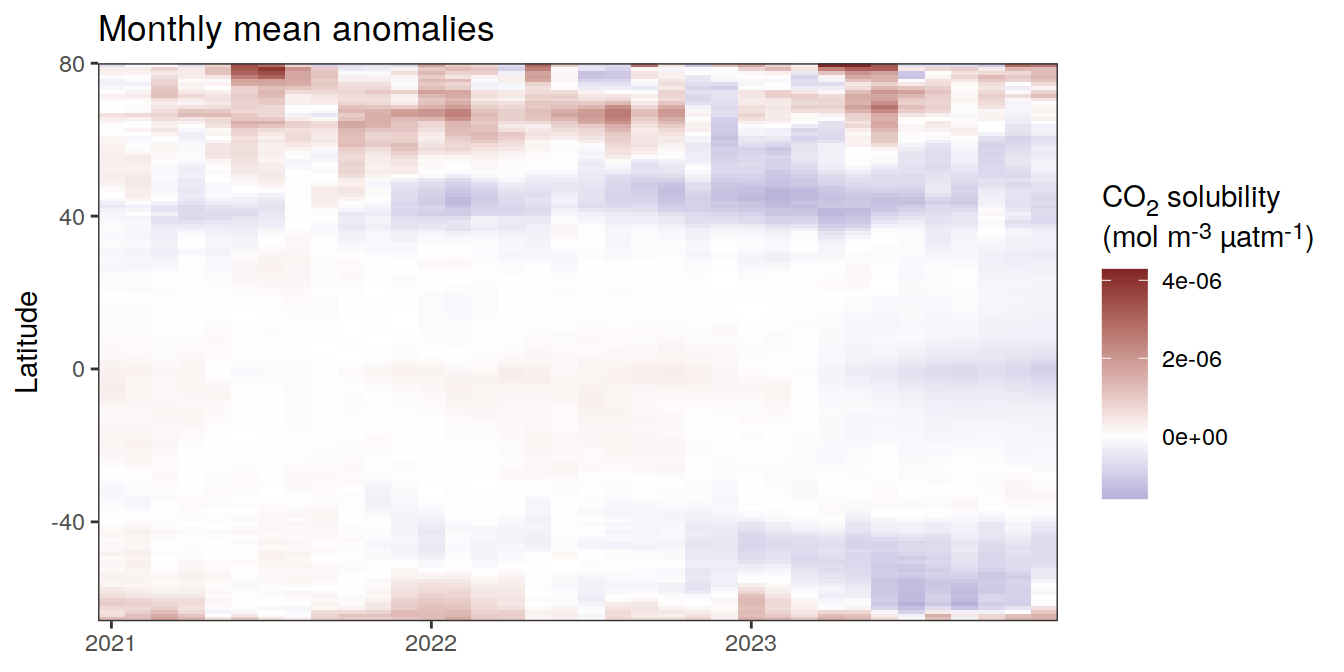
[[8]]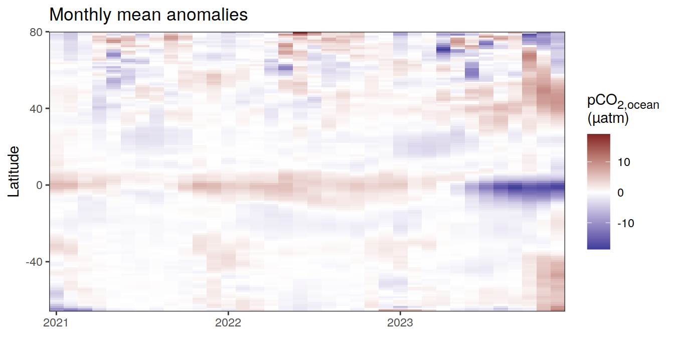
[[9]]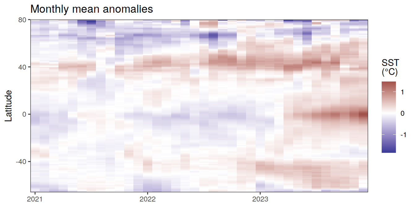
Regional means and integrals
The following plots show biome- or global- averaged/integrated values of each variable as provided through the pCO2 product, as well as the anomalies from the prediction of a linear/quadratic fit to the data from 1990 to 2022.
Anomalies are first presented relative to the predicted annual mean of each year, hence preserving the seasonality. Furthermore, anomalies are presented relative to the predicted monthly mean values, such that the mean seasonality is removed.
pco2_product_monthly_global <-
  pco2_product %>%
  select(-c(lon, lat, year, month, biome)) %>%
  group_by(time) %>%
  summarise(across(-c(fgco2, area),
                   ~ weighted.mean(., area, na.rm = TRUE)),
            across(fgco2,
                   ~ sum(. * area, na.rm = TRUE) * 12.01 * 1e-15)) %>%
  ungroup()

pco2_product_monthly_biome <-
  pco2_product %>%
  select(-c(lon, lat, year, month)) %>%
  group_by(time, biome) %>%
  summarise(across(-c(fgco2, area),
                   ~ weighted.mean(., area, na.rm = TRUE)),
            across(fgco2,
                   ~ sum(. * area, na.rm = TRUE) * 12.01 * 1e-15)) %>%
  ungroup()

pco2_product_monthly_biome_super <-
  pco2_product %>%
  mutate(
    biome = case_when(
      str_detect(biome, "NA-") ~ "North Atlantic",
      str_detect(biome, "NP-") ~ "North Pacific",
      str_detect(biome, "SO-") ~ "Southern Ocean",
      TRUE ~ "other"
    )
  ) %>%
  filter(biome != "other") %>%
  select(-c(lon, lat, year, month)) %>%
  group_by(time, biome) %>%
  summarise(across(-c(fgco2, area),
                   ~ weighted.mean(., area, na.rm = TRUE)),
            across(fgco2,
                   ~ sum(. * area, na.rm = TRUE) * 12.01 * 1e-15)) %>%
  ungroup()

pco2_product_monthly <-
  bind_rows(pco2_product_monthly_global %>%
              mutate(biome = "Global"),
            pco2_product_monthly_biome,
            pco2_product_monthly_biome_super)

rm(
  pco2_product_monthly_global,
  pco2_product_monthly_biome,
  pco2_product_monthly_biome_super
)


pco2_product_monthly <-
  pco2_product_monthly %>%
  filter(!is.na(biome))

pco2_product_monthly <-
  pco2_product_monthly %>%
  rename(fgco2_int = fgco2)

pco2_product_monthly <-
  pco2_product_monthly %>%
  mutate(year = year(time),
         month = month(time),
         .after = time)

pco2_product_monthly <-
  pco2_product_monthly %>%
  pivot_longer(-c(time, year, month, biome))
Absolute values
Overview
fig.height <- pco2_product_monthly %>%
  distinct(name) %>%
  nrow() * 0.15
pco2_product_monthly %>%
filter(biome %in% "Global") %>%
ggplot(aes(month, value, group = as.factor(year))) +
geom_path(data = . %>% filter(year < 2022),
aes(col = year)) +
scale_color_grayC() +
new_scale_color() +
geom_path(data = . %>% filter(year >= 2022),
aes(col = as.factor(year)),
linewidth = 1) +
scale_color_manual(values = c("orange", "red"),
guide = guide_legend(reverse = TRUE,
order = 1)) +
scale_x_continuous(breaks = seq(1, 12, 3), expand = c(0, 0)) +
labs(title = "Absolute values | Global") +
facet_wrap(name ~ .,
scales = "free_y",
labeller = labeller(name = x_axis_labels),
strip.position = "left",
ncol = 2) +
theme(
strip.text.y.left = element_markdown(),
strip.placement = "outside",
strip.background.y = element_blank(),
legend.title = element_blank(),
axis.title.y = element_blank()
)
| Version | Author | Date |
|---|---|---|
| 2fdbfec | jens-daniel-mueller | 2024-03-21 |
| 83fcd67 | jens-daniel-mueller | 2024-03-21 |
| 342018b | jens-daniel-mueller | 2024-03-20 |
| f0a1de7 | jens-daniel-mueller | 2024-03-20 |
| 2d2fb75 | jens-daniel-mueller | 2024-03-20 |
| d520917 | jens-daniel-mueller | 2024-03-19 |
| 03321bd | jens-daniel-mueller | 2024-03-19 |
| b41fa51 | jens-daniel-mueller | 2024-03-19 |
pco2_product_monthly %>%
  filter(biome %in% key_biomes) %>%
  ggplot(aes(month, value, group = as.factor(year))) +
  geom_path(data = . %>% filter(year < 2022),
            aes(col = year)) +
  scale_color_grayC() +
  new_scale_color() +
  geom_path(data = . %>% filter(year >= 2022),
            aes(col = as.factor(year)),
            linewidth = 1) +
  scale_color_manual(values = c("orange", "red"),
                     guide = guide_legend(reverse = TRUE,
                                          order = 1)) +
  scale_x_continuous(breaks = seq(1, 12, 3), expand = c(0, 0)) +
  labs(title = "Absolute values | Selected biomes") +
  facet_grid(name ~ biome,
             scales = "free_y",
             labeller = labeller(name = x_axis_labels),
             switch = "y") +
  theme(
    strip.text.y.left = element_markdown(),
    strip.placement = "outside",
    strip.background.y = element_blank(),
    legend.title = element_blank(),
    axis.title.y = element_blank()
  )
| Version | Author | Date |
|---|---|---|
| e3e1491 | jens-daniel-mueller | 2024-03-21 |
pco2_product_monthly %>%
  filter(biome %in% super_biomes) %>%
  ggplot(aes(month, value, group = as.factor(year))) +
  geom_path(data = . %>% filter(year < 2022),
            aes(col = year)) +
  scale_color_grayC() +
  new_scale_color() +
  geom_path(data = . %>% filter(year >= 2022),
            aes(col = as.factor(year)),
            linewidth = 1) +
  scale_color_manual(values = c("orange", "red"),
                     guide = guide_legend(reverse = TRUE,
                                          order = 1)) +
  scale_x_continuous(breaks = seq(1, 12, 3), expand = c(0, 0)) +
  labs(title = "Absolute values | Selected super biomes") +
  facet_grid(name ~ biome,
             scales = "free_y",
             labeller = labeller(name = x_axis_labels),
             switch = "y") +
  theme(
    strip.text.y.left = element_markdown(),
    strip.placement = "outside",
    strip.background.y = element_blank(),
    legend.title = element_blank(),
    axis.title.y = element_blank()
  )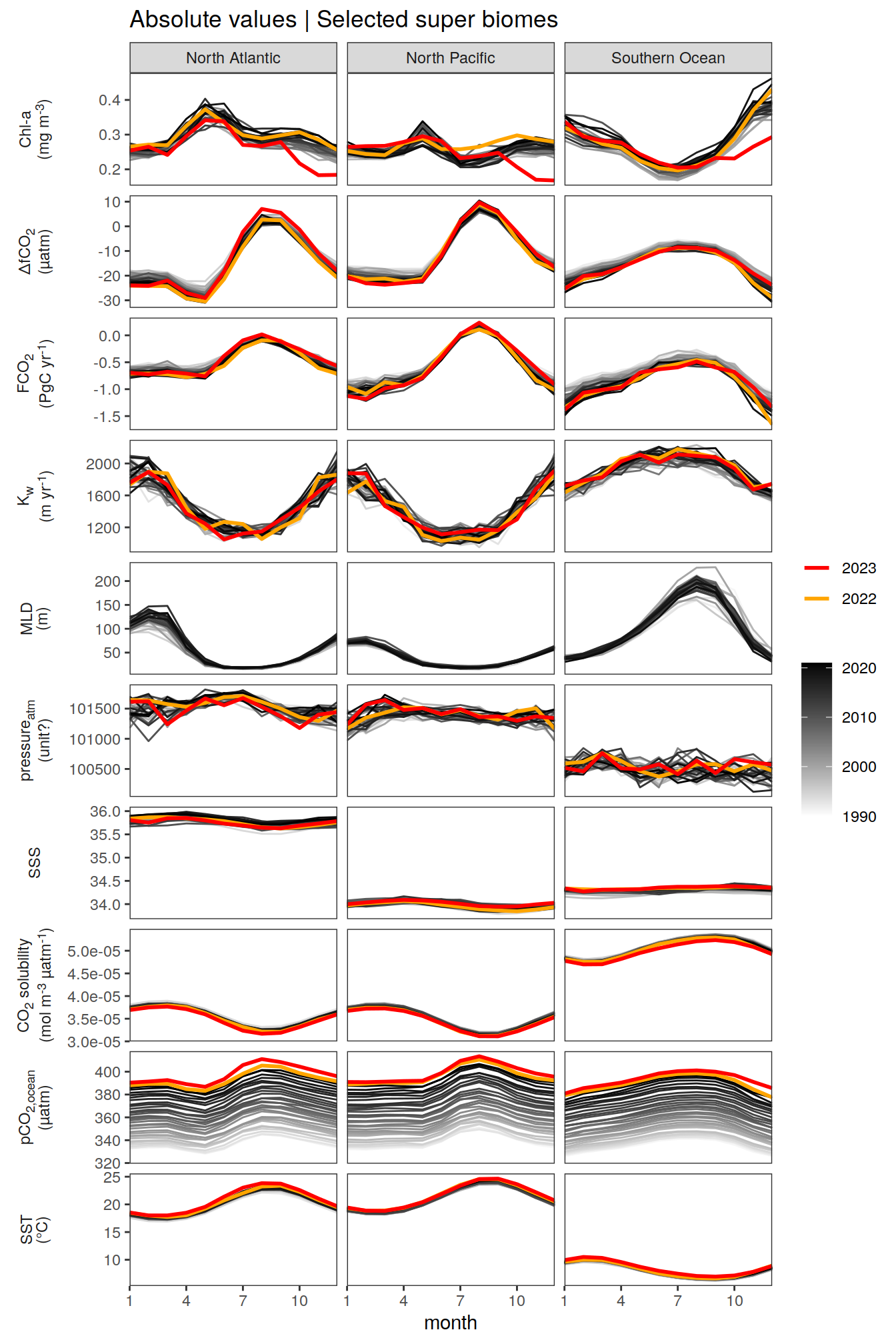
| Version | Author | Date |
|---|---|---|
| e3e1491 | jens-daniel-mueller | 2024-03-21 |
Selected biomes
pco2_product_monthly %>%
  filter(biome %in% key_biomes) %>%
  group_split(biome) %>%
  # head(1) %>%
  map(
    ~ ggplot(data = .x,
             aes(month, value, group = as.factor(year))) +
      geom_path(data = . %>% filter(year < 2022),
                aes(col = year)) +
      scale_color_grayC() +
      new_scale_color() +
      geom_path(
        data = . %>% filter(year >= 2022),
        aes(col = as.factor(year)),
        linewidth = 1
      ) +
      scale_color_manual(
        values = c("orange", "red"),
        guide = guide_legend(reverse = TRUE,
                             order = 1)
      ) +
      scale_x_continuous(breaks = seq(1, 12, 3), expand = c(0, 0)) +
  labs(title = paste("Absolute values |", .x$biome)) +
  facet_wrap(name ~ .,
             scales = "free_y",
             labeller = labeller(name = x_axis_labels),
             strip.position = "left",
             ncol = 2) +
  theme(
    strip.text.y.left = element_markdown(),
    strip.placement = "outside",
    strip.background.y = element_blank(),
    legend.title = element_blank(),
    axis.title.y = element_blank()
  )
  )
[[1]]
| Version | Author | Date |
|---|---|---|
| 2fdbfec | jens-daniel-mueller | 2024-03-21 |
| 83fcd67 | jens-daniel-mueller | 2024-03-21 |
| 342018b | jens-daniel-mueller | 2024-03-20 |
| f0a1de7 | jens-daniel-mueller | 2024-03-20 |
| 2d2fb75 | jens-daniel-mueller | 2024-03-20 |
| d520917 | jens-daniel-mueller | 2024-03-19 |
| 03321bd | jens-daniel-mueller | 2024-03-19 |
| b41fa51 | jens-daniel-mueller | 2024-03-19 |
[[2]]
| Version | Author | Date |
|---|---|---|
| 2fdbfec | jens-daniel-mueller | 2024-03-21 |
| 83fcd67 | jens-daniel-mueller | 2024-03-21 |
| 342018b | jens-daniel-mueller | 2024-03-20 |
| f0a1de7 | jens-daniel-mueller | 2024-03-20 |
| 2d2fb75 | jens-daniel-mueller | 2024-03-20 |
| d520917 | jens-daniel-mueller | 2024-03-19 |
| 03321bd | jens-daniel-mueller | 2024-03-19 |
| b41fa51 | jens-daniel-mueller | 2024-03-19 |
[[3]]
| Version | Author | Date |
|---|---|---|
| 2fdbfec | jens-daniel-mueller | 2024-03-21 |
| 83fcd67 | jens-daniel-mueller | 2024-03-21 |
| 342018b | jens-daniel-mueller | 2024-03-20 |
| f0a1de7 | jens-daniel-mueller | 2024-03-20 |
| 2d2fb75 | jens-daniel-mueller | 2024-03-20 |
| d520917 | jens-daniel-mueller | 2024-03-19 |
| 03321bd | jens-daniel-mueller | 2024-03-19 |
| b41fa51 | jens-daniel-mueller | 2024-03-19 |
[[4]]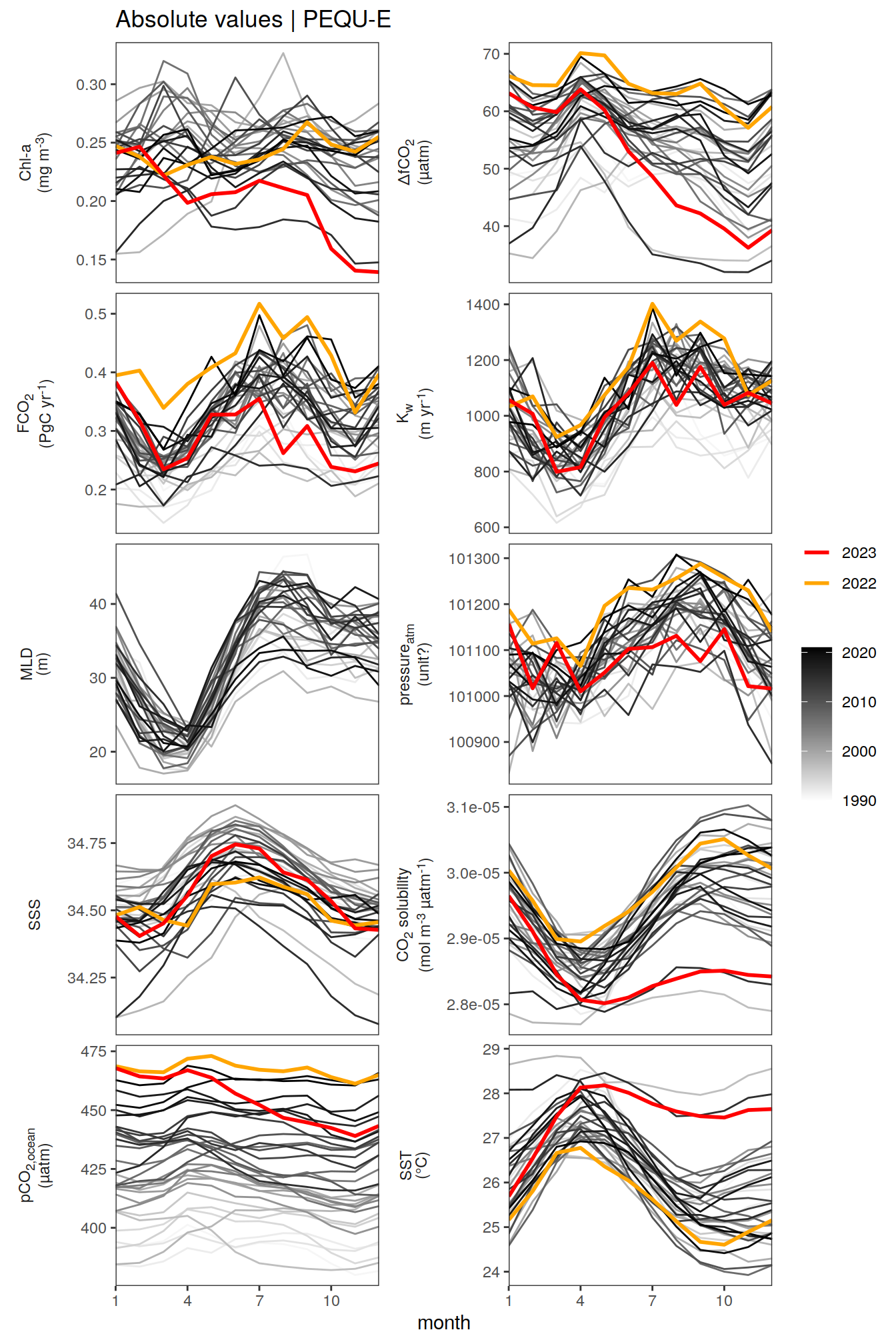
| Version | Author | Date |
|---|---|---|
| 2fdbfec | jens-daniel-mueller | 2024-03-21 |
| 83fcd67 | jens-daniel-mueller | 2024-03-21 |
| 342018b | jens-daniel-mueller | 2024-03-20 |
| f0a1de7 | jens-daniel-mueller | 2024-03-20 |
| 2d2fb75 | jens-daniel-mueller | 2024-03-20 |
| d520917 | jens-daniel-mueller | 2024-03-19 |
| 03321bd | jens-daniel-mueller | 2024-03-19 |
| b41fa51 | jens-daniel-mueller | 2024-03-19 |
[[5]]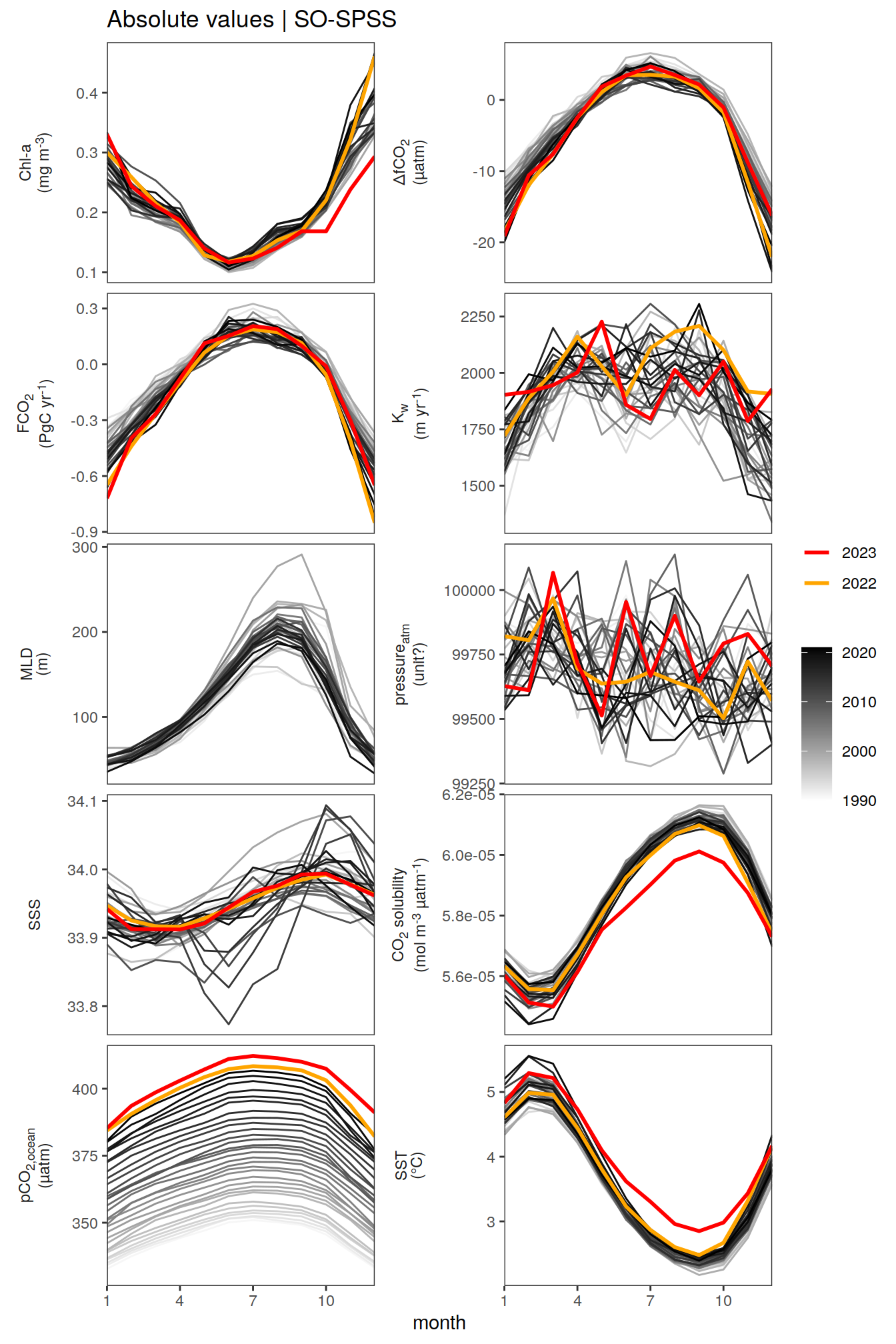
| Version | Author | Date |
|---|---|---|
| 2fdbfec | jens-daniel-mueller | 2024-03-21 |
| 83fcd67 | jens-daniel-mueller | 2024-03-21 |
| 342018b | jens-daniel-mueller | 2024-03-20 |
| f0a1de7 | jens-daniel-mueller | 2024-03-20 |
| 2d2fb75 | jens-daniel-mueller | 2024-03-20 |
| d520917 | jens-daniel-mueller | 2024-03-19 |
| 03321bd | jens-daniel-mueller | 2024-03-19 |
| b41fa51 | jens-daniel-mueller | 2024-03-19 |
Super biomes
pco2_product_monthly %>%
  filter(biome %in% super_biomes) %>%
  group_split(biome) %>%
  # head(1) %>%
  map(
    ~ ggplot(data = .x,
             aes(month, value, group = as.factor(year))) +
      geom_path(data = . %>% filter(year < 2022),
                aes(col = year)) +
      scale_color_grayC() +
      new_scale_color() +
      geom_path(
        data = . %>% filter(year >= 2022),
        aes(col = as.factor(year)),
        linewidth = 1
      ) +
      scale_color_manual(
        values = c("orange", "red"),
        guide = guide_legend(reverse = TRUE,
                             order = 1)
      ) +
      scale_x_continuous(breaks = seq(1, 12, 3), expand = c(0, 0)) +
  labs(title = paste("Absolute values |", .x$biome)) +
  facet_wrap(name ~ .,
             scales = "free_y",
             labeller = labeller(name = x_axis_labels),
             strip.position = "left",
             ncol = 2) +
  theme(
    strip.text.y.left = element_markdown(),
    strip.placement = "outside",
    strip.background.y = element_blank(),
    legend.title = element_blank(),
    axis.title.y = element_blank()
  )
  )
[[1]]
| Version | Author | Date |
|---|---|---|
| e3e1491 | jens-daniel-mueller | 2024-03-21 |
[[2]]
| Version | Author | Date |
|---|---|---|
| e3e1491 | jens-daniel-mueller | 2024-03-21 |
[[3]]
| Version | Author | Date |
|---|---|---|
| e3e1491 | jens-daniel-mueller | 2024-03-21 |
Anomalies
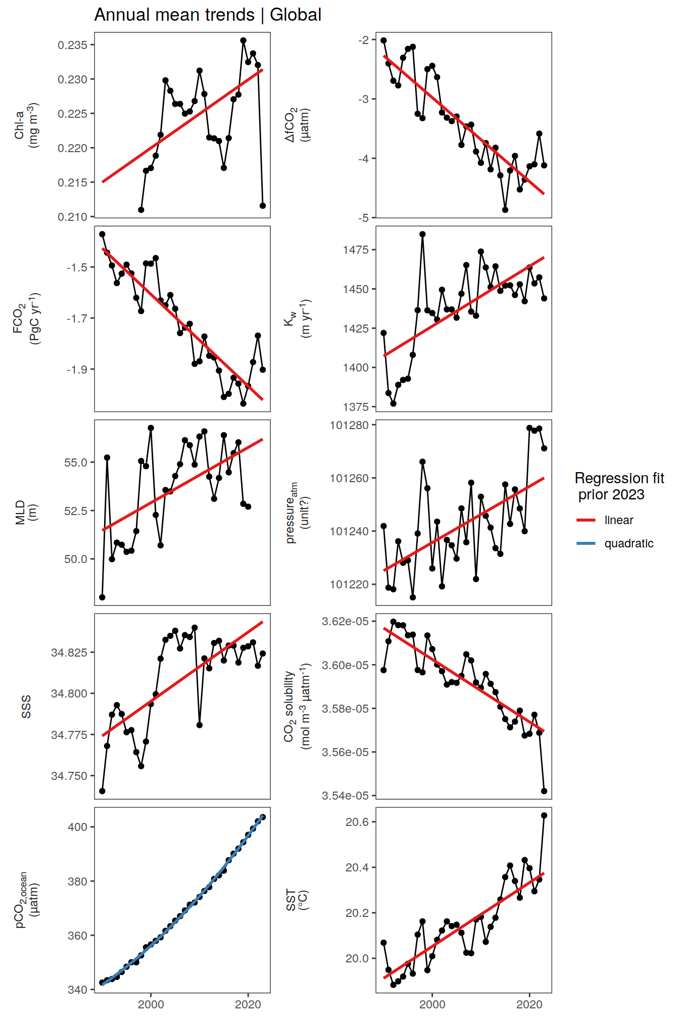
Annual mean trends
pco2_product_annual <-
  pco2_product_monthly %>%
  group_by(year, biome, name) %>%
  summarise(value = mean(value)) %>%
  ungroup()

pco2_product_annual %>%
  filter(biome %in% "Global") %>%
  ggplot(aes(year, value)) +
  geom_path() +
  geom_point() +
  geom_smooth(data = . %>% filter(year <= 2022,
                                  !(name %in% name_quadratic_fit)),
              method = "lm",
              fullrange = TRUE,
              aes(col = "linear"),
              se = FALSE) +
  geom_smooth(data = . %>% filter(year <= 2022,
                                  name %in% name_quadratic_fit),
              method = "lm",
              fullrange = TRUE,
              formula = y ~ x + I(x^2),
              aes(col = "quadratic"),
              se = FALSE) +
  scale_color_brewer(
    palette = "Set1",
    name = "Regression fit\n prior 2023") +
  scale_x_continuous(breaks = seq(1980, 2020, 20)) +
  labs(title = "Annual mean trends | Global") +
  facet_wrap(name ~ .,
             scales = "free_y",
             labeller = labeller(name = x_axis_labels),
             strip.position = "left",
             ncol = 2) +
  theme(
    strip.text.y.left = element_markdown(),
    strip.placement = "outside",
    strip.background.y = element_blank(),
    axis.title = element_blank()
  )
| Version | Author | Date |
|---|---|---|
| 2fdbfec | jens-daniel-mueller | 2024-03-21 |
| 83fcd67 | jens-daniel-mueller | 2024-03-21 |
| 342018b | jens-daniel-mueller | 2024-03-20 |
| f0a1de7 | jens-daniel-mueller | 2024-03-20 |
| 2d2fb75 | jens-daniel-mueller | 2024-03-20 |
| d520917 | jens-daniel-mueller | 2024-03-19 |
| 03321bd | jens-daniel-mueller | 2024-03-19 |
| b41fa51 | jens-daniel-mueller | 2024-03-19 |
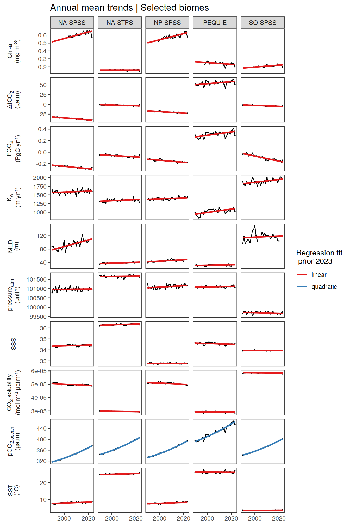
pco2_product_annual %>%
  filter(biome %in% key_biomes) %>%
  ggplot(aes(year, value)) +
  geom_path() +
  geom_point(size = 0.2) +
  geom_smooth(data = . %>% filter(year <= 2022,
                                  !(name %in% name_quadratic_fit)),
              method = "lm",
              fullrange = TRUE,
              aes(col = "linear"),
              se = FALSE) +
  geom_smooth(data = . %>% filter(year <= 2022,
                                  name %in% name_quadratic_fit),
              method = "lm",
              fullrange = TRUE,
              formula = y ~ x + I(x^2),
              aes(col = "quadratic"),
              se = FALSE) +
  scale_color_brewer(
    palette = "Set1",
    name = "Regression fit\n prior 2023") +
  scale_x_continuous(breaks = seq(1980, 2020, 20)) +
  labs(title = "Annual mean trends | Selected biomes") +
  facet_grid(name ~ biome,
             scales = "free_y",
             labeller = labeller(name = x_axis_labels),
             switch = "y") +
  theme(
    strip.text.y.left = element_markdown(),
    strip.placement = "outside",
    strip.background.y = element_blank(),
    axis.title = element_blank()
  )
| Version | Author | Date |
|---|---|---|
| 2fdbfec | jens-daniel-mueller | 2024-03-21 |
| 83fcd67 | jens-daniel-mueller | 2024-03-21 |
| 342018b | jens-daniel-mueller | 2024-03-20 |
| f0a1de7 | jens-daniel-mueller | 2024-03-20 |
| 2d2fb75 | jens-daniel-mueller | 2024-03-20 |
| d520917 | jens-daniel-mueller | 2024-03-19 |
| 03321bd | jens-daniel-mueller | 2024-03-19 |
| b41fa51 | jens-daniel-mueller | 2024-03-19 |
pco2_product_annual %>%
  filter(biome %in% super_biomes) %>%
  ggplot(aes(year, value)) +
  geom_path() +
  geom_point(size = 0.2) +
  geom_smooth(data = . %>% filter(year <= 2022,
                                  !(name %in% name_quadratic_fit)),
              method = "lm",
              fullrange = TRUE,
              aes(col = "linear"),
              se = FALSE) +
  geom_smooth(data = . %>% filter(year <= 2022,
                                  name %in% name_quadratic_fit),
              method = "lm",
              fullrange = TRUE,
              formula = y ~ x + I(x^2),
              aes(col = "quadratic"),
              se = FALSE) +
  scale_color_brewer(
    palette = "Set1",
    name = "Regression fit\n prior 2023") +
  scale_x_continuous(breaks = seq(1980, 2020, 20)) +
  labs(title = "Annual mean trends | Selected super biomes") +
  facet_grid(name ~ biome,
             scales = "free_y",
             labeller = labeller(name = x_axis_labels),
             switch = "y") +
  theme(
    strip.text.y.left = element_markdown(),
    strip.placement = "outside",
    strip.background.y = element_blank(),
    axis.title = element_blank()
  )
| Version | Author | Date |
|---|---|---|
| e3e1491 | jens-daniel-mueller | 2024-03-21 |
| 2fdbfec | jens-daniel-mueller | 2024-03-21 |
| 83fcd67 | jens-daniel-mueller | 2024-03-21 |
| 342018b | jens-daniel-mueller | 2024-03-20 |
| f0a1de7 | jens-daniel-mueller | 2024-03-20 |
| 2d2fb75 | jens-daniel-mueller | 2024-03-20 |
| d520917 | jens-daniel-mueller | 2024-03-19 |
| 03321bd | jens-daniel-mueller | 2024-03-19 |
| b41fa51 | jens-daniel-mueller | 2024-03-19 |
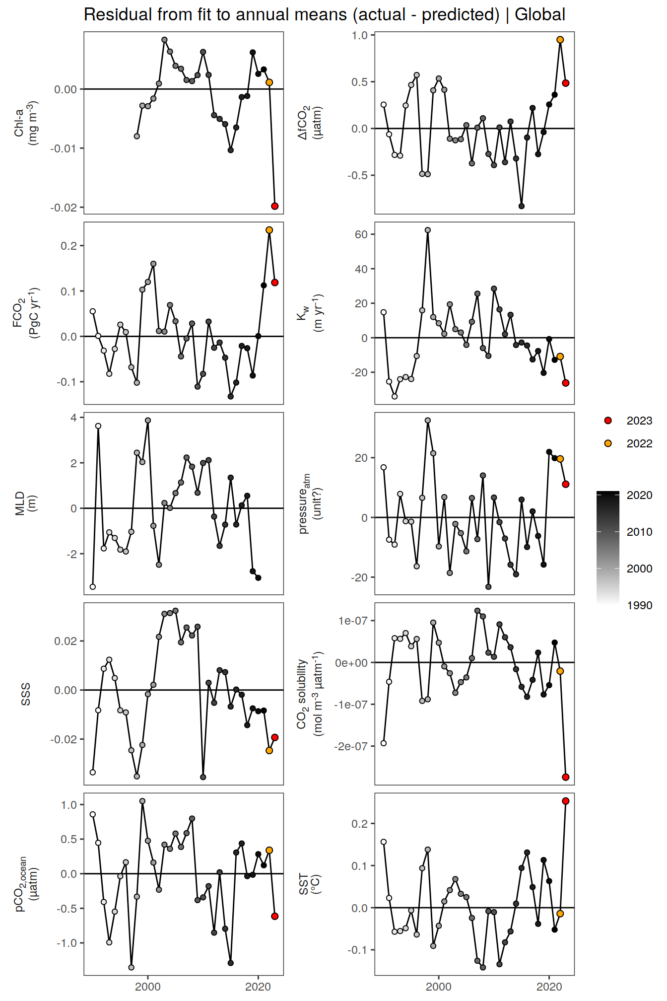
pco2_product_annual_regression <-
  pco2_product_annual %>%
  anomaly_determination(biome)


pco2_product_annual_regression %>%
  filter(biome %in% "Global") %>%
  ggplot(aes(year, resid)) +
  geom_hline(yintercept = 0) +
  geom_path() +
  geom_point(data = . %>% filter(year < 2022),
             aes(fill = year),
             shape = 21) +
  scale_fill_grayC() +
  new_scale_fill() +
  geom_point(data = . %>% filter(year >= 2022),
             aes(fill = as.factor(year)),
             shape = 21, size = 2)  +
  scale_fill_manual(values = c("orange", "red"),
                     guide = guide_legend(reverse = TRUE,
                                          order = 1)) +
  scale_x_continuous(breaks = seq(1980, 2020, 20)) +
  labs(title = "Residual from fit to annual means (actual - predicted) | Global") +
  facet_wrap(name ~ .,
             scales = "free_y",
             labeller = labeller(name = x_axis_labels),
             strip.position = "left",
             ncol = 2) +
  theme(
    strip.text.y.left = element_markdown(),
    strip.placement = "outside",
    strip.background.y = element_blank(),
    axis.title = element_blank(),
    legend.title = element_blank()
  )
| Version | Author | Date |
|---|---|---|
| e3e1491 | jens-daniel-mueller | 2024-03-21 |
| 2fdbfec | jens-daniel-mueller | 2024-03-21 |
| 83fcd67 | jens-daniel-mueller | 2024-03-21 |
| 342018b | jens-daniel-mueller | 2024-03-20 |
| f0a1de7 | jens-daniel-mueller | 2024-03-20 |
| 2d2fb75 | jens-daniel-mueller | 2024-03-20 |
| d520917 | jens-daniel-mueller | 2024-03-19 |
| 03321bd | jens-daniel-mueller | 2024-03-19 |
| b41fa51 | jens-daniel-mueller | 2024-03-19 |
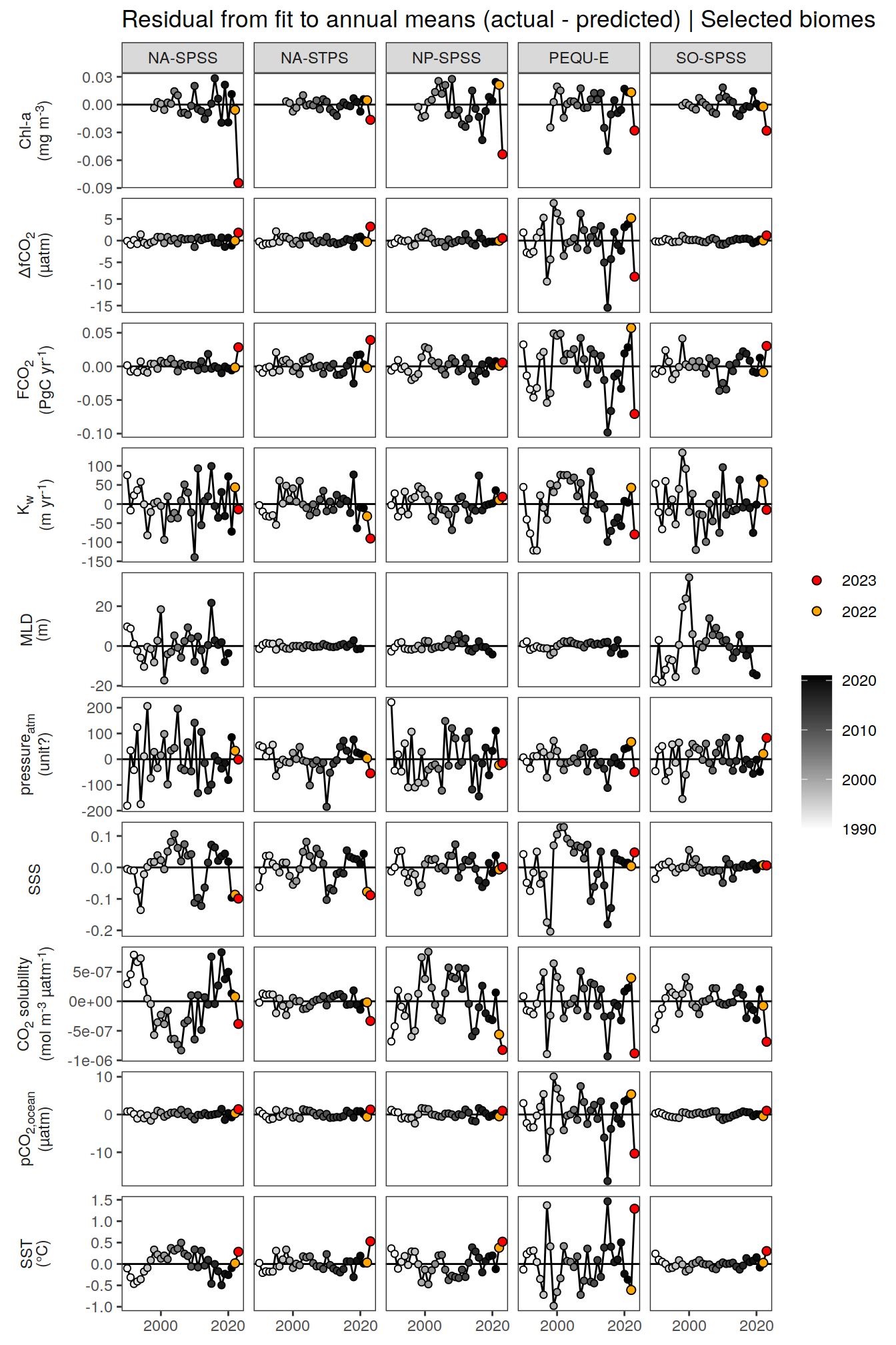
pco2_product_annual_regression %>%
  filter(biome %in% key_biomes) %>%
  ggplot(aes(year, resid)) +
  geom_hline(yintercept = 0) +
  geom_path() +
  geom_point(data = . %>% filter(year < 2022),
             aes(fill = year),
             shape = 21) +
  scale_fill_grayC() +
  new_scale_fill() +
  geom_point(data = . %>% filter(year >= 2022),
             aes(fill = as.factor(year)),
             shape = 21, size = 2)  +
  scale_fill_manual(values = c("orange", "red"),
                     guide = guide_legend(reverse = TRUE,
                                          order = 1)) +
  scale_x_continuous(breaks = seq(1980, 2020, 20)) +
  labs(title = "Residual from fit to annual means (actual - predicted) | Selected biomes") +
  facet_grid(name ~ biome,
             scales = "free_y",
             labeller = labeller(name = x_axis_labels),
             switch = "y") +
  theme(
    strip.text.y.left = element_markdown(),
    strip.placement = "outside",
    strip.background.y = element_blank(),
    axis.title = element_blank(),
    legend.title = element_blank()
  )
| Version | Author | Date |
|---|---|---|
| e3e1491 | jens-daniel-mueller | 2024-03-21 |
| 2fdbfec | jens-daniel-mueller | 2024-03-21 |
| 83fcd67 | jens-daniel-mueller | 2024-03-21 |
| 342018b | jens-daniel-mueller | 2024-03-20 |
| f0a1de7 | jens-daniel-mueller | 2024-03-20 |
| 2d2fb75 | jens-daniel-mueller | 2024-03-20 |
| d520917 | jens-daniel-mueller | 2024-03-19 |
| 03321bd | jens-daniel-mueller | 2024-03-19 |
| b41fa51 | jens-daniel-mueller | 2024-03-19 |
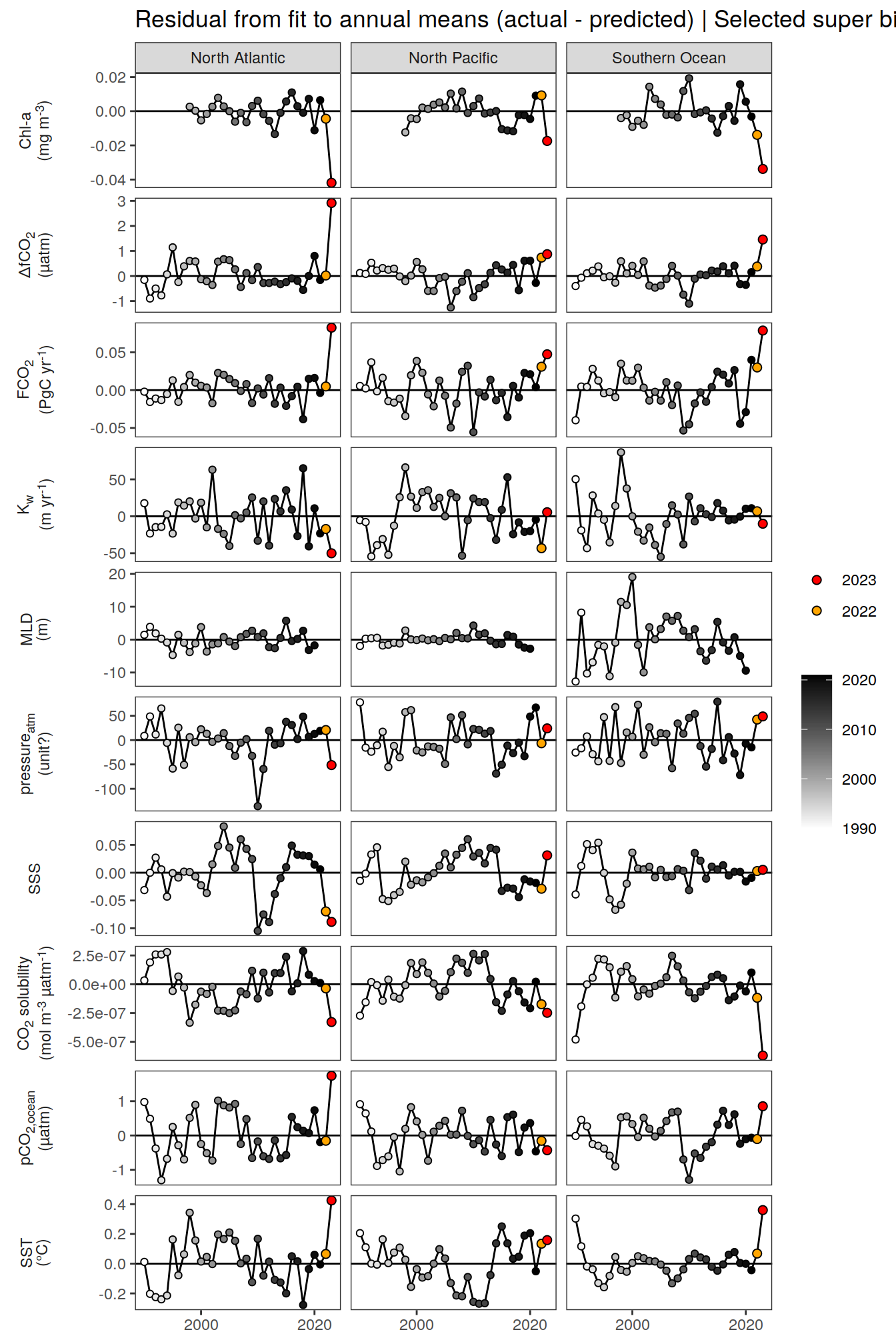
pco2_product_annual_regression %>%
  filter(biome %in% super_biomes) %>%
  ggplot(aes(year, resid)) +
  geom_hline(yintercept = 0) +
  geom_path() +
  geom_point(data = . %>% filter(year < 2022),
             aes(fill = year),
             shape = 21) +
  scale_fill_grayC() +
  new_scale_fill() +
  geom_point(data = . %>% filter(year >= 2022),
             aes(fill = as.factor(year)),
             shape = 21, size = 2)  +
  scale_fill_manual(values = c("orange", "red"),
                     guide = guide_legend(reverse = TRUE,
                                          order = 1)) +
  scale_x_continuous(breaks = seq(1980, 2020, 20)) +
  labs(title = "Residual from fit to annual means (actual - predicted) | Selected super biomes") +
  facet_grid(name ~ biome,
             scales = "free_y",
             labeller = labeller(name = x_axis_labels),
             switch = "y") +
  theme(
    strip.text.y.left = element_markdown(),
    strip.placement = "outside",
    strip.background.y = element_blank(),
    axis.title = element_blank(),
    legend.title = element_blank()
  )
| Version | Author | Date |
|---|---|---|
| e3e1491 | jens-daniel-mueller | 2024-03-21 |
pco2_product_annual_regression %>%
  filter(biome != "global") %>%
  ggplot(aes(biome, resid)) +
  geom_hline(yintercept = 0) +
  geom_jitter(data = . %>% filter(year < 2022),
             aes(fill = year),
             shape = 21, width = 0.2) +
  scale_fill_grayC() +
  new_scale_fill() +
  geom_point(data = . %>% filter(year >= 2022),
             aes(fill = as.factor(year)),
             shape = 21, size = 2)  +
  scale_fill_manual(values = c("orange", "red"),
                     guide = guide_legend(reverse = TRUE,
                                          order = 1)) +
  labs(title = "Residual from fit to annual means (actual - predicted) | All biomes") +
  facet_grid(name ~ .,
             scales = "free_y",
             labeller = labeller(name = x_axis_labels),
             switch = "y") +
  theme(
    strip.text.y.left = element_markdown(),
    strip.placement = "outside",
    strip.background.y = element_blank(),
    axis.title = element_blank(),
    legend.title = element_blank(),
        axis.text.x = element_text(angle = 90, vjust = 0.5, hjust=1)
  )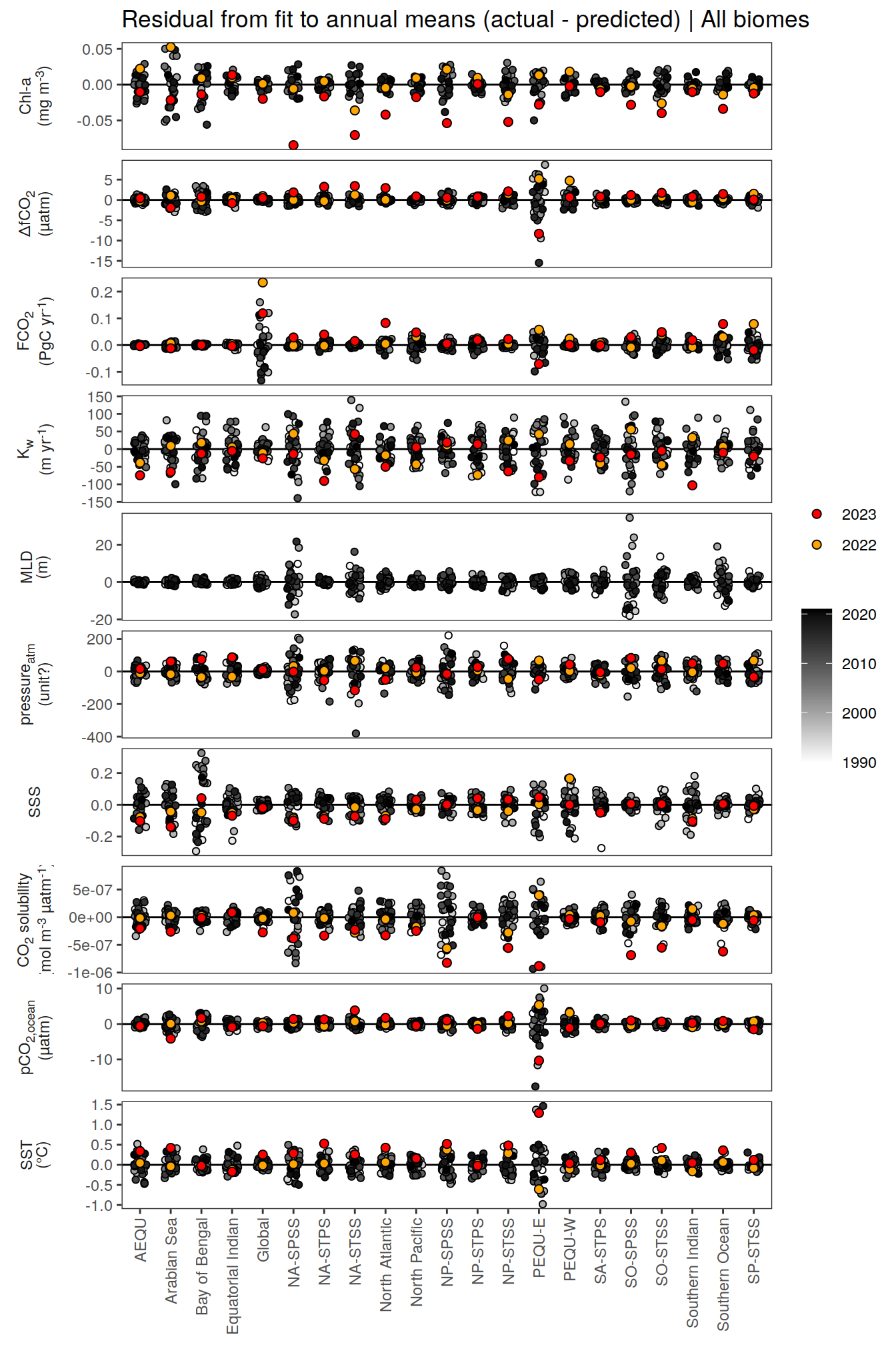
| Version | Author | Date |
|---|---|---|
| e3e1491 | jens-daniel-mueller | 2024-03-21 |
pco2_product_annual_regression %>%
  write_csv(paste0("../data/","OceanSODA","_biome_annual_regression.csv"))
pco2_product_annual_detrended <-
full_join(pco2_product_monthly,
pco2_product_annual_regression %>% select(-c(value, resid))) %>%
mutate(resid = value - fit)
pco2_product_annual_detrended %>%
filter(biome %in% "Global") %>%
ggplot(aes(month, resid, group = as.factor(year))) +
geom_path(data = . %>% filter(year < 2022),
aes(col = year)) +
scale_color_grayC() +
new_scale_color() +
geom_path(data = . %>% filter(year >= 2022),
aes(col = as.factor(year)),
linewidth = 1) +
scale_color_manual(values = c("orange", "red"),
guide = guide_legend(reverse = TRUE,
order = 1)) +
scale_x_continuous(breaks = seq(1, 12, 3), expand = c(0, 0)) +
labs(title = "Anomalies from predicted annual mean | Global") +
facet_wrap(name ~ .,
scales = "free_y",
labeller = labeller(name = x_axis_labels),
strip.position = "left",
ncol = 2) +
theme(
strip.text.y.left = element_markdown(),
strip.placement = "outside",
strip.background.y = element_blank(),
axis.title.y = element_blank(),
legend.title = element_blank()
)
| Version | Author | Date |
|---|---|---|
| 2fdbfec | jens-daniel-mueller | 2024-03-21 |
| 83fcd67 | jens-daniel-mueller | 2024-03-21 |
| 342018b | jens-daniel-mueller | 2024-03-20 |
| f0a1de7 | jens-daniel-mueller | 2024-03-20 |
| 2d2fb75 | jens-daniel-mueller | 2024-03-20 |
| d520917 | jens-daniel-mueller | 2024-03-19 |
| 03321bd | jens-daniel-mueller | 2024-03-19 |
| b41fa51 | jens-daniel-mueller | 2024-03-19 |
pco2_product_annual_detrended %>%
  filter(biome %in% key_biomes) %>%
  ggplot(aes(month, resid, group = as.factor(year))) +
  geom_path(data = . %>% filter(year < 2022),
            aes(col = year)) +
  scale_color_grayC() +
  new_scale_color() +
  geom_path(data = . %>% filter(year >= 2022),
            aes(col = as.factor(year)),
            linewidth = 1) +
  scale_color_manual(values = c("orange", "red"),
                     guide = guide_legend(reverse = TRUE,
                                          order = 1)) +
  scale_x_continuous(breaks = seq(1, 12, 3), expand = c(0, 0)) +
  labs(title = "Anomalies from predicted annual mean | Selected biomes") +
  facet_grid(name ~ biome,
             scales = "free_y",
             labeller = labeller(name = x_axis_labels),
             switch = "y") +
  theme(
    strip.text.y.left = element_markdown(),
    strip.placement = "outside",
    strip.background.y = element_blank(),
    axis.title.y = element_blank(),
    legend.title = element_blank(),
        axis.text.x = element_text(angle = 90, vjust = 0.5, hjust=1)
  )
| Version | Author | Date |
|---|---|---|
| 2fdbfec | jens-daniel-mueller | 2024-03-21 |
| 83fcd67 | jens-daniel-mueller | 2024-03-21 |
| 342018b | jens-daniel-mueller | 2024-03-20 |
| f0a1de7 | jens-daniel-mueller | 2024-03-20 |
| 2d2fb75 | jens-daniel-mueller | 2024-03-20 |
| d520917 | jens-daniel-mueller | 2024-03-19 |
| 03321bd | jens-daniel-mueller | 2024-03-19 |
| b41fa51 | jens-daniel-mueller | 2024-03-19 |
pco2_product_annual_detrended %>%
  filter(biome %in% super_biomes) %>%
  ggplot(aes(month, resid, group = as.factor(year))) +
  geom_path(data = . %>% filter(year < 2022),
            aes(col = year)) +
  scale_color_grayC() +
  new_scale_color() +
  geom_path(data = . %>% filter(year >= 2022),
            aes(col = as.factor(year)),
            linewidth = 1) +
  scale_color_manual(values = c("orange", "red"),
                     guide = guide_legend(reverse = TRUE,
                                          order = 1)) +
  scale_x_continuous(breaks = seq(1, 12, 3), expand = c(0, 0)) +
  labs(title = "Anomalies from predicted annual mean | Selected super biomes") +
  facet_grid(name ~ biome,
             scales = "free_y",
             labeller = labeller(name = x_axis_labels),
             switch = "y") +
  theme(
    strip.text.y.left = element_markdown(),
    strip.placement = "outside",
    strip.background.y = element_blank(),
    axis.title.y = element_blank(),
    legend.title = element_blank(),
        axis.text.x = element_text(angle = 90, vjust = 0.5, hjust=1)
  )
| Version | Author | Date |
|---|---|---|
| e3e1491 | jens-daniel-mueller | 2024-03-21 |
pco2_product_annual_detrended %>%
  filter(biome %in% key_biomes) %>%
  group_split(biome) %>%
  # head(1) %>%
  map(
    ~ ggplot(data = .x,
             aes(month, resid, group = as.factor(year))) +
      geom_path(data = . %>% filter(year < 2022),
                aes(col = year)) +
      scale_color_grayC() +
      new_scale_color() +
      geom_path(
        data = . %>% filter(year >= 2022),
        aes(col = as.factor(year)),
        linewidth = 1
      ) +
      scale_color_manual(
        values = c("orange", "red"),
        guide = guide_legend(reverse = TRUE,
                             order = 1)
      ) +
      scale_x_continuous(breaks = seq(1, 12, 3), expand = c(0, 0)) +
      labs(title = paste("Anomalies from predicted annual mean |", .x$biome)) +
      facet_wrap(
        name ~ .,
        scales = "free_y",
        labeller = labeller(name = x_axis_labels),
        strip.position = "left",
        ncol = 2
      ) +
      theme(
        strip.text.y.left = element_markdown(),
        strip.placement = "outside",
        strip.background.y = element_blank(),
        axis.title = element_blank(),
        legend.title = element_blank()
      )
  )
[[1]]
| Version | Author | Date |
|---|---|---|
| 2fdbfec | jens-daniel-mueller | 2024-03-21 |
| 83fcd67 | jens-daniel-mueller | 2024-03-21 |
| 342018b | jens-daniel-mueller | 2024-03-20 |
| f0a1de7 | jens-daniel-mueller | 2024-03-20 |
| 2d2fb75 | jens-daniel-mueller | 2024-03-20 |
| d520917 | jens-daniel-mueller | 2024-03-19 |
| 03321bd | jens-daniel-mueller | 2024-03-19 |
| b41fa51 | jens-daniel-mueller | 2024-03-19 |
[[2]]
| Version | Author | Date |
|---|---|---|
| 2fdbfec | jens-daniel-mueller | 2024-03-21 |
| 83fcd67 | jens-daniel-mueller | 2024-03-21 |
| 342018b | jens-daniel-mueller | 2024-03-20 |
| f0a1de7 | jens-daniel-mueller | 2024-03-20 |
| 2d2fb75 | jens-daniel-mueller | 2024-03-20 |
| d520917 | jens-daniel-mueller | 2024-03-19 |
| 03321bd | jens-daniel-mueller | 2024-03-19 |
| b41fa51 | jens-daniel-mueller | 2024-03-19 |
[[3]]
| Version | Author | Date |
|---|---|---|
| 2fdbfec | jens-daniel-mueller | 2024-03-21 |
| 83fcd67 | jens-daniel-mueller | 2024-03-21 |
| 342018b | jens-daniel-mueller | 2024-03-20 |
| f0a1de7 | jens-daniel-mueller | 2024-03-20 |
| 2d2fb75 | jens-daniel-mueller | 2024-03-20 |
| d520917 | jens-daniel-mueller | 2024-03-19 |
| 03321bd | jens-daniel-mueller | 2024-03-19 |
| b41fa51 | jens-daniel-mueller | 2024-03-19 |
[[4]]
| Version | Author | Date |
|---|---|---|
| 2fdbfec | jens-daniel-mueller | 2024-03-21 |
| 83fcd67 | jens-daniel-mueller | 2024-03-21 |
| 342018b | jens-daniel-mueller | 2024-03-20 |
| f0a1de7 | jens-daniel-mueller | 2024-03-20 |
| 2d2fb75 | jens-daniel-mueller | 2024-03-20 |
| d520917 | jens-daniel-mueller | 2024-03-19 |
| 03321bd | jens-daniel-mueller | 2024-03-19 |
| b41fa51 | jens-daniel-mueller | 2024-03-19 |
[[5]]
| Version | Author | Date |
|---|---|---|
| 2fdbfec | jens-daniel-mueller | 2024-03-21 |
| 83fcd67 | jens-daniel-mueller | 2024-03-21 |
| 342018b | jens-daniel-mueller | 2024-03-20 |
| f0a1de7 | jens-daniel-mueller | 2024-03-20 |
| 2d2fb75 | jens-daniel-mueller | 2024-03-20 |
| d520917 | jens-daniel-mueller | 2024-03-19 |
| 03321bd | jens-daniel-mueller | 2024-03-19 |
| b41fa51 | jens-daniel-mueller | 2024-03-19 |
pco2_product_annual_detrended %>%
  filter(biome %in% super_biomes) %>%
  group_split(biome) %>%
  # head(1) %>%
  map(
    ~ ggplot(data = .x,
             aes(month, resid, group = as.factor(year))) +
      geom_path(data = . %>% filter(year < 2022),
                aes(col = year)) +
      scale_color_grayC() +
      new_scale_color() +
      geom_path(
        data = . %>% filter(year >= 2022),
        aes(col = as.factor(year)),
        linewidth = 1
      ) +
      scale_color_manual(
        values = c("orange", "red"),
        guide = guide_legend(reverse = TRUE,
                             order = 1)
      ) +
      scale_x_continuous(breaks = seq(1, 12, 3), expand = c(0, 0)) +
      labs(title = paste("Anomalies from predicted annual mean |", .x$biome)) +
      facet_wrap(
        name ~ .,
        scales = "free_y",
        labeller = labeller(name = x_axis_labels),
        strip.position = "left",
        ncol = 2
      ) +
      theme(
        strip.text.y.left = element_markdown(),
        strip.placement = "outside",
        strip.background.y = element_blank(),
        axis.title = element_blank(),
        legend.title = element_blank()
      )
  )
[[1]]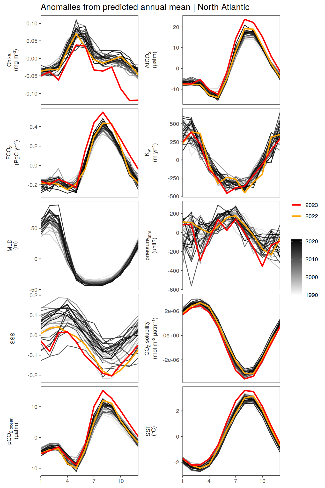
| Version | Author | Date |
|---|---|---|
| e3e1491 | jens-daniel-mueller | 2024-03-21 |
[[2]]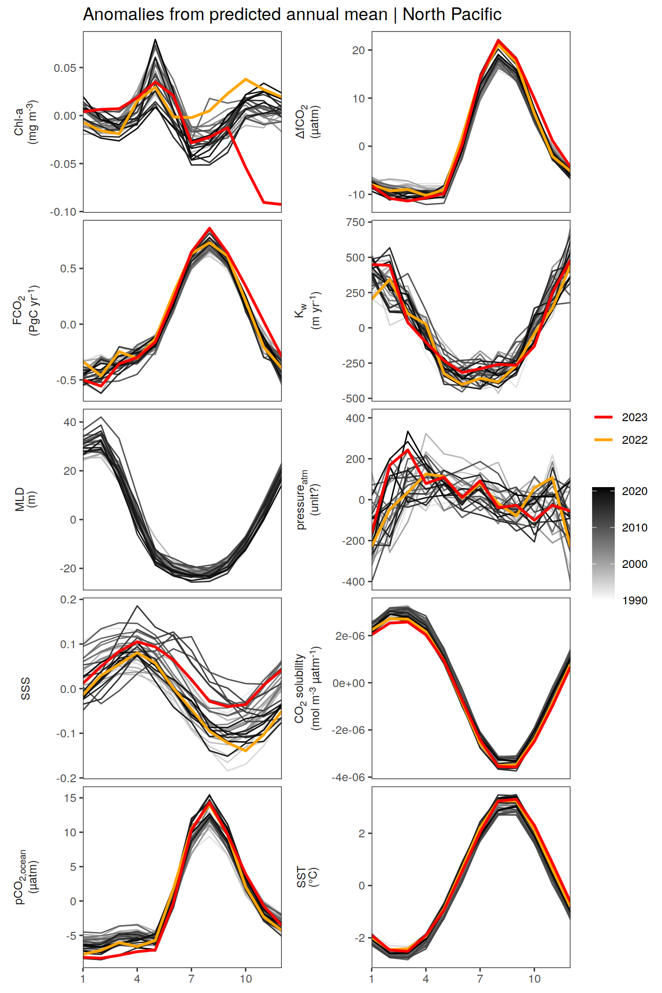
| Version | Author | Date |
|---|---|---|
| e3e1491 | jens-daniel-mueller | 2024-03-21 |
[[3]]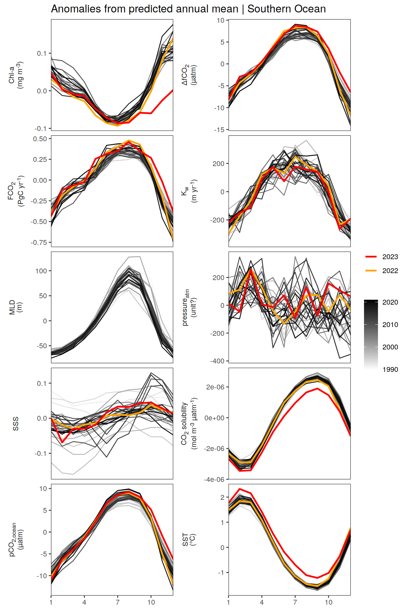
| Version | Author | Date |
|---|---|---|
| e3e1491 | jens-daniel-mueller | 2024-03-21 |
pco2_product_annual_detrended %>%
  write_csv(paste0("../data/","OceanSODA","_biome_annual_detrended.csv"))
Monthly mean trends
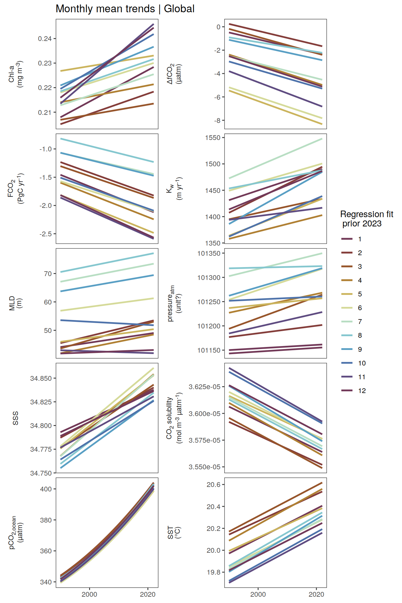
pco2_product_monthly %>%
  filter(biome %in% "Global") %>%
  mutate(month = as.factor(month)) %>%
  ggplot(aes(year, value, col = month)) +
  # geom_point() +
  geom_smooth(data = . %>% filter(year <= 2022,
                                  !(name %in% name_quadratic_fit)),
              method = "lm",
              se = FALSE,
              fullrange = TRUE) +
  geom_smooth(
    data = . %>% filter(year <= 2022,
                        name %in% name_quadratic_fit),
    method = "lm",
    fullrange = TRUE,
    formula = y ~ x + I(x ^ 2),
    se = FALSE
  ) +
  scale_color_scico_d(palette = "romaO",
    name = "Regression fit\n prior 2023") +
  scale_x_continuous(breaks = seq(1980, 2020, 20)) +
  labs(title = "Monthly mean trends | Global") +
  facet_wrap(name ~ .,
             scales = "free_y",
             labeller = labeller(name = x_axis_labels),
             strip.position = "left",
             ncol = 2) +
  theme(
    strip.text.y.left = element_markdown(),
    strip.placement = "outside",
    strip.background.y = element_blank(),
    axis.title = element_blank()
  )
| Version | Author | Date |
|---|---|---|
| 2fdbfec | jens-daniel-mueller | 2024-03-21 |
| 83fcd67 | jens-daniel-mueller | 2024-03-21 |
| 342018b | jens-daniel-mueller | 2024-03-20 |
| f0a1de7 | jens-daniel-mueller | 2024-03-20 |
| 2d2fb75 | jens-daniel-mueller | 2024-03-20 |
| d520917 | jens-daniel-mueller | 2024-03-19 |
| 03321bd | jens-daniel-mueller | 2024-03-19 |
| b41fa51 | jens-daniel-mueller | 2024-03-19 |
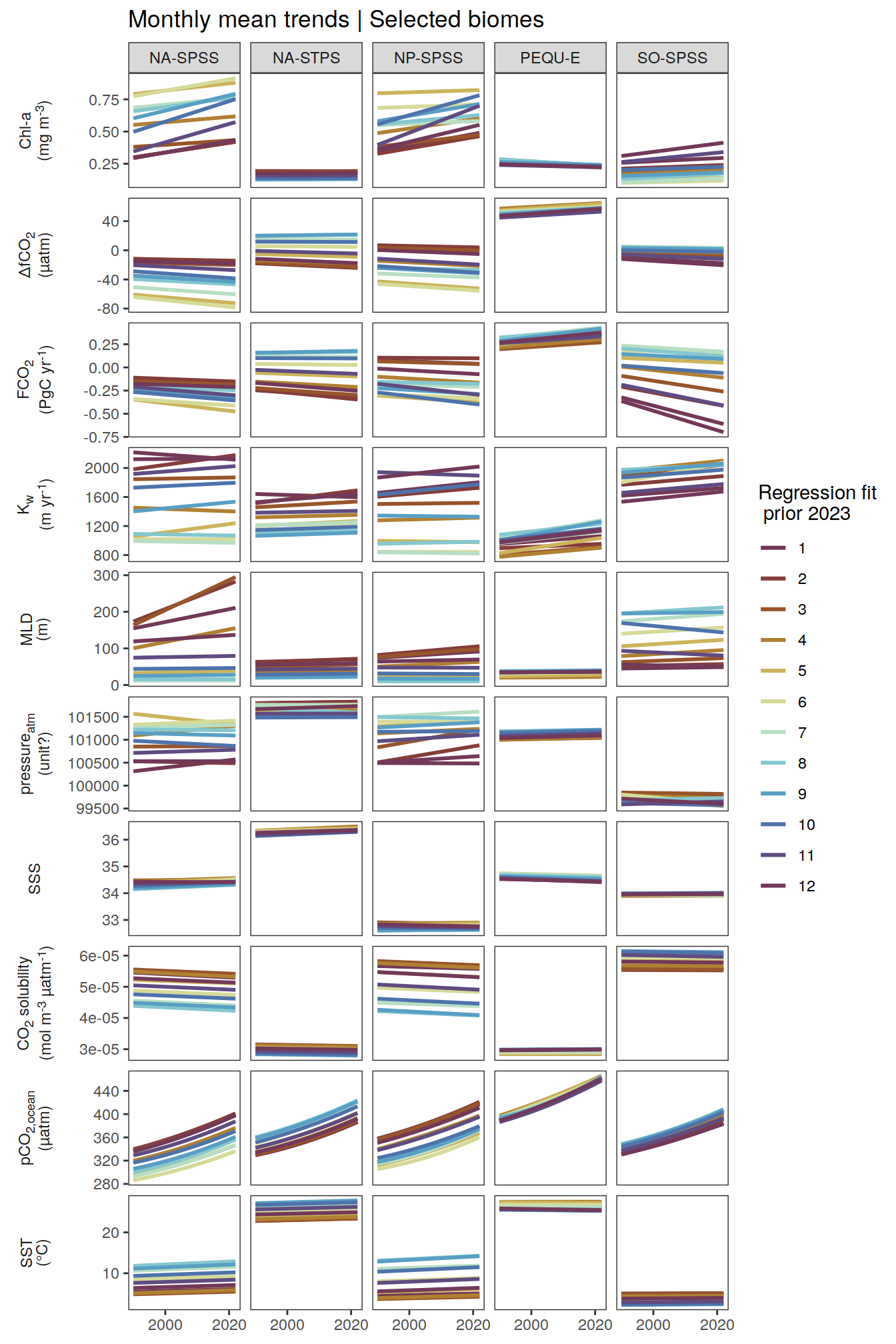
pco2_product_monthly %>%
  filter(biome %in% key_biomes) %>%
  mutate(month = as.factor(month)) %>%
  ggplot(aes(year, value, col = month)) +
  # geom_point() +
  geom_smooth(data = . %>% filter(year <= 2022,
                                  !(name %in% name_quadratic_fit)),
              method = "lm",
              fullrange = TRUE,
              se = FALSE) +
  geom_smooth(
    data = . %>% filter(year <= 2022,
                        name %in% name_quadratic_fit),
    method = "lm",
    fullrange = TRUE,
    formula = y ~ x + I(x ^ 2),
    se = FALSE
  ) +
  scale_color_scico_d(palette = "romaO",
    name = "Regression fit\n prior 2023") +
  scale_x_continuous(breaks = seq(1980, 2020, 20)) +
  labs(title = "Monthly mean trends | Selected biomes") +
  facet_grid(name ~ biome,
             scales = "free_y",
             labeller = labeller(name = x_axis_labels),
             switch = "y") +
  theme(
    strip.text.y.left = element_markdown(),
    strip.placement = "outside",
    strip.background.y = element_blank(),
    axis.title = element_blank()
  )
| Version | Author | Date |
|---|---|---|
| 2fdbfec | jens-daniel-mueller | 2024-03-21 |
| 83fcd67 | jens-daniel-mueller | 2024-03-21 |
| 342018b | jens-daniel-mueller | 2024-03-20 |
| f0a1de7 | jens-daniel-mueller | 2024-03-20 |
| 2d2fb75 | jens-daniel-mueller | 2024-03-20 |
| d520917 | jens-daniel-mueller | 2024-03-19 |
| 03321bd | jens-daniel-mueller | 2024-03-19 |
| b41fa51 | jens-daniel-mueller | 2024-03-19 |
pco2_product_monthly_regression <-
  pco2_product_monthly %>%
  anomaly_determination(biome, month)


pco2_product_monthly_regression %>%
  filter(biome %in% "Global") %>%
  group_split(month) %>%
  head(1) %>%
  map(
    ~ ggplot(data = .x,
             aes(year, resid)) +
      geom_hline(yintercept = 0) +
      geom_path() +
      geom_point(
        data = . %>% filter(year < 2022),
        aes(fill = year),
        shape = 21
      ) +
      scale_fill_grayC() +
      new_scale_fill() +
      geom_point(
        data = . %>% filter(year >= 2022),
        aes(fill = as.factor(year)),
        shape = 21,
        size = 2
      )  +
      scale_fill_manual(
        values = c("orange", "red"),
        guide = guide_legend(reverse = TRUE,
                             order = 1)
      ) +
      scale_x_continuous(breaks = seq(1980, 2020, 20)) +
      labs(title = "Residual from fit to monthly means (actual - predicted) | Global",
           subtitle = paste("Month:", .x$month)) +
      facet_wrap(
        name ~ .,
        scales = "free_y",
        labeller = labeller(name = x_axis_labels),
        strip.position = "left",
        ncol = 2
      ) +
      theme(
        strip.text.y.left = element_markdown(),
        strip.placement = "outside",
        strip.background.y = element_blank(),
        axis.title = element_blank(),
        legend.title = element_blank()
      )
  )
[[1]]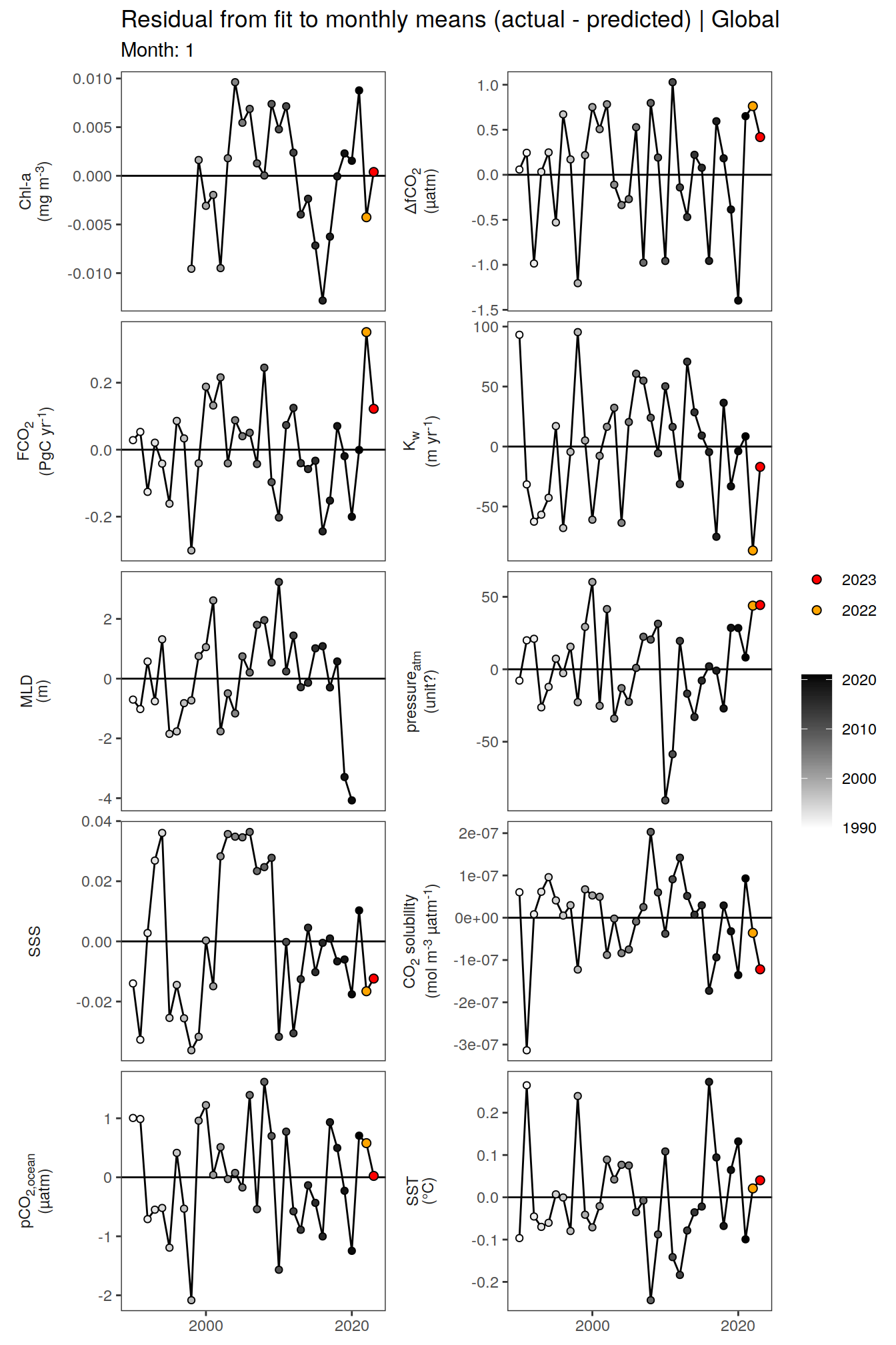
| Version | Author | Date |
|---|---|---|
| 2fdbfec | jens-daniel-mueller | 2024-03-21 |
| 83fcd67 | jens-daniel-mueller | 2024-03-21 |
| 342018b | jens-daniel-mueller | 2024-03-20 |
| f0a1de7 | jens-daniel-mueller | 2024-03-20 |
| 2d2fb75 | jens-daniel-mueller | 2024-03-20 |
| d520917 | jens-daniel-mueller | 2024-03-19 |
| 03321bd | jens-daniel-mueller | 2024-03-19 |
| b41fa51 | jens-daniel-mueller | 2024-03-19 |
pco2_product_monthly_regression %>%
  filter(biome %in% key_biomes) %>%
  group_split(month) %>%
  head(1) %>%
  map(
    ~ ggplot(data = .x,
             aes(year, resid)) +
      geom_hline(yintercept = 0) +
      geom_path() +
      geom_point(
        data = . %>% filter(year < 2022),
        aes(fill = year),
        shape = 21
      ) +
      scale_fill_grayC() +
      new_scale_fill() +
      geom_point(
        data = . %>% filter(year >= 2022),
        aes(fill = as.factor(year)),
        shape = 21,
        size = 2
      )  +
      scale_fill_manual(
        values = c("orange", "red"),
        guide = guide_legend(reverse = TRUE,
                             order = 1)
      ) +
      scale_x_continuous(breaks = seq(1980, 2020, 20)) +
      labs(title = "Residual from fit to monthly means (actual - predicted) | Selected biomes",
           subtitle = paste("Month:", .x$month)) +
      facet_grid(
        name ~ biome,
        scales = "free_y",
        labeller = labeller(name = x_axis_labels),
        switch = "y"
      ) +
      theme(
        strip.text.y.left = element_markdown(),
        strip.placement = "outside",
        strip.background.y = element_blank(),
        axis.title = element_blank(),
        legend.title = element_blank()
      )
  )
[[1]]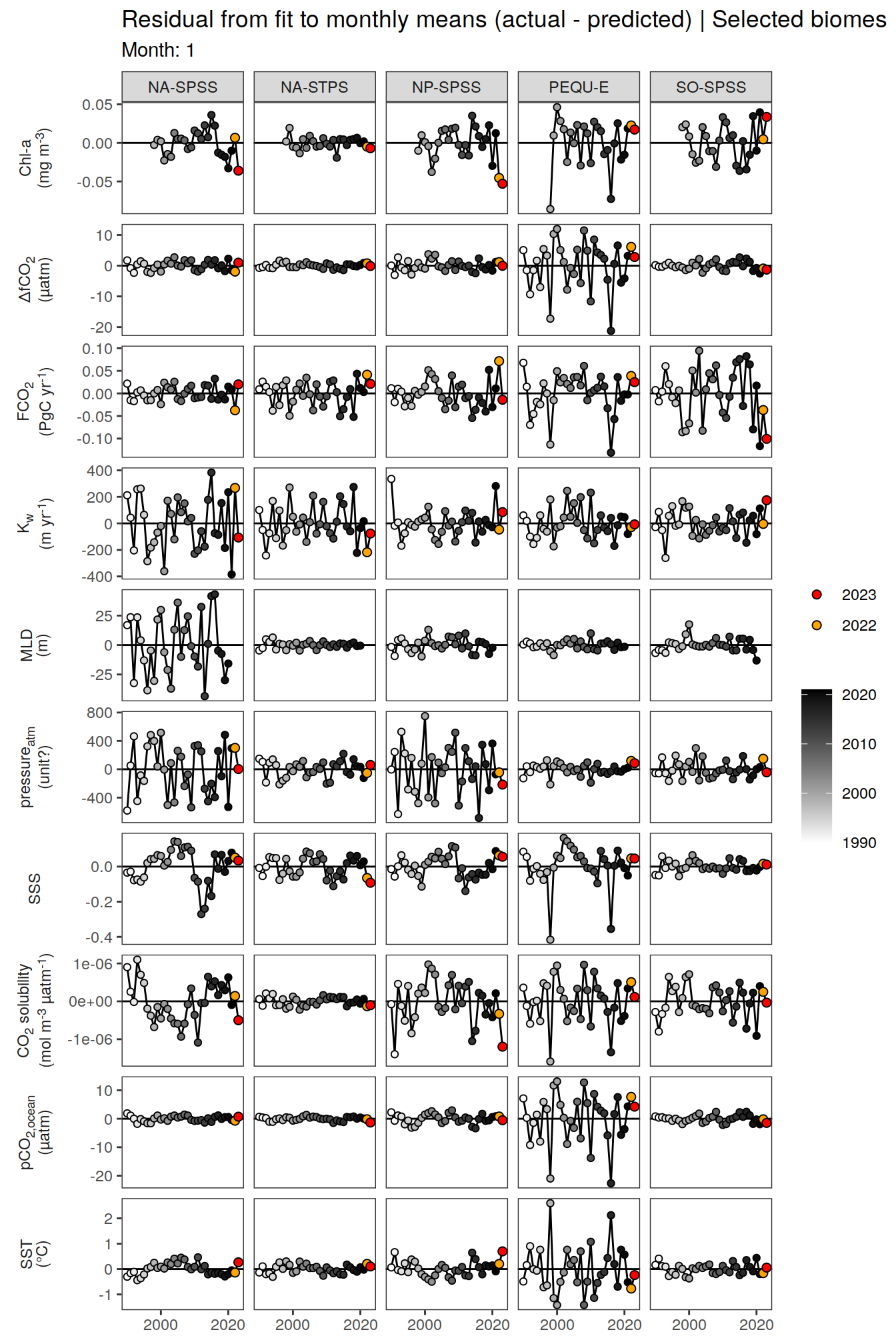
| Version | Author | Date |
|---|---|---|
| e3e1491 | jens-daniel-mueller | 2024-03-21 |
| 2fdbfec | jens-daniel-mueller | 2024-03-21 |
| 83fcd67 | jens-daniel-mueller | 2024-03-21 |
| 342018b | jens-daniel-mueller | 2024-03-20 |
| f0a1de7 | jens-daniel-mueller | 2024-03-20 |
| 2d2fb75 | jens-daniel-mueller | 2024-03-20 |
| d520917 | jens-daniel-mueller | 2024-03-19 |
| 03321bd | jens-daniel-mueller | 2024-03-19 |
| b41fa51 | jens-daniel-mueller | 2024-03-19 |
pco2_product_monthly_detrended <-
  full_join(pco2_product_monthly,
            pco2_product_monthly_regression %>% select(-c(value, resid, time))) %>%
  mutate(resid = value - fit)

pco2_product_monthly_detrended %>%
  filter(biome %in% "Global") %>%
  ggplot(aes(month, resid, group = as.factor(year))) +
  geom_path(data = . %>% filter(year < 2022),
            aes(col = year)) +
  scale_color_grayC() +
  new_scale_color() +
  geom_path(data = . %>% filter(year >= 2022),
            aes(col = as.factor(year)),
            linewidth = 1) +
  scale_color_manual(values = c("orange", "red"),
                     guide = guide_legend(reverse = TRUE,
                                          order = 1)) +
  scale_x_continuous(breaks = seq(1, 12, 3), expand = c(0, 0)) +
  labs(title = "Anomalies from predicted monthly mean | Global") +
  facet_wrap(
    name ~ .,
    scales = "free_y",
    labeller = labeller(name = x_axis_labels),
    strip.position = "left",
    ncol = 2
  ) +
  theme(
    strip.text.y.left = element_markdown(),
    strip.placement = "outside",
    strip.background.y = element_blank(),
    axis.title.y = element_blank(),
    legend.title = element_blank()
  )
| Version | Author | Date |
|---|---|---|
| 2fdbfec | jens-daniel-mueller | 2024-03-21 |
| 83fcd67 | jens-daniel-mueller | 2024-03-21 |
| 342018b | jens-daniel-mueller | 2024-03-20 |
| f0a1de7 | jens-daniel-mueller | 2024-03-20 |
| 2d2fb75 | jens-daniel-mueller | 2024-03-20 |
| d520917 | jens-daniel-mueller | 2024-03-19 |
| 03321bd | jens-daniel-mueller | 2024-03-19 |
| b41fa51 | jens-daniel-mueller | 2024-03-19 |
pco2_product_monthly_detrended %>%
  filter(biome %in% key_biomes) %>%
  ggplot(aes(month, resid, group = as.factor(year))) +
  geom_path(data = . %>% filter(year < 2022),
            aes(col = year)) +
  scale_color_grayC() +
  new_scale_color() +
  geom_path(data = . %>% filter(year >= 2022),
            aes(col = as.factor(year)),
            linewidth = 1) +
  scale_color_manual(values = c("orange", "red"),
                     guide = guide_legend(reverse = TRUE,
                                          order = 1)) +
  scale_x_continuous(breaks = seq(1, 12, 3), expand = c(0, 0)) +
  labs(title = "Anomalies from predicted monthly mean | Selected biomes") +
  facet_grid(
    name ~ biome,
    scales = "free_y",
    labeller = labeller(name = x_axis_labels),
    switch = "y"
  ) +
  theme(
    strip.text.y.left = element_markdown(),
    strip.placement = "outside",
    strip.background.y = element_blank(),
    axis.title.y = element_blank(),
    legend.title = element_blank()
  )
| Version | Author | Date |
|---|---|---|
| 2fdbfec | jens-daniel-mueller | 2024-03-21 |
| 83fcd67 | jens-daniel-mueller | 2024-03-21 |
| 342018b | jens-daniel-mueller | 2024-03-20 |
| f0a1de7 | jens-daniel-mueller | 2024-03-20 |
| 2d2fb75 | jens-daniel-mueller | 2024-03-20 |
| d520917 | jens-daniel-mueller | 2024-03-19 |
| 03321bd | jens-daniel-mueller | 2024-03-19 |
| b41fa51 | jens-daniel-mueller | 2024-03-19 |
pco2_product_monthly_detrended %>%
  filter(biome %in% super_biomes) %>%
  ggplot(aes(month, resid, group = as.factor(year))) +
  geom_path(data = . %>% filter(year < 2022),
            aes(col = year)) +
  scale_color_grayC() +
  new_scale_color() +
  geom_path(data = . %>% filter(year >= 2022),
            aes(col = as.factor(year)),
            linewidth = 1) +
  scale_color_manual(values = c("orange", "red"),
                     guide = guide_legend(reverse = TRUE,
                                          order = 1)) +
  scale_x_continuous(breaks = seq(1, 12, 3), expand = c(0, 0)) +
  labs(title = "Anomalies from predicted monthly mean | Selected super biomes") +
  facet_grid(
    name ~ biome,
    scales = "free_y",
    labeller = labeller(name = x_axis_labels),
    switch = "y"
  ) +
  theme(
    strip.text.y.left = element_markdown(),
    strip.placement = "outside",
    strip.background.y = element_blank(),
    axis.title.y = element_blank(),
    legend.title = element_blank()
  )
| Version | Author | Date |
|---|---|---|
| e3e1491 | jens-daniel-mueller | 2024-03-21 |
pco2_product_monthly_detrended %>%
  filter(biome %in% key_biomes) %>%
  group_split(biome) %>%
  # head(1) %>%
  map(
    ~ ggplot(data = .x,
             aes(month, resid, group = as.factor(year))) +
      geom_path(data = . %>% filter(year < 2022),
                aes(col = year)) +
      scale_color_grayC() +
      new_scale_color() +
      geom_path(
        data = . %>% filter(year >= 2022),
        aes(col = as.factor(year)),
        linewidth = 1
      ) +
      scale_color_manual(
        values = c("orange", "red"),
        guide = guide_legend(reverse = TRUE,
                             order = 1)
      ) +
      scale_x_continuous(breaks = seq(1, 12, 3), expand = c(0, 0)) +
      labs(title = paste("Anomalies from predicted monthly mean |", .x$biome)) +
      facet_wrap(
        name ~ .,
        scales = "free_y",
        labeller = labeller(name = x_axis_labels),
        strip.position = "left",
        ncol = 2
      ) +
      theme(
        strip.text.y.left = element_markdown(),
        strip.placement = "outside",
        strip.background.y = element_blank(),
        axis.title.y = element_blank(),
        legend.title = element_blank()
      )
  )
[[1]]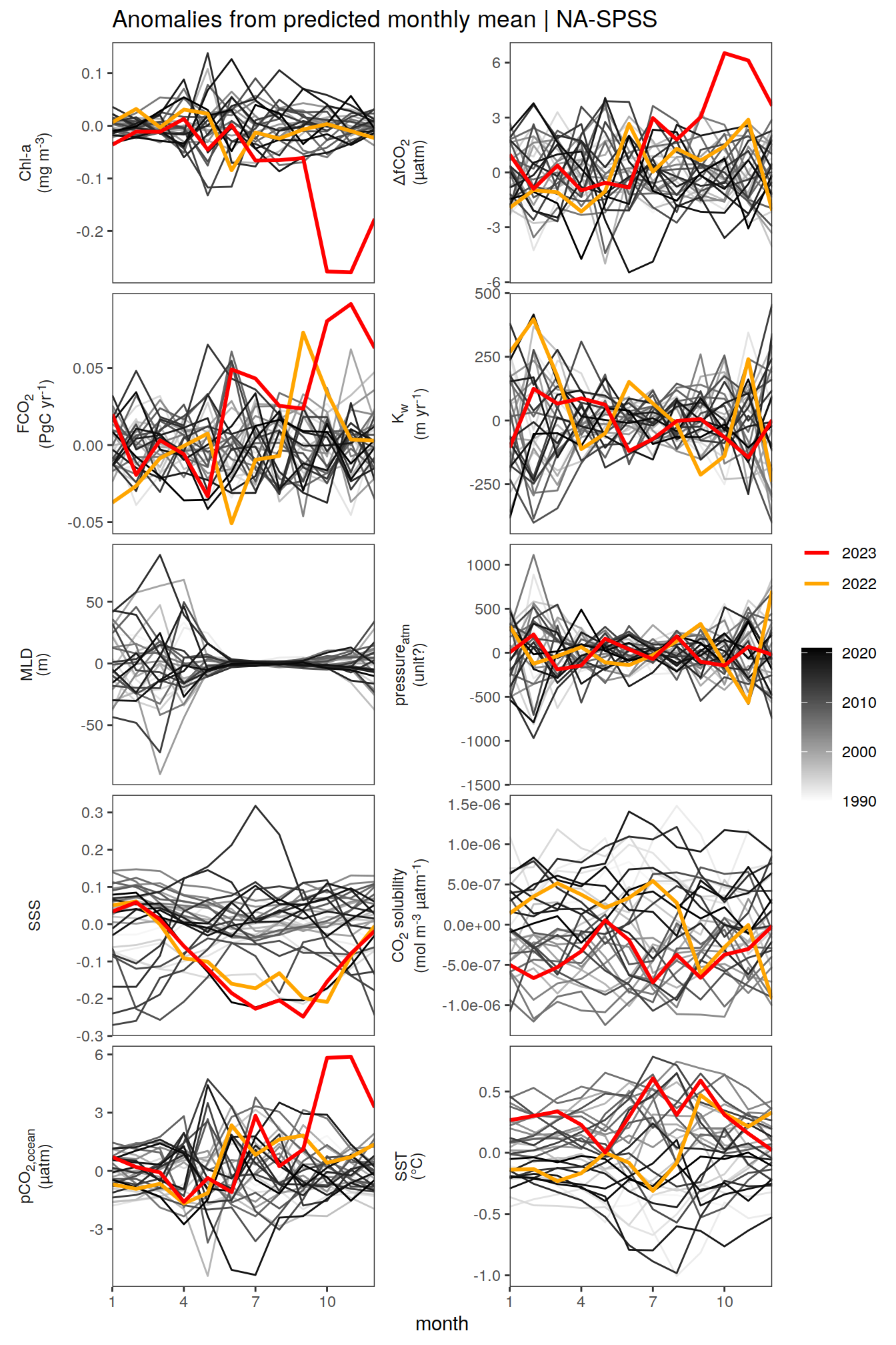
| Version | Author | Date |
|---|---|---|
| 2fdbfec | jens-daniel-mueller | 2024-03-21 |
| 83fcd67 | jens-daniel-mueller | 2024-03-21 |
| 342018b | jens-daniel-mueller | 2024-03-20 |
| f0a1de7 | jens-daniel-mueller | 2024-03-20 |
| 2d2fb75 | jens-daniel-mueller | 2024-03-20 |
| d520917 | jens-daniel-mueller | 2024-03-19 |
| 03321bd | jens-daniel-mueller | 2024-03-19 |
| b41fa51 | jens-daniel-mueller | 2024-03-19 |
[[2]]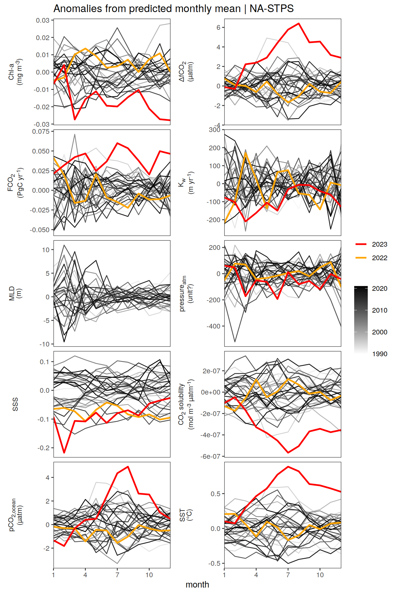
| Version | Author | Date |
|---|---|---|
| 2fdbfec | jens-daniel-mueller | 2024-03-21 |
| 83fcd67 | jens-daniel-mueller | 2024-03-21 |
| 342018b | jens-daniel-mueller | 2024-03-20 |
| f0a1de7 | jens-daniel-mueller | 2024-03-20 |
| 2d2fb75 | jens-daniel-mueller | 2024-03-20 |
| d520917 | jens-daniel-mueller | 2024-03-19 |
| 03321bd | jens-daniel-mueller | 2024-03-19 |
| b41fa51 | jens-daniel-mueller | 2024-03-19 |
[[3]]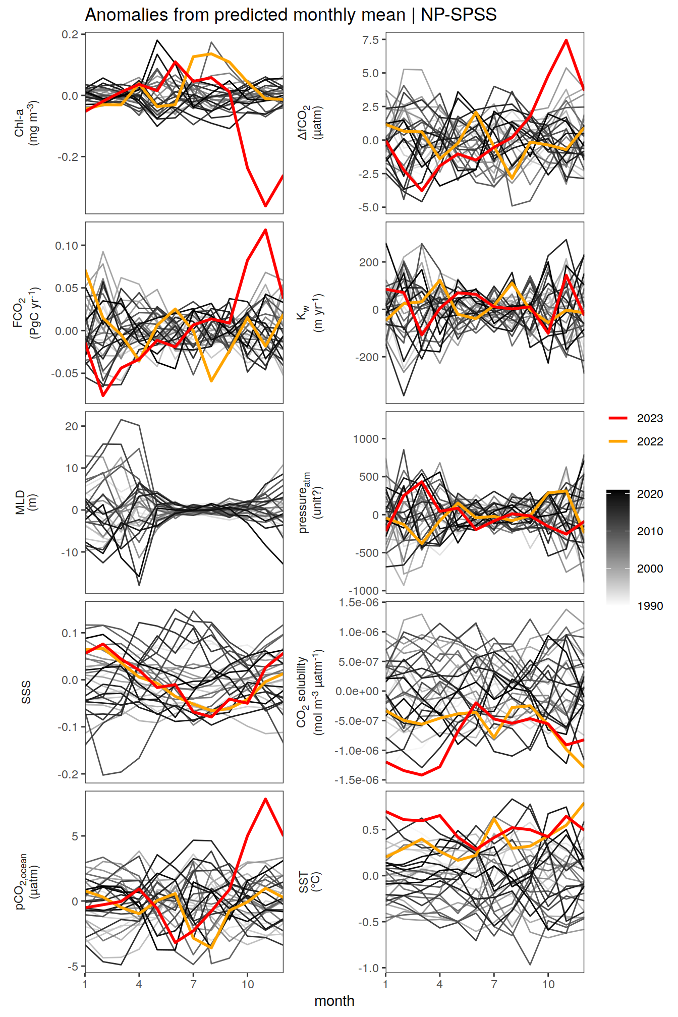
| Version | Author | Date |
|---|---|---|
| 2fdbfec | jens-daniel-mueller | 2024-03-21 |
| 83fcd67 | jens-daniel-mueller | 2024-03-21 |
| 342018b | jens-daniel-mueller | 2024-03-20 |
| f0a1de7 | jens-daniel-mueller | 2024-03-20 |
| 2d2fb75 | jens-daniel-mueller | 2024-03-20 |
| d520917 | jens-daniel-mueller | 2024-03-19 |
| 03321bd | jens-daniel-mueller | 2024-03-19 |
| b41fa51 | jens-daniel-mueller | 2024-03-19 |
[[4]]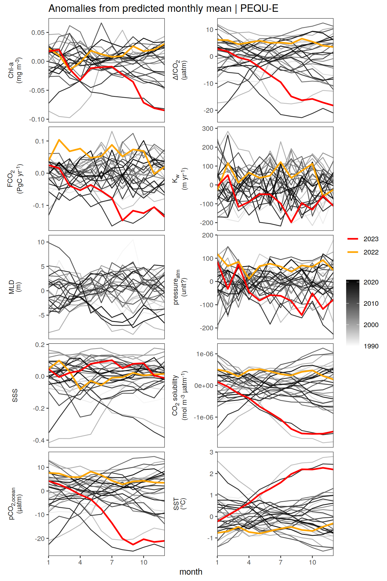
| Version | Author | Date |
|---|---|---|
| 2fdbfec | jens-daniel-mueller | 2024-03-21 |
| 83fcd67 | jens-daniel-mueller | 2024-03-21 |
| 342018b | jens-daniel-mueller | 2024-03-20 |
| f0a1de7 | jens-daniel-mueller | 2024-03-20 |
| 2d2fb75 | jens-daniel-mueller | 2024-03-20 |
| d520917 | jens-daniel-mueller | 2024-03-19 |
| 03321bd | jens-daniel-mueller | 2024-03-19 |
| b41fa51 | jens-daniel-mueller | 2024-03-19 |
[[5]]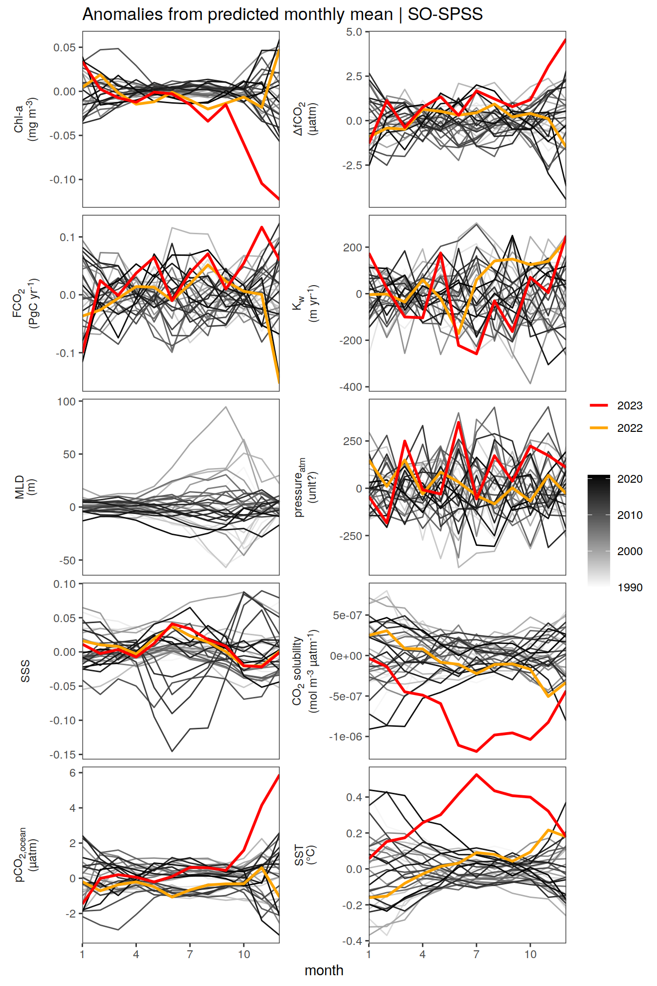
| Version | Author | Date |
|---|---|---|
| 2fdbfec | jens-daniel-mueller | 2024-03-21 |
| 83fcd67 | jens-daniel-mueller | 2024-03-21 |
| 342018b | jens-daniel-mueller | 2024-03-20 |
| f0a1de7 | jens-daniel-mueller | 2024-03-20 |
| 2d2fb75 | jens-daniel-mueller | 2024-03-20 |
| d520917 | jens-daniel-mueller | 2024-03-19 |
| 03321bd | jens-daniel-mueller | 2024-03-19 |
| b41fa51 | jens-daniel-mueller | 2024-03-19 |
pco2_product_monthly_detrended %>%
  filter(biome %in% super_biomes) %>%
  group_split(biome) %>%
  # head(1) %>%
  map(
    ~ ggplot(data = .x,
             aes(month, resid, group = as.factor(year))) +
      geom_path(data = . %>% filter(year < 2022),
                aes(col = year)) +
      scale_color_grayC() +
      new_scale_color() +
      geom_path(
        data = . %>% filter(year >= 2022),
        aes(col = as.factor(year)),
        linewidth = 1
      ) +
      scale_color_manual(
        values = c("orange", "red"),
        guide = guide_legend(reverse = TRUE,
                             order = 1)
      ) +
      scale_x_continuous(breaks = seq(1, 12, 3), expand = c(0, 0)) +
      labs(title = paste("Anomalies from predicted monthly mean |", .x$biome)) +
      facet_wrap(
        name ~ .,
        scales = "free_y",
        labeller = labeller(name = x_axis_labels),
        strip.position = "left",
        ncol = 2
      ) +
      theme(
        strip.text.y.left = element_markdown(),
        strip.placement = "outside",
        strip.background.y = element_blank(),
        axis.title.y = element_blank(),
        legend.title = element_blank()
      )
  )
[[1]]
| Version | Author | Date |
|---|---|---|
| e3e1491 | jens-daniel-mueller | 2024-03-21 |
[[2]]
| Version | Author | Date |
|---|---|---|
| e3e1491 | jens-daniel-mueller | 2024-03-21 |
[[3]]
| Version | Author | Date |
|---|---|---|
| e3e1491 | jens-daniel-mueller | 2024-03-21 |
Flux anomaly correlation
The following plots aim to unravel the correlation between biome- or globally- integrated monthly flux anomalies and the corresponding anomalies of the means/integrals of each other variable.
Anomalies are first presented are first presented in absolute units. Due to the different flux magnitudes, we need to plot the globally and biome-integrated fluxes separately. Secondly, we normalize the anomalies to the monthly spread (expressed as standard deviation) of the anomalies from 1990 to 2022.
Annual anomalies
Absolute
pco2_product_annual_regression %>%
  filter(biome == "Global") %>%
  select(-c(value, fit)) %>%
  pivot_wider(values_from = resid) %>%
  pivot_longer(-c(year, biome, fgco2_int))  %>%
  ggplot(aes(value, fgco2_int)) +
  geom_hline(yintercept = 0) +
  geom_point(data = . %>% filter(year <= 2022),
             aes(fill = year),
             shape = 21) +
  geom_smooth(
    data = . %>% filter(year <= 2022),
    method = "lm",
    se = FALSE,
    fullrange = TRUE,
    aes(col = "Regression fit\n prior 2023")
  ) +
  scale_color_grey() +
  scale_fill_grayC()+
  new_scale_fill() +
  geom_point(data = . %>% filter(year >= 2022),
             aes(fill = as.factor(year)),
             shape = 21, size = 2)  +
  scale_fill_manual(values = c("orange", "red"),
                     guide = guide_legend(reverse = TRUE,
                                          order = 1)) +
  labs(title = "Globally integrated fluxes",
       y = labels_breaks("fgco2_int")$i_legend_title) +
  facet_wrap(
    ~ name,
    scales = "free_x",
    labeller = labeller(name = x_axis_labels),
    strip.position = "bottom",
    ncol = 2
  ) +
  theme(
    strip.text.x.bottom = element_markdown(),
    strip.placement = "outside",
    strip.background.x = element_blank(),
    axis.title.y = element_markdown(),
    axis.title.x = element_blank(),
    legend.title = element_blank()
  )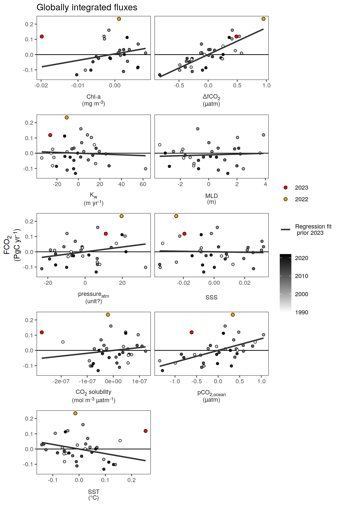
Monthly anomalies
Absolute
pco2_product_monthly_detrended_anomaly <-
  pco2_product_monthly_detrended %>%
  select(year, month, biome, name, resid) %>%
  pivot_wider(names_from = name,
              values_from = resid)


pco2_product_monthly_detrended_anomaly %>%
  filter(biome == "Global") %>%
  pivot_longer(-c(year, month, biome, fgco2_int))  %>%
  ggplot(aes(value, fgco2_int)) +
  geom_hline(yintercept = 0) +
  geom_point(data = . %>% filter(year <= 2022),
             aes(col = paste(min(year), max(year), sep = "-")),
             alpha = 0.2) +
  geom_smooth(
    data = . %>% filter(year <= 2022),
    aes(col = paste(min(year), max(year), sep = "-")),
    method = "lm",
    se = FALSE,
    fullrange = TRUE
  )  +
  scale_color_grey(name = "") +
  new_scale_color() +
  # geom_smooth(data = . %>% filter(year <= 2022),
  #             method = "lm", se = FALSE,
  #           aes(col = as.factor(month)))  +
  geom_path(data = . %>% filter(year > 2022),
            aes(col = as.factor(month), group = 1))  +
  geom_point(data = . %>% filter(year > 2022),
             aes(fill =  as.factor(month)),
             shape = 21,
             size = 3)  +
  scale_color_scico_d(palette = "buda",
                     guide = guide_legend(reverse = TRUE,
                                          order = 1),
                     name = "Month\nof 2023") +
  scale_fill_scico_d(palette = "buda",
                     guide = guide_legend(reverse = TRUE,
                                          order = 1),
                     name = "Month\nof 2023") +
  labs(title = "Globally integrated fluxes",
       y = labels_breaks("fgco2_int")$i_legend_title) +
  facet_wrap(
    ~ name,
    scales = "free_x",
    labeller = labeller(name = x_axis_labels),
    strip.position = "bottom",
    ncol = 2
  ) +
  theme(
    strip.text.x.bottom = element_markdown(),
    strip.placement = "outside",
    strip.background.x = element_blank(),
    axis.title.y = element_markdown(),
    axis.title.x = element_blank()
  )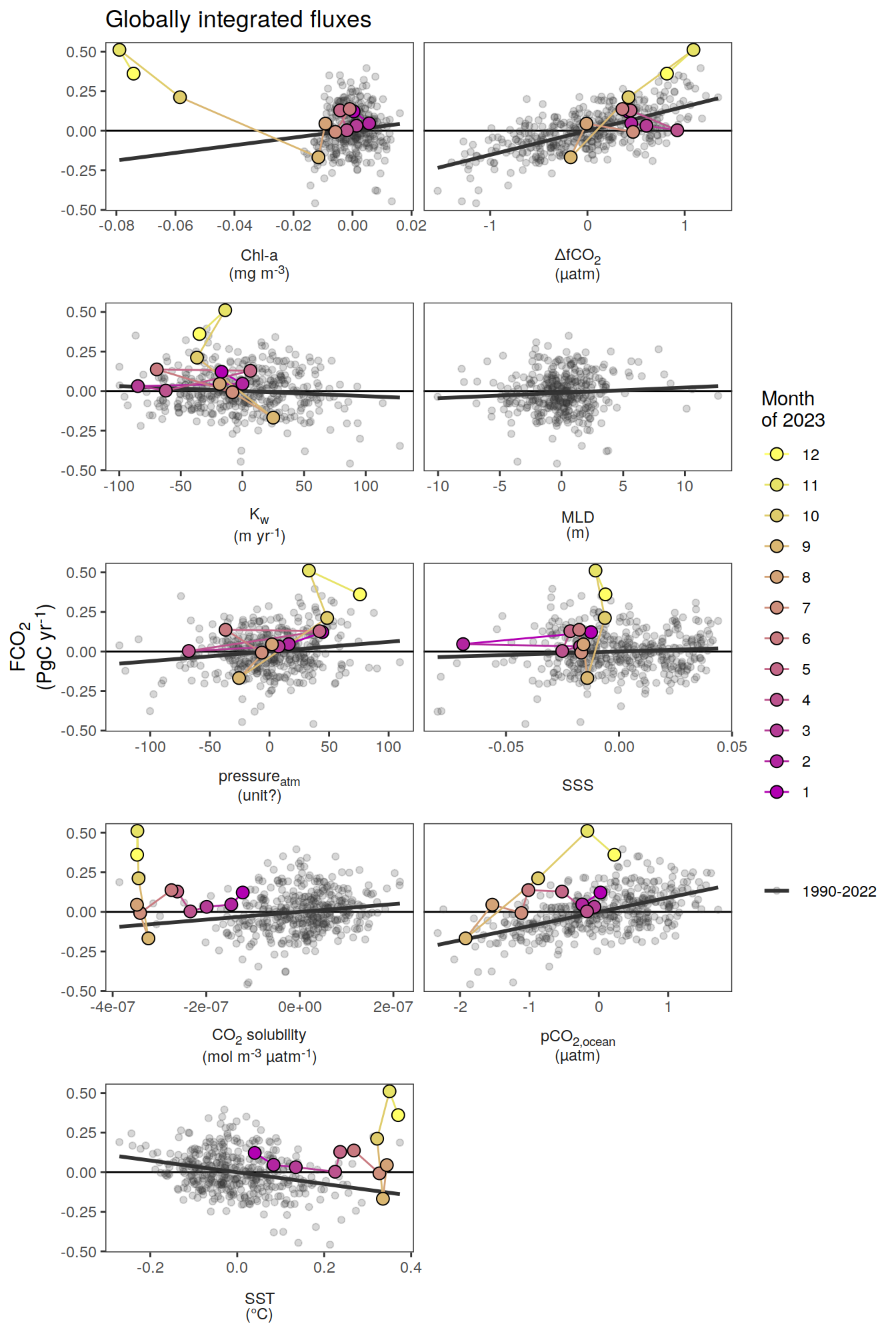
pco2_product_monthly_detrended_anomaly %>%
  filter(!(biome %in% c(super_biomes, "Global"))) %>%
  pivot_longer(-c(year, month, biome, fgco2_int))  %>%
  group_split(name) %>%
  # head(1) %>%
  map(
    ~ ggplot(data = .x,
             aes(value, fgco2_int)) +
      geom_hline(yintercept = 0) +
      geom_point(
        data = . %>% filter(year <= 2022),
        aes(col = paste(min(year), max(year), sep = "-")),
        alpha = 0.2
      ) +
      geom_smooth(
        data = . %>% filter(year <= 2022),
        aes(col = paste(min(year), max(year), sep = "-")),
        method = "lm",
        se = FALSE,
        fullrange = TRUE
      )  +
      scale_color_grey(name = "") +
      new_scale_color() +
      geom_path(data = . %>% filter(year > 2022),
                aes(col = as.factor(month), group = 1))  +
      geom_point(
        data = . %>% filter(year > 2022),
        aes(fill = as.factor(month)),
        shape = 21,
        size = 3
      )  +
      scale_color_scico_d(
        palette = "buda",
        guide = guide_legend(reverse = TRUE,
                             order = 1),
        name = "Month\nof 2023"
      ) +
      scale_fill_scico_d(
        palette = "buda",
        guide = guide_legend(reverse = TRUE,
                             order = 1),
        name = "Month\nof 2023"
      ) +
      facet_wrap( ~ biome, ncol = 3, scales = "free_x") +
      labs(
        title = "Biome integrated fluxes",
        y = labels_breaks("fgco2_int")$i_legend_title,
        x = labels_breaks(.x %>% distinct(name))$i_legend_title
      ) +
      theme(axis.title.x = element_markdown(),
            axis.title.y = element_markdown())
  )
[[1]]
[[2]]
[[3]]
[[4]]
[[5]]
[[6]]
[[7]]
[[8]]
[[9]]
pco2_product_monthly_detrended_anomaly %>%
  filter(biome %in% super_biomes) %>%
  pivot_longer(-c(year, month, biome, fgco2_int))  %>%
  group_split(name) %>%
  # head(1) %>%
  map(
    ~ ggplot(data = .x,
             aes(value, fgco2_int)) +
      geom_hline(yintercept = 0) +
      geom_point(
        data = . %>% filter(year <= 2022),
        aes(col = paste(min(year), max(year), sep = "-")),
        alpha = 0.2
      ) +
      geom_smooth(
        data = . %>% filter(year <= 2022),
        aes(col = paste(min(year), max(year), sep = "-")),
        method = "lm",
        se = FALSE,
        fullrange = TRUE
      )  +
      scale_color_grey(name = "") +
      new_scale_color() +
      geom_path(data = . %>% filter(year > 2022),
                aes(col = as.factor(month), group = 1))  +
      geom_point(
        data = . %>% filter(year > 2022),
        aes(fill = as.factor(month)),
        shape = 21,
        size = 3
      )  +
      scale_color_scico_d(
        palette = "buda",
        guide = guide_legend(reverse = TRUE,
                             order = 1),
        name = "Month\nof 2023"
      ) +
      scale_fill_scico_d(
        palette = "buda",
        guide = guide_legend(reverse = TRUE,
                             order = 1),
        name = "Month\nof 2023"
      ) +
      facet_wrap( ~ biome, ncol = 3, scales = "free_x") +
      labs(
        title = "Super biome integrated fluxes",
        y = labels_breaks("fgco2_int")$i_legend_title,
        x = labels_breaks(.x %>% distinct(name))$i_legend_title
      ) +
      theme(axis.title.x = element_markdown(),
            axis.title.y = element_markdown())
  )
[[1]]
| Version | Author | Date |
|---|---|---|
| e3e1491 | jens-daniel-mueller | 2024-03-21 |
[[2]]
| Version | Author | Date |
|---|---|---|
| e3e1491 | jens-daniel-mueller | 2024-03-21 |
[[3]]
| Version | Author | Date |
|---|---|---|
| e3e1491 | jens-daniel-mueller | 2024-03-21 |
[[4]]
| Version | Author | Date |
|---|---|---|
| e3e1491 | jens-daniel-mueller | 2024-03-21 |
[[5]]
| Version | Author | Date |
|---|---|---|
| e3e1491 | jens-daniel-mueller | 2024-03-21 |
[[6]]
| Version | Author | Date |
|---|---|---|
| e3e1491 | jens-daniel-mueller | 2024-03-21 |
[[7]]
| Version | Author | Date |
|---|---|---|
| e3e1491 | jens-daniel-mueller | 2024-03-21 |
[[8]]
| Version | Author | Date |
|---|---|---|
| e3e1491 | jens-daniel-mueller | 2024-03-21 |
[[9]]
| Version | Author | Date |
|---|---|---|
| e3e1491 | jens-daniel-mueller | 2024-03-21 |
pco2_product_monthly_detrended_anomaly %>%
  write_csv(paste0("../data/","OceanSODA","_biome_monthly_detrended_anomaly.csv"))
Relative to spread
pco2_product_monthly_detrended_anomaly_spread <-
  pco2_product_monthly_detrended_anomaly %>%
  pivot_longer(-c(month, biome, year)) %>%
  filter(year < 2023) %>%
  group_by(month, biome, name) %>%
  summarise(spread = sd(value, na.rm = TRUE)) %>%
  ungroup()


pco2_product_monthly_detrended_anomaly_relative <-
  full_join(
    pco2_product_monthly_detrended_anomaly_spread,
    pco2_product_monthly_detrended_anomaly %>%
      pivot_longer(-c(month, biome, year))
  )

pco2_product_monthly_detrended_anomaly_relative <-
  pco2_product_monthly_detrended_anomaly_relative %>%
  mutate(value = value / spread) %>%
  select(-spread) %>%
  pivot_wider() %>%
  pivot_longer(-c(month, biome, year, fgco2_int))


pco2_product_monthly_detrended_anomaly_relative %>%
  group_split(name) %>%
  # head(1) %>%
  map(
    ~ ggplot(data = .x,
             aes(value, fgco2_int)) +
      geom_vline(xintercept = 0) +
      geom_hline(yintercept = 0) +
      geom_point(
        data = . %>% filter(year <= 2022),
        aes(col = paste(min(year), max(year), sep = "-")),
        alpha = 0.2
      ) +
      geom_smooth(
        data = . %>% filter(year <= 2022),
        aes(col = paste(min(year), max(year), sep = "-")),
        method = "lm",
        se = FALSE,
        fullrange = TRUE
      )  +
      scale_color_grey(name = "") +
      new_scale_color() +
      geom_path(data = . %>% filter(year > 2022),
                aes(col = as.factor(month), group = 1))  +
      geom_point(
        data = . %>% filter(year > 2022),
        aes(fill = as.factor(month)),
        shape = 21,
        size = 3
      )  +
      scale_color_scico_d(
        palette = "buda",
        guide = guide_legend(reverse = TRUE,
                             order = 1),
        name = "Month\nof 2023"
      ) +
      scale_fill_scico_d(
        palette = "buda",
        guide = guide_legend(reverse = TRUE,
                             order = 1),
        name = "Month\nof 2023"
      ) +
      facet_wrap( ~ biome, ncol = 3) +
      coord_fixed() +
      labs(
        title = "Biome integrated fluxes normalized to spread",
        y = str_split_i(labels_breaks("fgco2_int")$i_legend_title, "<br>", i = 1),
        x = str_split_i(labels_breaks(.x %>% distinct(name))$i_legend_title, "<br>", i = 1)
      ) +
      theme(axis.title.x = element_markdown(),
            axis.title.y = element_markdown())
  )
[[1]]
[[2]]
[[3]]
[[4]]
[[5]]
[[6]]
[[7]]
[[8]]
[[9]]
sessionInfo()R version 4.2.2 (2022-10-31)
Platform: x86_64-pc-linux-gnu (64-bit)
Running under: openSUSE Leap 15.5
Matrix products: default
BLAS: /usr/local/R-4.2.2/lib64/R/lib/libRblas.so
LAPACK: /usr/local/R-4.2.2/lib64/R/lib/libRlapack.so
locale:
[1] LC_CTYPE=en_US.UTF-8 LC_NUMERIC=C
[3] LC_TIME=en_US.UTF-8 LC_COLLATE=en_US.UTF-8
[5] LC_MONETARY=en_US.UTF-8 LC_MESSAGES=en_US.UTF-8
[7] LC_PAPER=en_US.UTF-8 LC_NAME=C
[9] LC_ADDRESS=C LC_TELEPHONE=C
[11] LC_MEASUREMENT=en_US.UTF-8 LC_IDENTIFICATION=C
attached base packages:
[1] stats graphics grDevices utils datasets methods base
other attached packages:
[1] ggtext_0.1.2 broom_1.0.5 khroma_1.9.0
[4] ggnewscale_0.4.8 lubridate_1.9.0 timechange_0.1.1
[7] stars_0.6-0 abind_1.4-5 terra_1.7-65
[10] sf_1.0-9 rnaturalearth_0.1.0 geomtextpath_0.1.1
[13] colorspace_2.0-3 marelac_2.1.10 shape_1.4.6
[16] ggforce_0.4.1 metR_0.13.0 scico_1.3.1
[19] patchwork_1.1.2 collapse_1.8.9 forcats_0.5.2
[22] stringr_1.5.0 dplyr_1.1.3 purrr_1.0.2
[25] readr_2.1.3 tidyr_1.3.0 tibble_3.2.1
[28] ggplot2_3.4.4 tidyverse_1.3.2 workflowr_1.7.0
loaded via a namespace (and not attached):
[1] googledrive_2.0.0 ellipsis_0.3.2 class_7.3-20
[4] rprojroot_2.0.3 markdown_1.4 fs_1.5.2
[7] gridtext_0.1.5 rstudioapi_0.15.0 proxy_0.4-27
[10] farver_2.1.1 bit64_4.0.5 fansi_1.0.3
[13] xml2_1.3.3 splines_4.2.2 codetools_0.2-18
[16] cachem_1.0.6 knitr_1.41 polyclip_1.10-4
[19] jsonlite_1.8.3 gsw_1.1-1 dbplyr_2.2.1
[22] compiler_4.2.2 httr_1.4.4 backports_1.4.1
[25] Matrix_1.5-3 assertthat_0.2.1 fastmap_1.1.0
[28] gargle_1.2.1 cli_3.6.1 later_1.3.0
[31] tweenr_2.0.2 htmltools_0.5.3 tools_4.2.2
[34] rnaturalearthdata_0.1.0 gtable_0.3.1 glue_1.6.2
[37] Rcpp_1.0.11 RNetCDF_2.6-1 cellranger_1.1.0
[40] jquerylib_0.1.4 vctrs_0.6.4 nlme_3.1-160
[43] lwgeom_0.2-10 xfun_0.35 ps_1.7.2
[46] rvest_1.0.3 ncmeta_0.3.5 lifecycle_1.0.3
[49] googlesheets4_1.0.1 oce_1.7-10 getPass_0.2-2
[52] MASS_7.3-58.1 scales_1.2.1 vroom_1.6.0
[55] hms_1.1.2 promises_1.2.0.1 parallel_4.2.2
[58] RColorBrewer_1.1-3 yaml_2.3.6 memoise_2.0.1
[61] sass_0.4.4 stringi_1.7.8 highr_0.9
[64] e1071_1.7-12 checkmate_2.1.0 commonmark_1.8.1
[67] rlang_1.1.1 pkgconfig_2.0.3 systemfonts_1.0.4
[70] evaluate_0.18 lattice_0.20-45 SolveSAPHE_2.1.0
[73] labeling_0.4.2 bit_4.0.5 processx_3.8.0
[76] tidyselect_1.2.0 here_1.0.1 seacarb_3.3.1
[79] magrittr_2.0.3 R6_2.5.1 generics_0.1.3
[82] DBI_1.1.3 mgcv_1.8-41 pillar_1.9.0
[85] haven_2.5.1 whisker_0.4 withr_2.5.0
[88] units_0.8-0 sp_1.5-1 modelr_0.1.10
[91] crayon_1.5.2 KernSmooth_2.23-20 utf8_1.2.2
[94] tzdb_0.3.0 rmarkdown_2.18 grid_4.2.2
[97] readxl_1.4.1 data.table_1.14.6 callr_3.7.3
[100] git2r_0.30.1 reprex_2.0.2 digest_0.6.30
[103] classInt_0.4-8 httpuv_1.6.6 textshaping_0.3.6
[106] munsell_0.5.0 viridisLite_0.4.1 bslib_0.4.1