Exploratory analysis
Last updated: 2021-04-09
Checks: 7 0
Knit directory: RainDrop_biodiversity/
This reproducible R Markdown analysis was created with workflowr (version 1.6.2). The Checks tab describes the reproducibility checks that were applied when the results were created. The Past versions tab lists the development history.
Great! Since the R Markdown file has been committed to the Git repository, you know the exact version of the code that produced these results.
Great job! The global environment was empty. Objects defined in the global environment can affect the analysis in your R Markdown file in unknown ways. For reproduciblity it’s best to always run the code in an empty environment.
The command set.seed(20210406) was run prior to running the code in the R Markdown file. Setting a seed ensures that any results that rely on randomness, e.g. subsampling or permutations, are reproducible.
Great job! Recording the operating system, R version, and package versions is critical for reproducibility.
Nice! There were no cached chunks for this analysis, so you can be confident that you successfully produced the results during this run.
Great job! Using relative paths to the files within your workflowr project makes it easier to run your code on other machines.
Great! You are using Git for version control. Tracking code development and connecting the code version to the results is critical for reproducibility.
The results in this page were generated with repository version 1e1c114. See the Past versions tab to see a history of the changes made to the R Markdown and HTML files.
Note that you need to be careful to ensure that all relevant files for the analysis have been committed to Git prior to generating the results (you can use wflow_publish or wflow_git_commit). workflowr only checks the R Markdown file, but you know if there are other scripts or data files that it depends on. Below is the status of the Git repository when the results were generated:
Ignored files:
    Ignored:    .Rhistory
    Ignored:    .Rproj.user/
    Ignored:    analysis/site_libs/

Unstaged changes:
    Deleted:    analysis/about.Rmd
Note that any generated files, e.g. HTML, png, CSS, etc., are not included in this status report because it is ok for generated content to have uncommitted changes.
These are the previous versions of the repository in which changes were made to the R Markdown (analysis/exploratory_analysis.Rmd) and HTML (docs/exploratory_analysis.html) files. If you’ve configured a remote Git repository (see ?wflow_git_remote), click on the hyperlinks in the table below to view the files as they were in that past version.
| File | Version | Author | Date | Message |
|---|---|---|---|---|
| Rmd | 1e1c114 | jjackson-eco | 2021-04-09 | Adding species diversity |
| html | cc963a5 | jjackson-eco | 2021-04-08 | Build site. |
| Rmd | b427f16 | jjackson-eco | 2021-04-08 | exploration update 2 |
| html | 104d3f2 | jjackson-eco | 2021-04-08 | Build site. |
| Rmd | 0faa75d | jjackson-eco | 2021-04-08 | exploration update |
| html | c69c14a | jjackson-eco | 2021-04-08 | Build site. |
| Rmd | f8308af | jjackson-eco | 2021-04-08 | exploration for biomass |
| html | 7a899b4 | jjackson-eco | 2021-04-07 | Build site. |
| Rmd | 9381cc9 | jjackson-eco | 2021-04-07 | wflow_publish(files = c(“README.md”, "analysis/_site.yml“,”analysis/exploratory_analysis.Rmd", |
Here we present some exploratory analysis and plots investigating general patterns in the two biodiversity measures estimated at the RainDrop site as part of the Drought-Net experiment, above-ground biomass (biomass) and species diversity (percent_cover).
First some housekeeping. We’ll start by loading the necessary packages for exploring the data, the data itself and then specifying the colour palette for the treatments.
# packages
library(tidyverse)
library(patchwork)
library(vegan)

# load data
load("../../RainDropRobotics/Data/raindrop_biodiversity_2016_2020.RData",
     verbose = TRUE)
Loading objects:
biomass
percent_cover# colours
raindrop_colours <-
tibble(treatment = c("Ambient", "Control", "Drought", "Irrigated"),
num = rep(100,4),
colour = c("#61D94E", "#BFBFBF", "#EB8344", "#6ECCFF"))
ggplot(raindrop_colours, aes(x = treatment, y = num, fill = treatment)) +
geom_col() +
geom_text(aes(label = colour, x = treatment, y = 50), size = 3) +
scale_fill_manual(values = raindrop_colours$colour) +
theme_void()
1. Above-ground biomass
Data summary
Here, cuttings of 1m x 0.25m strips (from ~1cm above the ground) from each treatment and block are sorted by functional group and after drying at 70\(^\circ\)C for over 48 hours their dry mass is weighed in grams. Measurements occur twice per year- one harvest in June in the middle of the growing season and one and in September at the end of the growing season.
Here a summary of the data:
glimpse(biomass)Rows: 1,199
Columns: 6
$ year <dbl> 2016, 2016, 2016, 2016, 2016, 2016, 2016, 2016, 2016, 2016, ~
$ harvest <chr> "Mid", "Mid", "Mid", "Mid", "Mid", "Mid", "Mid", "Mid", "Mid~
$ block <chr> "A", "A", "A", "A", "A", "A", "A", "A", "A", "A", "A", "A", ~
$ treatment <chr> "Ambient", "Ambient", "Ambient", "Ambient", "Ambient", "Ambi~
$ group <chr> "Bryophytes", "Dead", "Forbs", "Graminoids", "Legumes", "Woo~
$ biomass_g <dbl> 0.7, 4.5, 16.5, 49.7, 7.7, 0.0, 0.3, 2.4, 20.0, 46.7, 3.6, 1~- $year - year of measurement (integer 2016-2020)
- $harvest - point of the growing season when harvest occur (category “Mid” and “End”)
- $block - block of experiment (category A-E)
- $treatment - experimental treatment for Drought-Net (category “Ambient”, “Control”, “Drought” and “Irrigated”)
- $group - functional group of measurement (category “Bryophytes”, “Dead”, “Forbs”, “Graminoids”, “Legumes” and “Woody”)
- $biomass_g - above-ground dry mass in grams (continuous)
Biomass variable
Let us first have a look at the response variable biomass_g. We’ll remove any zero observations of biomass. If we plot out the frequency histogram of the raw data, we can see there is some strong positive skew in this variable, because of the differences in biomass scale between our functional groups (i.e. grasses very over-represented).
biomass <- biomass %>%
  filter(biomass_g > 0)

ggplot(biomass, aes(x = biomass_g)) +
  geom_histogram(bins = 20) +
  labs(x = "Above-ground biomass (g)", y = "Frequency") +
  theme_bw(base_size = 14) +
  theme(panel.grid = element_blank())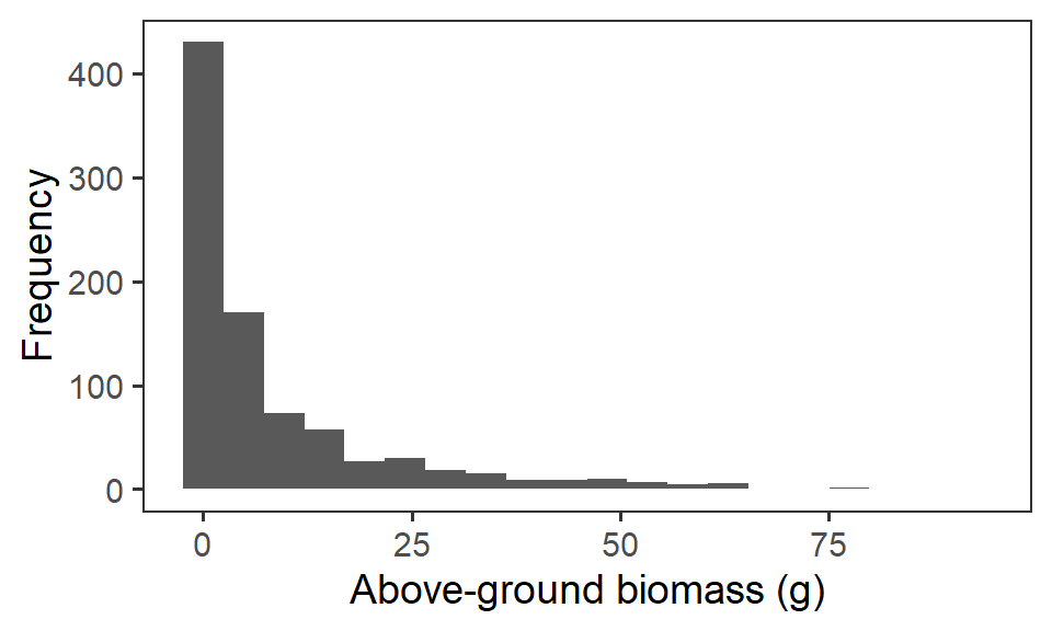
So, instead, for statistical analysis and visualisation, we take the natural logarithm \(\ln\) of the raw biomass value.
biomass <- biomass %>%
  mutate(biomass_log = log(biomass_g))

ggplot(biomass, aes(x = biomass_log)) +
  geom_histogram(bins = 20) +
  labs(x = expression(paste(ln," Above-ground biomass")), y = "Frequency") +
  theme_bw(base_size = 14) +
  theme(panel.grid = element_blank())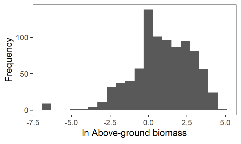
Using the ln biomass variable, we can explore patterns relating to our drought treatments, functional groups, temporal patterns and any potential block effects.
Total biomass
The first interesting question to explore is how biomass overall, which indicates primary productivity, is affected by the rainfall treatments. Here we need to sum up the biomass across functional groups. We again look at the \(\ln\) total biomass too. We present here the density plots (violins) with median (total biomass) and mean (\(\ln\) total biomass) points (large holes) as well as underlying raw data (small points).
totbiomass <- biomass %>%
  group_by(year, harvest, block, treatment) %>%
  summarise(tot_biomass = sum(biomass_g),
            log_tot_biomass = log(tot_biomass)) %>%
  ungroup()
And now we can look at how this is affected by the rainfall treatments.
tb_1 <- totbiomass %>%
  ggplot(aes(x = treatment, y = tot_biomass,
             fill = treatment)) +
  geom_violin() +
  stat_summary(fun = median, geom = "point",
               size = 6, shape = 21, fill = "white") +
  geom_jitter(width = 0.1, alpha = 0.4, size = 1) +
  scale_fill_manual(values = raindrop_colours$colour,
                    guide = F) +
  labs(x = "Rainfall treatment", y = "Total above-ground biomass (g)") +
  theme_bw(base_size = 20) +
  theme(panel.grid = element_blank())

tb_2 <- totbiomass %>%
  ggplot(aes(x = treatment, y = log_tot_biomass,
             fill = treatment)) +
  geom_violin() +
  stat_summary(fun = mean, geom = "point",
               size = 6, shape = 21, fill = "white") +
  geom_jitter(width = 0.1, alpha = 0.4, size = 1)+
  scale_fill_manual(values = raindrop_colours$colour,
                    guide = F) +
  labs(x = "Rainfall treatment",
       y = expression(paste(ln, " Total above-ground biomass"))) +
  theme_bw(base_size = 20) +
  theme(panel.grid = element_blank())

tb_1 + tb_2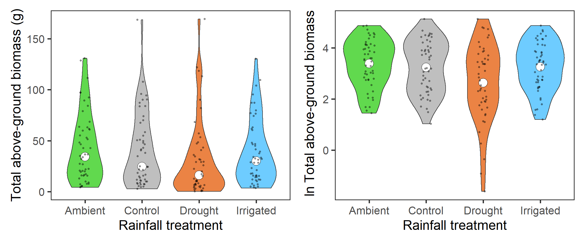
Across all functional groups, years and blocks, it looks like there is a reduction in total biomass associated with the drought treatment.
Now we’ll look at potential temporal effects i.e. whether there is a change in total biomass over time. We first have to add in temporal information to the year and harvest columns, and then we can plot out the total biomass.
# adding temporal information
totbiomass <- totbiomass %>%
  mutate(month = if_else(harvest == "End", 9, 6),
         date = as.Date(paste0(year,"-",month,"-15")),
         harvest = factor(harvest, levels = c("Mid", "End")))

# plots
totbiomass %>%
  ggplot(aes(x = date, y = log_tot_biomass, colour = treatment,
             group = treatment, shape = harvest)) +
  stat_summary(geom = "line", fun = mean, size = 0.9) +
  stat_summary(geom = "point", fun = mean, size = 3) +
  scale_colour_manual(values = raindrop_colours$colour) +
  labs(x = "Year", y = expression(paste("Mean ", ln, " total biomass")),
       colour = "Treatment", shape = "Harvest") +
  theme_bw(base_size = 14) +
  theme(panel.grid = element_blank())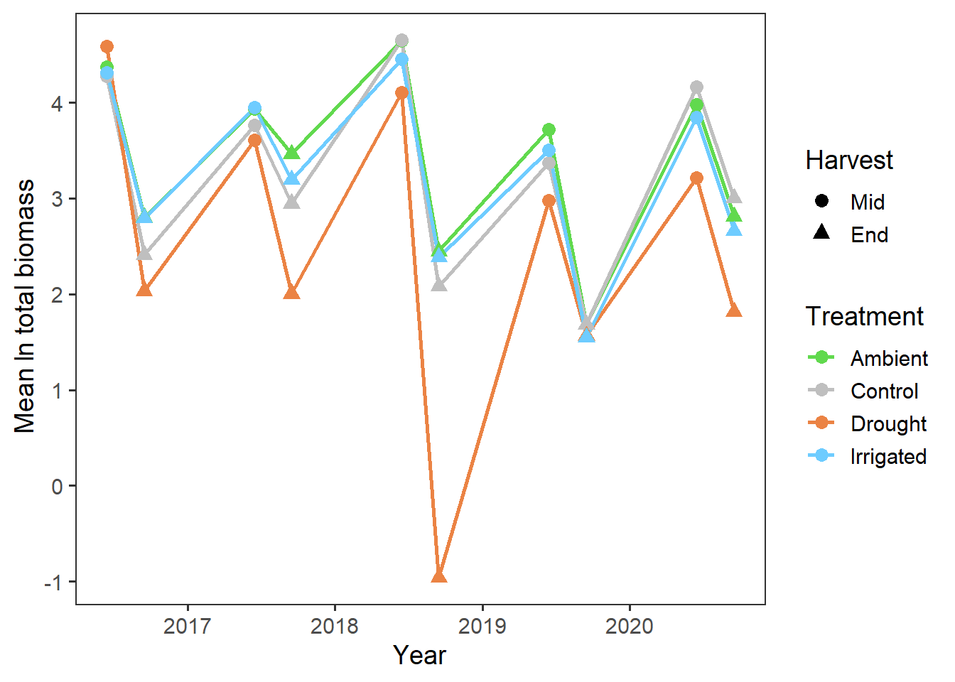
And also splitting out the harvests, as the end of the growing season has lower biomass
totbiomass %>%
  ggplot(aes(x = year, y = log_tot_biomass, colour = treatment,
             group = treatment)) +
  stat_summary(geom = "line", fun = mean, size = 0.9) +
  stat_summary(geom = "point", fun = mean, size = 3) +
  scale_colour_manual(values = raindrop_colours$colour) +
  labs(x = "Year", y = expression(paste("Mean ", ln, " total biomass")),
       colour = "Treatment") +
  facet_wrap(~harvest) +
  theme_bw(base_size = 20) +
  theme(panel.grid = element_blank(),
        strip.background = element_blank())
It looks like there may have been declines in total biomass over the years (perhaps reflecting wider climatic patterns?), but this also seems to be more prominent in the drought treatment.
Finally for total biomass, we want to look if we have any evidence for block effects at the experimental site. Here we will repeat the first treatment violin plot, but splitting by block. Here each violin is a different block (A-E from left to right) with the 50% quantile.
totbiomass %>%
  ggplot(aes(x = treatment, y = log_tot_biomass,
             fill = treatment,
             group = interaction(treatment, block))) +
  geom_violin(draw_quantiles = 0.5) +
  scale_fill_manual(values = raindrop_colours$colour,
                    guide = F) +
  labs(x = "Rainfall treatment",
       y = expression(paste(ln, " Total above-ground biomass"))) +
  theme_bw(base_size = 14) +
  theme(panel.grid = element_blank())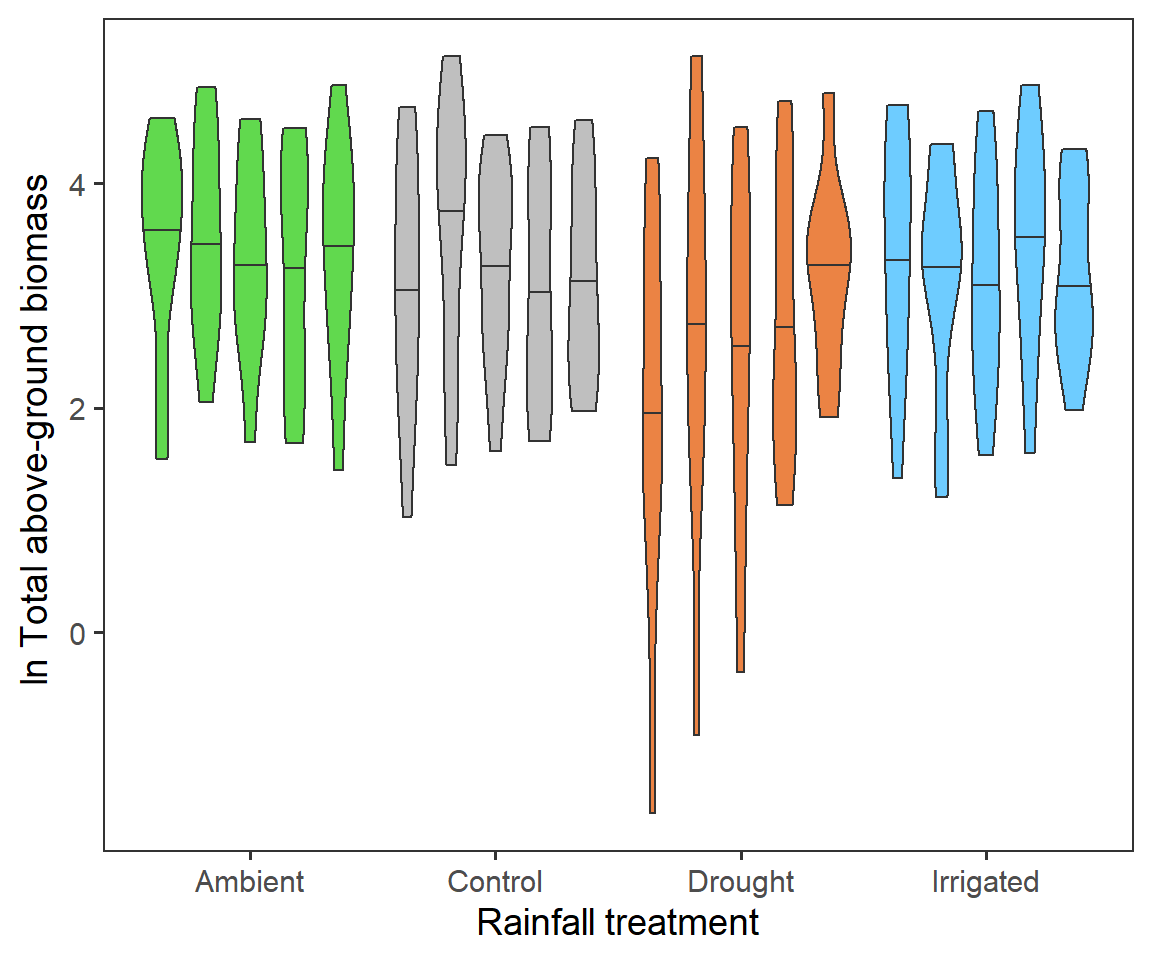
It seems that largely blocks are consistent across the RainDrop site.
Group-level biomass
Now we can go a little further and look at whether we observe any differences in biomass between different functional groups, which occur at different proportions. First, lets look at the overall differences in biomass, or relative biomass, between functional groups.
biomass %>%
  ggplot(aes(x = group, y = biomass_log,
             fill = group)) +
  geom_violin() +
  stat_summary(fun = mean, geom = "point",
               size = 5, shape = 21, fill = "white") +
  geom_jitter(width = 0.15, alpha = 0.2, size = 1) +
  scale_fill_brewer(palette = "Set2", guide = F) +
  labs(x = "Functional group",
       y = expression(paste(ln, " Above-ground biomass"))) +
  theme_bw(base_size = 14) +
  theme(panel.grid = element_blank())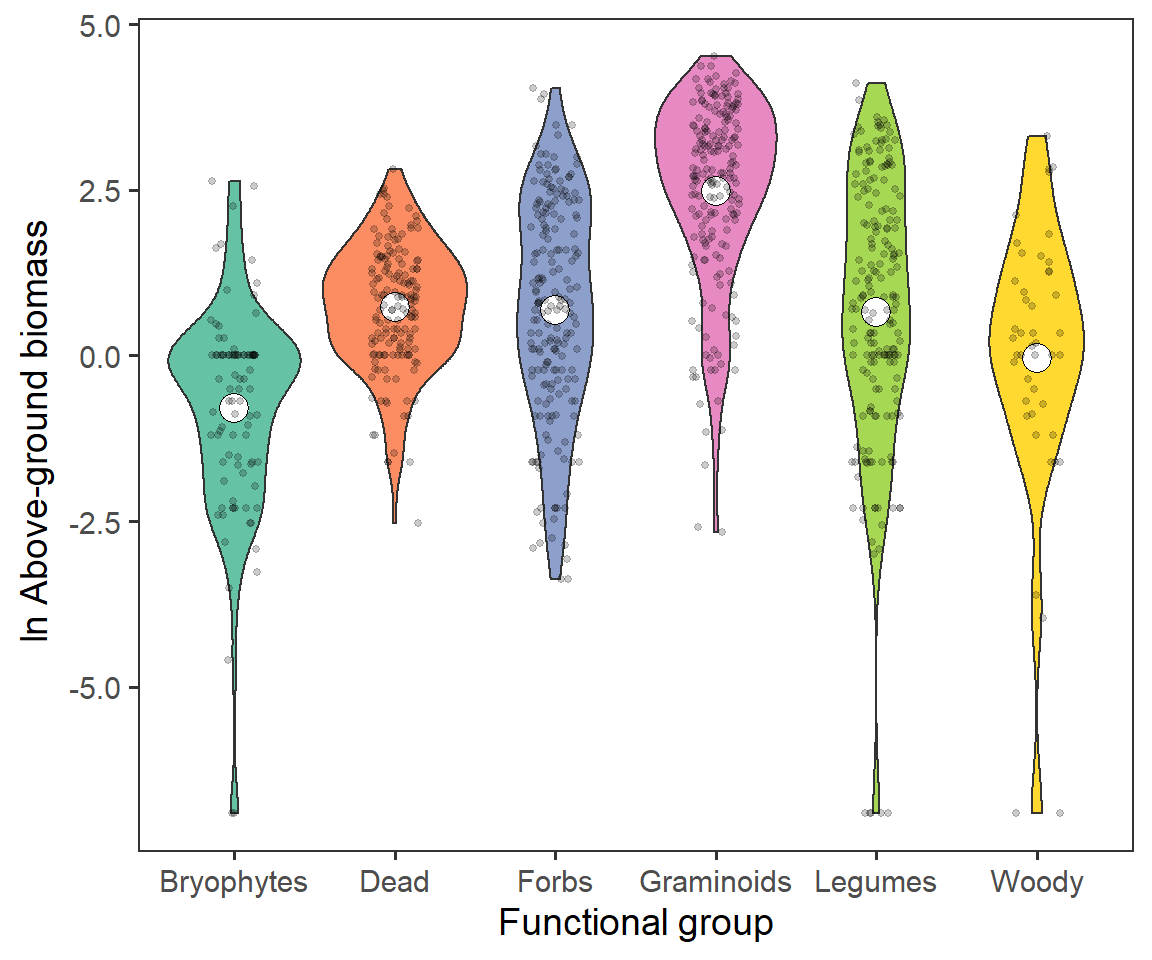
We can see that there is a large representation (as expected) of Graminoids, and lower representation of Woody species and Bryophytes.
Now lets look at the rainfall treatments by functional group.
biomass %>%
  ggplot(aes(x = treatment, y = biomass_log,
             fill = treatment)) +
  geom_violin() +
  stat_summary(fun = mean, geom = "point",
               size = 5, shape = 21, fill = "white") +
  geom_jitter(width = 0.15, alpha = 0.2, size = 1) +
  scale_fill_manual(values = raindrop_colours$colour,
                    guide = F) +
  labs(x = "Rainfall treatment",
       y = expression(paste(ln, " Above-ground biomass"))) +
  facet_wrap(~ group, ncol = 2) +
  theme_bw(base_size = 22) +
  theme(panel.grid = element_blank(),
        strip.background = element_blank())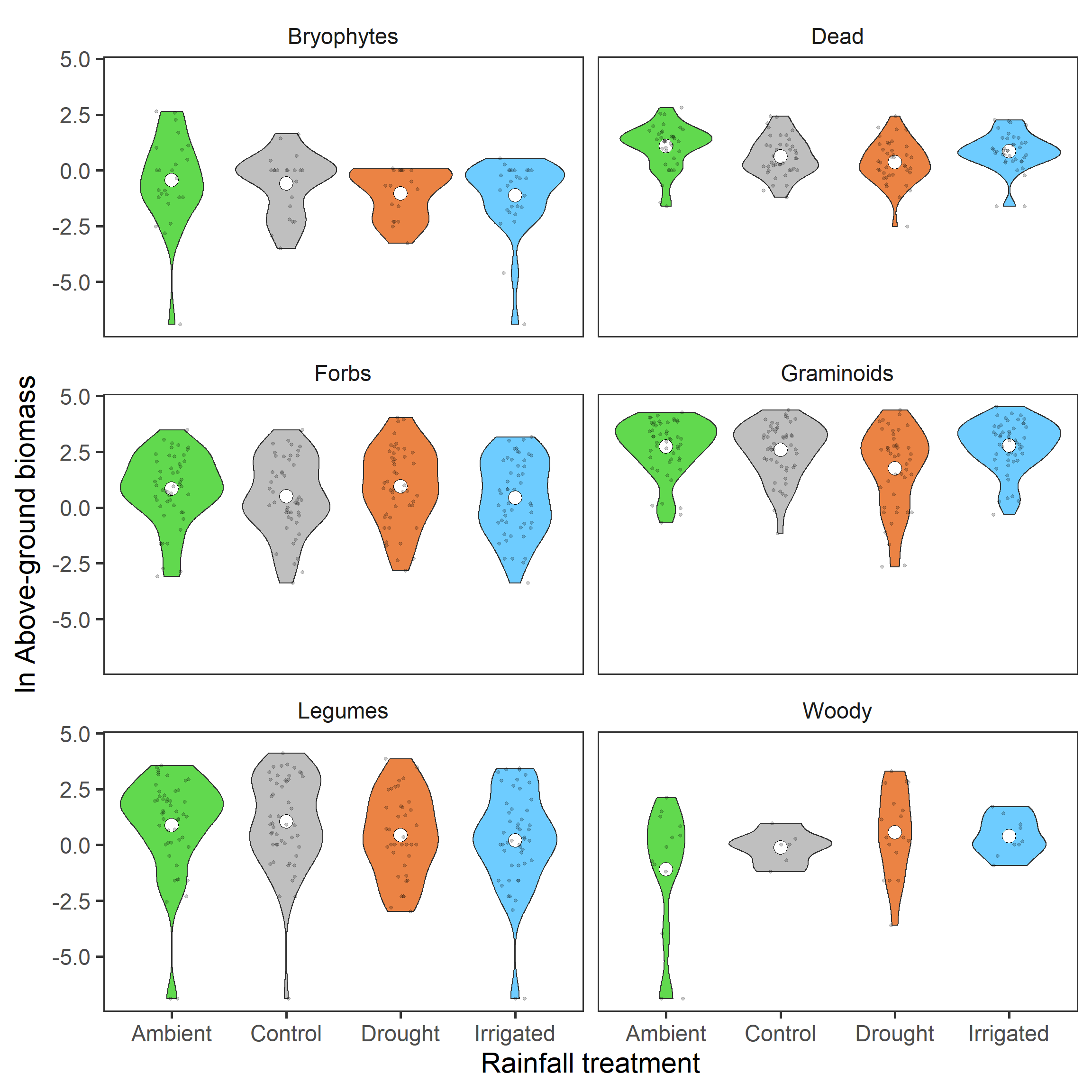
It isn’t as clear hear as total biomass. However, for the group with the most representation, the Graminoids, this reduction in the drought treatment looks to be maintained.
Finally we can look at whether there are differences in the temporal patterns between the functional groups.
# adding temporal information
biomass <- biomass %>%
  mutate(month = if_else(harvest == "End", 9, 6),
         date = as.Date(paste0(year,"-",month,"-15")),
         harvest = factor(harvest, levels = c("Mid", "End")))

# plot
biomass %>%
  ggplot(aes(x = date, y = biomass_log, colour = treatment,
             group = treatment, shape = harvest)) +
  stat_summary(geom = "line", fun = mean, size = 0.9) +
  stat_summary(geom = "point", fun = mean, size = 3) +
  scale_colour_manual(values = raindrop_colours$colour) +
  facet_wrap(~group) +
  labs(x = "Year", y = expression(paste(ln, " Above-ground biomass")),
       colour = "Treatment", shape = "Harvest") +
  theme_bw(base_size = 22) +
  theme(panel.grid = element_blank(),
        strip.background = element_blank())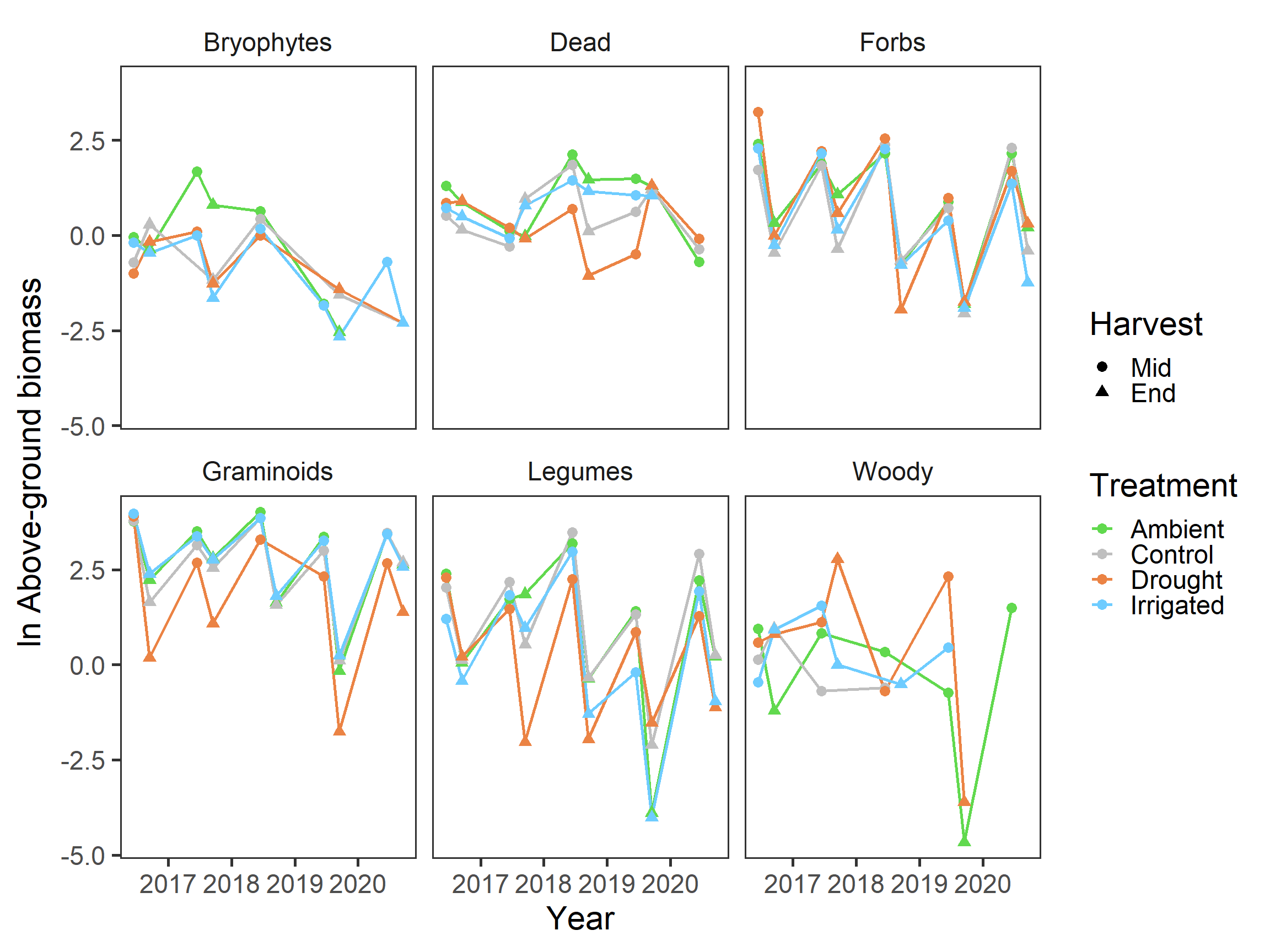
Again, specific patterns are hard to discern here, but it looks like biomass is decreasing slightly again in general.
2. Species diversity
Data summary
The species diversity data is in in the form of percentage cover of individually id’ species in a 1m x 1m quadrant in the center of each experimental plot. These percentage cover measurements were generally made at the peak of the growing season (June), but in 2016 there were recordings in both June and September.
Here a summary of the data:
glimpse(percent_cover)Rows: 2,956
Columns: 8
$ year <dbl> 2018, 2016, 2016, 2016, 2016, 2016, 2016, 2016, 2016, 20~
$ month <chr> "June", "June", "June", "June", "June", "June", "June", ~
$ block <chr> "C", "B", "B", "C", "E", "A", "E", "C", "D", "B", "D", "~
$ treatment <chr> "Control", "Ambient", "Control", "Irrigated", "Control",~
$ species_level <chr> "No", "Yes", "Yes", "Yes", "Yes", "Yes", "Yes", "Yes", "~
$ species <chr> "Acer_sp", "Agrimonia_eupatoria", "Agrimonia_eupatoria",~
$ plant_type <chr> NA, "Forb", "Forb", "Forb", "Forb", "Forb", "Forb", "For~
$ percent_cover <dbl> 1.0, 1.0, 2.0, 4.0, 4.0, 5.0, 5.0, 7.0, 8.0, 10.0, 15.0,~- $year - year of measurement (integer 2016-2020)
- $month - month of measurement (category “June” and “Sept”)
- $block - block of experiment (category A-E)
- $treatment - experimental treatment for Drought-Net (category “Ambient”, “Control”, “Drought” and “Irrigated”)
- $species_level - Was the measurement made at the level of species? (category “Yes”, “No”)
- $species - Binomial name of species recorded in the measurement (category, 138 unique records)
- $plant_type - Functional group/plant type of the species recorded (category “Forb”, “Grass”, “Woody”, “Legume”)
- $percent_cover - percentage cover of the species in a 1m x 1m quadrat
For the purpose of analysis here, we are interested in species diversity, and so we only want to include observations for which we have species-level data. Also, we want to clean any NA observations.
percent_cover <- percent_cover %>%
  drop_na(percent_cover) %>%
  filter(species_level == "Yes")
Diversity Indices
Our first key question regarding the percentage cover is how the rainfall treatments are influencing the community diversity of the plots. For this we will calculate some key biodiversity indices:
Species richness \(R = \text{number of types (i.e. species)}\)
Simpsons index \(\lambda = \sum_{i = 1}^{R} p_i^2\)
Shannon-Wiener index \(H' = - \sum_{i = 1}^{R}p_i\ln p_i\)
where \(p_i\) is the relative proportion of type (here species) \(i\).
Here we calculate these diversity indices for each plot (i.e. each year, month, block, treatment combination)
diversity <- percent_cover %>%
  # first convert percentages to a proportion
  mutate(proportion = percent_cover/100) %>%
  group_by(year, month, block, treatment) %>%
  # diversity indices for each group
  summarise(richness = n(),
            simpsons = sum(proportion^2),
            shannon = -sum(proportion * log(proportion))) %>%
  ungroup() %>%
  pivot_longer(cols = c(richness, simpsons, shannon),
               names_to = "index") %>%
  mutate(index_lab = case_when(
    index == "richness" ~ "Species richness",
    index == "simpsons" ~ "Simpson's index",
    index == "shannon" ~ "Shannon-Wiener index"
  ))
Diversity indices exploratory plots
Now we can explore how the diversity indices for each plot are related to the experimental treatments, temporal patterns, and any block effects.
First the treatment effects
diversity %>%
  ggplot(aes(x = treatment, y = value,
             fill = treatment)) +
  geom_violin() +
  stat_summary(fun = mean, geom = "point",
               size = 6, shape = 21, fill = "white") +
  geom_jitter(width = 0.1, alpha = 0.4, size = 1) +
  scale_fill_manual(values = raindrop_colours$colour,
                    guide = F) +
  labs(x = "Rainfall treatment", y = "Species diverity index") +
  facet_wrap(~index_lab, ncol = 1, scales = "free") +
  theme_bw(base_size = 20) +
  theme(panel.grid = element_blank(),
        strip.background = element_blank())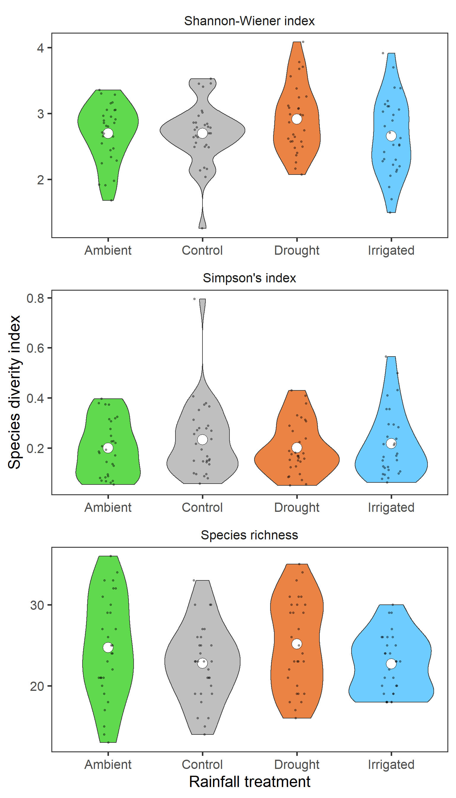
There isn’t a clear pattern here. But interestingly, it actually looks like for Shannon-Wiener, diversity is greatest in the drought treatment.
And now for potential temporal patterns
diversity %>%
  mutate(month = if_else(month == "June", 6, 9),
         date = as.Date(paste0(year,"-",month,"-15"))) %>%
  ggplot(aes(x = date, y = value, colour = treatment)) +
  stat_summary(geom = "line", fun = mean, size = 0.9) +
  stat_summary(geom = "point", fun = mean, size = 3) +
  scale_colour_manual(values = raindrop_colours$colour) +
  labs(x = "Year", y = "Mean diversity index", colour = "Treatment") +
  facet_wrap(~ index_lab, scales = "free", ncol = 1) +
  theme_bw(base_size = 20) +
  theme(panel.grid = element_blank(),
        strip.background = element_blank())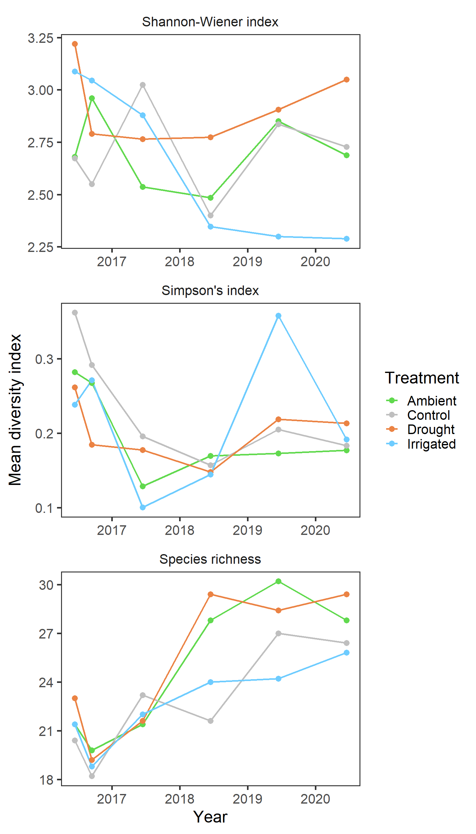
Again clear patterns are not sticking out with general indices. And finally we explore any potential block effects
diversity %>%
  ggplot(aes(x = treatment, y = value,
             fill = treatment,
             group = interaction(treatment, block))) +
  geom_violin(draw_quantiles = 0.5) +
  scale_fill_manual(values = raindrop_colours$colour,
                    guide = F) +
  labs(x = "Rainfall treatment",
       y = "Species diversity index") +
  facet_wrap(~ index_lab, scales = "free", ncol = 1) +
  theme_bw(base_size = 20) +
  theme(panel.grid = element_blank(),
        strip.background = element_blank())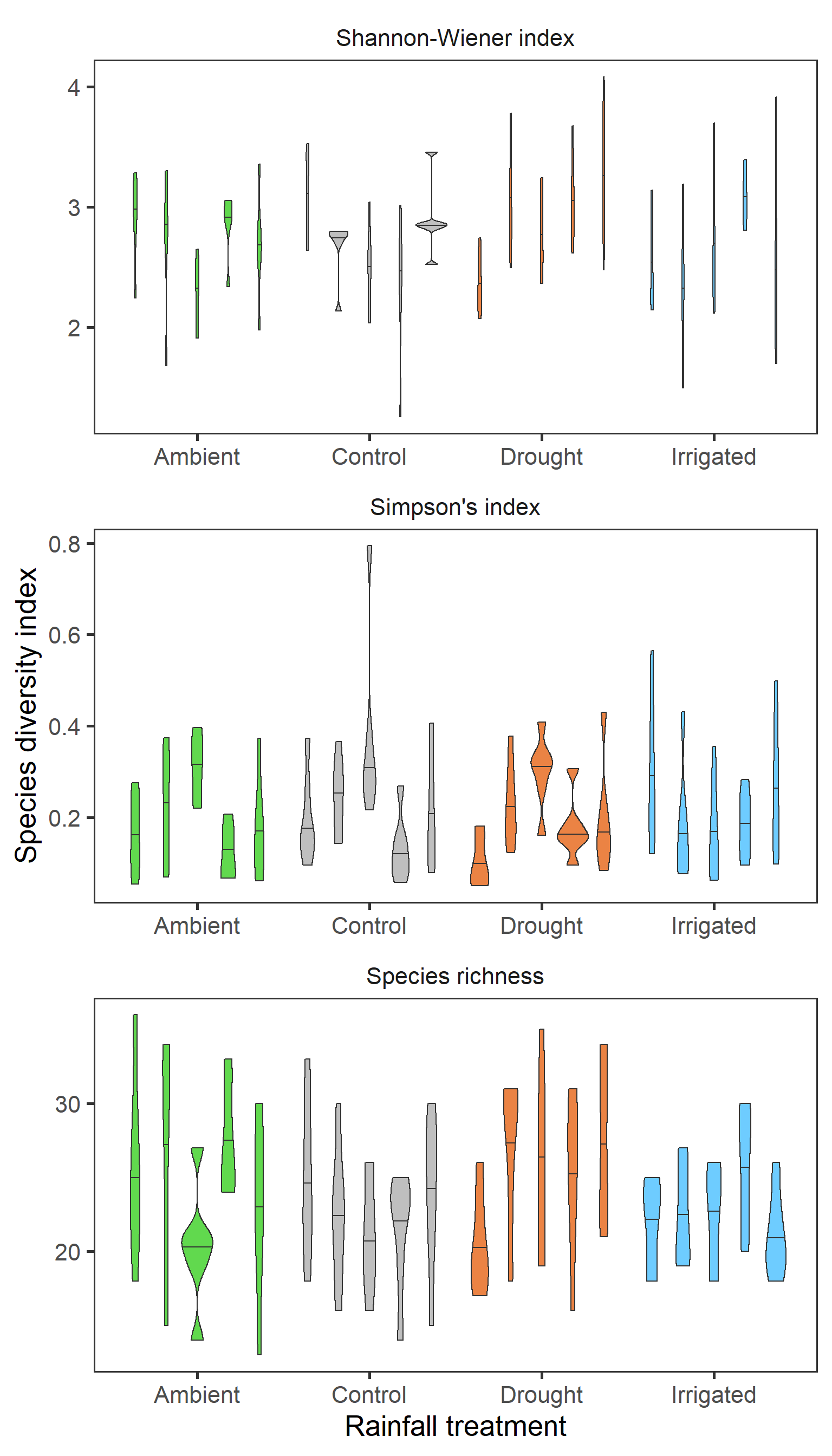
Community structure
While there may not be overall patterns in species diversity, what is interesting whether there are shifts to community structure. So, here we can perform a simple non-metric multidimensional scaling (NMDS) analysis, to look at changes to community structure with our treatments, general plant types, and also whether there are key species.
Here we perform the NMDS analysis using the vegan package, with two dimensions for 122 species in total and using the default bray distances. Firstly some cleaning though, to convert the percent cover data to a species by sample (our plots) matrix.
# data frame of the community matrix
species_community_df <- percent_cover %>%
  mutate(sample = paste(month, year, block, treatment, sep = "_")) %>%
  filter(species_level == "Yes") %>%
  dplyr::select(sample, species, percent_cover) %>%
  pivot_wider(id_cols = sample, names_from = species, values_from = percent_cover,
              values_fill = 0)

# convert to a matrix
species_community_mat <- as.matrix(species_community_df[,2:123])
rownames(species_community_mat) <- species_community_df$sample

# have a look
glimpse(species_community_mat)
num [1:120, 1:122] 1 2 4 4 5 5 7 8 10 15 ...
- attr(*, "dimnames")=List of 2
..$ : chr [1:120] "June_2016_B_Ambient" "June_2016_B_Control" "June_2016_C_Irrigated" "June_2016_E_Control" ...
..$ : chr [1:122] "Agrimonia_eupatoria" "Agrimonia_eupatorium" "Agrostis_capillaris" "Agrostis_stolonifera" ...# the NMDS
raindrop_NMDS <- metaMDS(species_community_mat, k = 2, trymax = 500)Square root transformation
Wisconsin double standardization
Run 0 stress 0.2767962
Run 1 stress 0.277602
Run 2 stress 0.2932021
Run 3 stress 0.2853559
Run 4 stress 0.2978406
Run 5 stress 0.2955674
Run 6 stress 0.2770975
... Procrustes: rmse 0.02702161 max resid 0.2110902
Run 7 stress 0.2961353
Run 8 stress 0.2805795
Run 9 stress 0.3132602
Run 10 stress 0.2992073
Run 11 stress 0.2816689
Run 12 stress 0.286314
Run 13 stress 0.2841294
Run 14 stress 0.2867314
Run 15 stress 0.3167791
Run 16 stress 0.2846884
Run 17 stress 0.3013173
Run 18 stress 0.2769089
... Procrustes: rmse 0.03336828 max resid 0.283892
Run 19 stress 0.2839498
Run 20 stress 0.2758683
... New best solution
... Procrustes: rmse 0.01609963 max resid 0.1033264
Run 21 stress 0.2825197
Run 22 stress 0.2849962
Run 23 stress 0.2825475
Run 24 stress 0.2769696
Run 25 stress 0.2826515
Run 26 stress 0.2870934
Run 27 stress 0.2861942
Run 28 stress 0.2787106
Run 29 stress 0.2806181
Run 30 stress 0.2970536
Run 31 stress 0.2853741
Run 32 stress 0.2870647
Run 33 stress 0.2827175
Run 34 stress 0.3162331
Run 35 stress 0.2939082
Run 36 stress 0.2814939
Run 37 stress 0.281456
Run 38 stress 0.2863874
Run 39 stress 0.2824177
Run 40 stress 0.2767683
Run 41 stress 0.2769162
Run 42 stress 0.2947656
Run 43 stress 0.4135299
Run 44 stress 0.2831778
Run 45 stress 0.2824217
Run 46 stress 0.3100015
Run 47 stress 0.2837495
Run 48 stress 0.2803849
Run 49 stress 0.2761917
... Procrustes: rmse 0.01950759 max resid 0.1959354
Run 50 stress 0.2844196
Run 51 stress 0.276545
Run 52 stress 0.2768445
Run 53 stress 0.280588
Run 54 stress 0.2766072
Run 55 stress 0.2850416
Run 56 stress 0.2898506
Run 57 stress 0.2939252
Run 58 stress 0.2813066
Run 59 stress 0.2776316
Run 60 stress 0.2854541
Run 61 stress 0.286179
Run 62 stress 0.2788558
Run 63 stress 0.2760823
... Procrustes: rmse 0.02841787 max resid 0.2148264
Run 64 stress 0.2951946
Run 65 stress 0.291162
Run 66 stress 0.2769294
Run 67 stress 0.2759591
... Procrustes: rmse 0.02819276 max resid 0.2160721
Run 68 stress 0.2816072
Run 69 stress 0.2817325
Run 70 stress 0.2993286
Run 71 stress 0.2823217
Run 72 stress 0.3138409
Run 73 stress 0.2756409
... New best solution
... Procrustes: rmse 0.006688926 max resid 0.05479494
Run 74 stress 0.2857355
Run 75 stress 0.2834664
Run 76 stress 0.2834251
Run 77 stress 0.2954893
Run 78 stress 0.286071
Run 79 stress 0.2884071
Run 80 stress 0.3051241
Run 81 stress 0.2816083
Run 82 stress 0.2829201
Run 83 stress 0.3141665
Run 84 stress 0.2783938
Run 85 stress 0.2818005
Run 86 stress 0.2831755
Run 87 stress 0.2763259
Run 88 stress 0.2888579
Run 89 stress 0.3062602
Run 90 stress 0.2856563
Run 91 stress 0.2895439
Run 92 stress 0.275793
... Procrustes: rmse 0.02787599 max resid 0.2133164
Run 93 stress 0.2856758
Run 94 stress 0.292898
Run 95 stress 0.2863794
Run 96 stress 0.2764144
Run 97 stress 0.2774566
Run 98 stress 0.2990053
Run 99 stress 0.286001
Run 100 stress 0.2800643
Run 101 stress 0.2995309
Run 102 stress 0.2854035
Run 103 stress 0.313981
Run 104 stress 0.2802067
Run 105 stress 0.2769166
Run 106 stress 0.2871338
Run 107 stress 0.301517
Run 108 stress 0.2813973
Run 109 stress 0.2803757
Run 110 stress 0.2825412
Run 111 stress 0.2819544
Run 112 stress 0.3106356
Run 113 stress 0.2857158
Run 114 stress 0.28054
Run 115 stress 0.2847235
Run 116 stress 0.2963966
Run 117 stress 0.2764471
Run 118 stress 0.2916034
Run 119 stress 0.2862926
Run 120 stress 0.2822926
Run 121 stress 0.2854575
Run 122 stress 0.2837994
Run 123 stress 0.2888163
Run 124 stress 0.2937464
Run 125 stress 0.2752022
... New best solution
... Procrustes: rmse 0.01839457 max resid 0.1949325
Run 126 stress 0.2782642
Run 127 stress 0.2903909
Run 128 stress 0.2849397
Run 129 stress 0.277819
Run 130 stress 0.2917427
Run 131 stress 0.2928313
Run 132 stress 0.3075153
Run 133 stress 0.2837128
Run 134 stress 0.2818714
Run 135 stress 0.3225496
Run 136 stress 0.2945228
Run 137 stress 0.3009094
Run 138 stress 0.2869416
Run 139 stress 0.2864973
Run 140 stress 0.2871134
Run 141 stress 0.2756778
... Procrustes: rmse 0.01598282 max resid 0.1684395
Run 142 stress 0.2896974
Run 143 stress 0.2817277
Run 144 stress 0.2763396
Run 145 stress 0.2856764
Run 146 stress 0.285556
Run 147 stress 0.3037158
Run 148 stress 0.2832145
Run 149 stress 0.3136607
Run 150 stress 0.2773844
Run 151 stress 0.2832705
Run 152 stress 0.2757909
Run 153 stress 0.276911
Run 154 stress 0.2761916
Run 155 stress 0.2753927
... Procrustes: rmse 0.004412328 max resid 0.0278875
Run 156 stress 0.2815538
Run 157 stress 0.2839197
Run 158 stress 0.2776063
Run 159 stress 0.2856053
Run 160 stress 0.2909764
Run 161 stress 0.2824001
Run 162 stress 0.2945936
Run 163 stress 0.2851243
Run 164 stress 0.2952075
Run 165 stress 0.2937954
Run 166 stress 0.2821778
Run 167 stress 0.289577
Run 168 stress 0.3101815
Run 169 stress 0.2899911
Run 170 stress 0.2851066
Run 171 stress 0.2920318
Run 172 stress 0.2955044
Run 173 stress 0.2873532
Run 174 stress 0.2826145
Run 175 stress 0.2831905
Run 176 stress 0.2825163
Run 177 stress 0.2819337
Run 178 stress 0.2761917
Run 179 stress 0.293661
Run 180 stress 0.2909376
Run 181 stress 0.2966224
Run 182 stress 0.2948812
Run 183 stress 0.2902538
Run 184 stress 0.2759996
Run 185 stress 0.2883574
Run 186 stress 0.2843423
Run 187 stress 0.3000871
Run 188 stress 0.2964049
Run 189 stress 0.2876698
Run 190 stress 0.2807912
Run 191 stress 0.2866172
Run 192 stress 0.2850386
Run 193 stress 0.2768287
Run 194 stress 0.2769162
Run 195 stress 0.2914567
Run 196 stress 0.2833897
Run 197 stress 0.2853156
Run 198 stress 0.2802875
Run 199 stress 0.2820744
Run 200 stress 0.2761915
Run 201 stress 0.2831963
Run 202 stress 0.2831736
Run 203 stress 0.2767927
Run 204 stress 0.2774054
Run 205 stress 0.2756942
... Procrustes: rmse 0.01598043 max resid 0.1670758
Run 206 stress 0.2777929
Run 207 stress 0.2931061
Run 208 stress 0.2844497
Run 209 stress 0.2852446
Run 210 stress 0.2783617
Run 211 stress 0.2999261
Run 212 stress 0.2956568
Run 213 stress 0.2821161
Run 214 stress 0.2754694
... Procrustes: rmse 0.006474131 max resid 0.05279246
Run 215 stress 0.2921575
Run 216 stress 0.2831807
Run 217 stress 0.2918956
Run 218 stress 0.2851382
Run 219 stress 0.2858284
Run 220 stress 0.2933459
Run 221 stress 0.2855018
Run 222 stress 0.2816954
Run 223 stress 0.2812924
Run 224 stress 0.2817054
Run 225 stress 0.2923533
Run 226 stress 0.2841288
Run 227 stress 0.2904194
Run 228 stress 0.2813527
Run 229 stress 0.2839412
Run 230 stress 0.2815432
Run 231 stress 0.2769522
Run 232 stress 0.2797161
Run 233 stress 0.2868148
Run 234 stress 0.2788169
Run 235 stress 0.2758682
Run 236 stress 0.2878844
Run 237 stress 0.2818175
Run 238 stress 0.2802102
Run 239 stress 0.2903001
Run 240 stress 0.2852655
Run 241 stress 0.2829224
Run 242 stress 0.2883752
Run 243 stress 0.4131698
Run 244 stress 0.3148125
Run 245 stress 0.2878972
Run 246 stress 0.2809798
Run 247 stress 0.280497
Run 248 stress 0.2768593
Run 249 stress 0.2912055
Run 250 stress 0.2758684
Run 251 stress 0.2999398
Run 252 stress 0.282178
Run 253 stress 0.2870254
Run 254 stress 0.275199
... New best solution
... Procrustes: rmse 0.001180725 max resid 0.01078959
Run 255 stress 0.3084651
Run 256 stress 0.2827973
Run 257 stress 0.3013574
Run 258 stress 0.2756295
... Procrustes: rmse 0.007690206 max resid 0.05152554
Run 259 stress 0.2852168
Run 260 stress 0.2819611
Run 261 stress 0.30995
Run 262 stress 0.2902704
Run 263 stress 0.2819535
Run 264 stress 0.2825163
Run 265 stress 0.2803926
Run 266 stress 0.285498
Run 267 stress 0.2874139
Run 268 stress 0.2760015
Run 269 stress 0.294528
Run 270 stress 0.2892038
Run 271 stress 0.2757909
Run 272 stress 0.2897887
Run 273 stress 0.3042521
Run 274 stress 0.2841449
Run 275 stress 0.308743
Run 276 stress 0.2853573
Run 277 stress 0.2823228
Run 278 stress 0.2824113
Run 279 stress 0.2939282
Run 280 stress 0.2811827
Run 281 stress 0.2754026
... Procrustes: rmse 0.005491697 max resid 0.03938792
Run 282 stress 0.280312
Run 283 stress 0.2853019
Run 284 stress 0.2993653
Run 285 stress 0.2848496
Run 286 stress 0.2835985
Run 287 stress 0.2759896
Run 288 stress 0.2756956
... Procrustes: rmse 0.01607401 max resid 0.1673164
Run 289 stress 0.2836377
Run 290 stress 0.2783561
Run 291 stress 0.2965925
Run 292 stress 0.2842897
Run 293 stress 0.2753913
... Procrustes: rmse 0.005077171 max resid 0.03917087
Run 294 stress 0.2769208
Run 295 stress 0.2826611
Run 296 stress 0.2836992
Run 297 stress 0.288379
Run 298 stress 0.2783109
Run 299 stress 0.2906245
Run 300 stress 0.2925783
Run 301 stress 0.2833795
Run 302 stress 0.2788488
Run 303 stress 0.2804165
Run 304 stress 0.2768885
Run 305 stress 0.2921951
Run 306 stress 0.2817128
Run 307 stress 0.2842166
Run 308 stress 0.2816443
Run 309 stress 0.2799539
Run 310 stress 0.2761916
Run 311 stress 0.2905186
Run 312 stress 0.2792492
Run 313 stress 0.2764148
Run 314 stress 0.2768102
Run 315 stress 0.2767552
Run 316 stress 0.2757909
Run 317 stress 0.2825181
Run 318 stress 0.2827509
Run 319 stress 0.2937944
Run 320 stress 0.2756779
... Procrustes: rmse 0.01601981 max resid 0.1691432
Run 321 stress 0.280515
Run 322 stress 0.2812731
Run 323 stress 0.2796134
Run 324 stress 0.2822521
Run 325 stress 0.288614
Run 326 stress 0.287689
Run 327 stress 0.2815311
Run 328 stress 0.2893268
Run 329 stress 0.307549
Run 330 stress 0.2817905
Run 331 stress 0.2925788
Run 332 stress 0.276416
Run 333 stress 0.2923969
Run 334 stress 0.277821
Run 335 stress 0.2820126
Run 336 stress 0.2899776
Run 337 stress 0.2756919
... Procrustes: rmse 0.01878761 max resid 0.1966573
Run 338 stress 0.310885
Run 339 stress 0.2819317
Run 340 stress 0.2830859
Run 341 stress 0.2771782
Run 342 stress 0.276415
Run 343 stress 0.2810702
Run 344 stress 0.2817051
Run 345 stress 0.2976131
Run 346 stress 0.3000953
Run 347 stress 0.2854301
Run 348 stress 0.2873747
Run 349 stress 0.2840335
Run 350 stress 0.2847668
Run 351 stress 0.2877928
Run 352 stress 0.2761237
Run 353 stress 0.2816047
Run 354 stress 0.2857891
Run 355 stress 0.2967727
Run 356 stress 0.2868496
Run 357 stress 0.2760473
Run 358 stress 0.321193
Run 359 stress 0.2826918
Run 360 stress 0.2876268
Run 361 stress 0.2752018
... Procrustes: rmse 0.001113995 max resid 0.01032134
Run 362 stress 0.2824346
Run 363 stress 0.281036
Run 364 stress 0.2819728
Run 365 stress 0.2825744
Run 366 stress 0.2957984
Run 367 stress 0.2989419
Run 368 stress 0.2768681
Run 369 stress 0.2871297
Run 370 stress 0.3062691
Run 371 stress 0.287284
Run 372 stress 0.4136489
Run 373 stress 0.280988
Run 374 stress 0.2934075
Run 375 stress 0.285402
Run 376 stress 0.275641
... Procrustes: rmse 0.01855291 max resid 0.1969236
Run 377 stress 0.2907737
Run 378 stress 0.3015324
Run 379 stress 0.2897734
Run 380 stress 0.2819079
Run 381 stress 0.275199
... New best solution
... Procrustes: rmse 0.0001407104 max resid 0.0008498833
... Similar to previous best
*** Solution reachedAnd now we can pull out the NMDS scores (2 dimensions), and explore their patterns in relation to the RainDrop study. First we look at the rainfall treatments in relation to community structure.
# scores and species points
rd_scores <- as.data.frame(raindrop_NMDS$points)
rd_species <- as.data.frame(raindrop_NMDS$species)

# converting to a nice data frame
rd_scores <- rd_scores %>%
  mutate(plot = rownames(.)) %>%
  mutate(month = as.character(map(strsplit(plot, "_"), 1)),
         year = as.numeric(map(strsplit(plot, "_"), 2)),
         block = as.character(map(strsplit(plot, "_"), 3)),
         treatment = as.character(map(strsplit(plot, "_"), 4)))

# and for species
species_types <- percent_cover %>%
  group_by(species) %>%
  summarise(plant_type = plant_type[1])

rd_species <- rd_species %>%
  mutate(species = rownames(.)) %>%
  left_join(x = ., y = species_types, by = "species")

# treatment plot
rd_scores %>%
  ggplot(aes(x = MDS1, y = MDS2, colour = treatment)) +
  geom_point(alpha = 0.8, size = 4) +
  stat_ellipse(level = 0.8, size = 1, show.legend = F) +
  scale_colour_manual(values = raindrop_colours$colour) +
  labs(x = "NMDS1", y = "NMDS2", colour = "Rainfall\ntreatment") +
  theme_bw(base_size = 14) +
  theme(panel.grid = element_blank())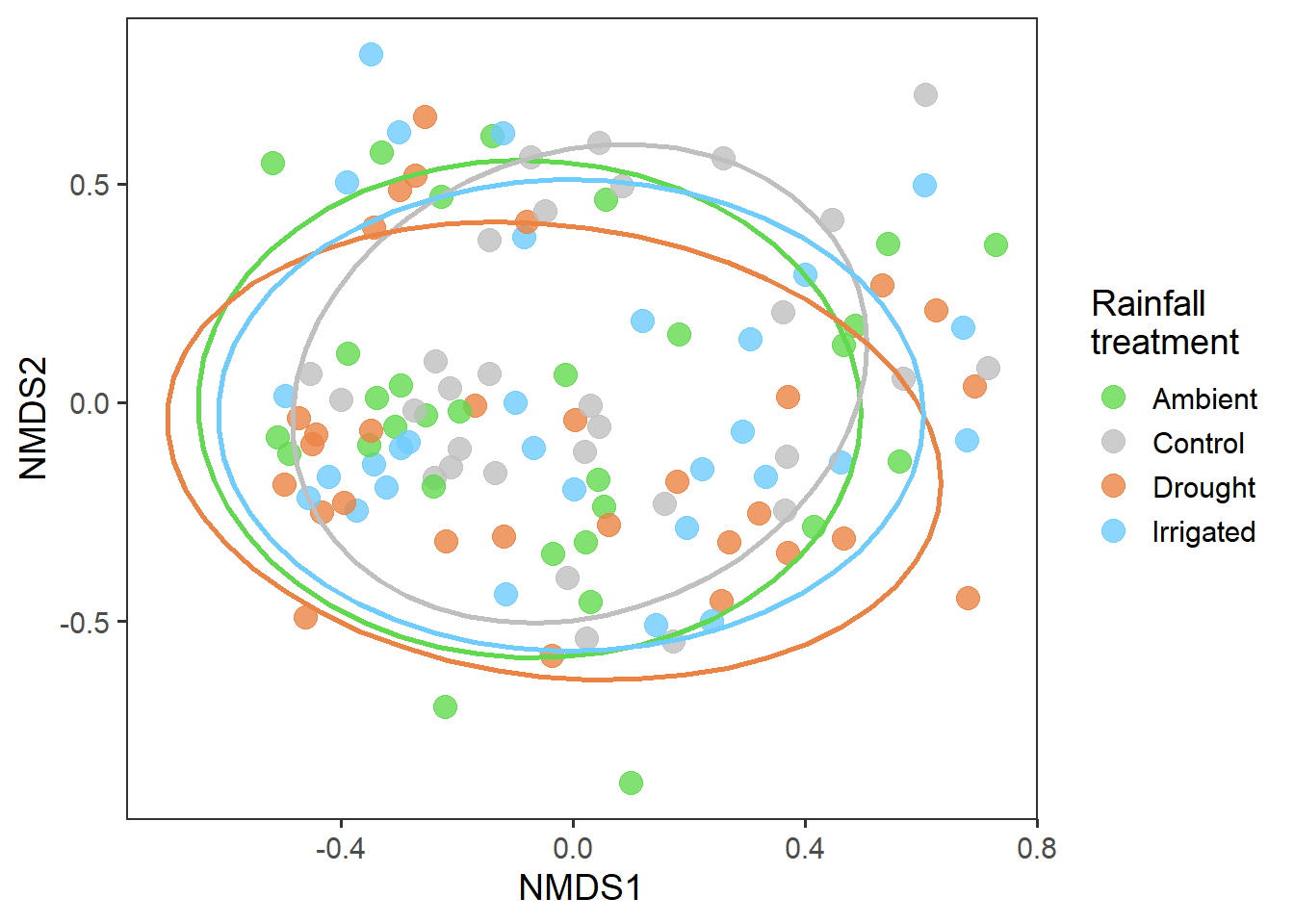
And now whether there are any interesting temporal effects
rd_scores %>%
  ggplot(aes(x = MDS1, y = MDS2, colour = as.factor(year))) +
  geom_point(alpha = 0.8, size = 4) +
  stat_ellipse(level = 0.8, size = 1, show.legend = F) +
  scale_colour_viridis_d() +
  labs(x = "NMDS1", y = "NMDS2", colour = "Year") +
  theme_bw(base_size = 14) +
  theme(panel.grid = element_blank())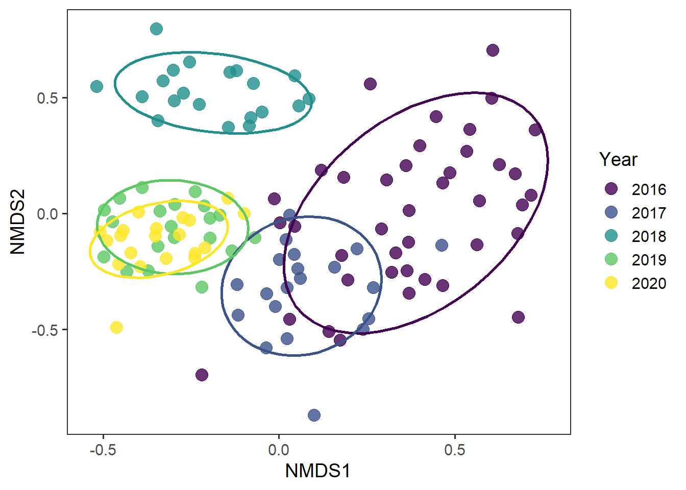
It does look like there are interesting temporal patterns in community structure here.
And we can now see whether there are important groups of species or groups of species that may be driving community structure differences. This is essentially the ‘loading’ of each species to the two NMDS axes.
# pulling the 95% quantiles to identify most extreme data
q1 <- quantile(rd_species$MDS1, c(0.025, 0.975))
q2 <- quantile(rd_species$MDS2, c(0.025, 0.975))

rd_species_extreme <- rd_species %>%
  mutate(species_lab = gsub("_", " ", species),
         extreme_species = if_else(MDS1 > q1[2] | MDS1 < q1[1] |
                                     MDS2 > q2[2] | MDS2 < q2[1],
                                   "yes", "no"))

ggplot(rd_species_extreme,
       aes(x = MDS1, y = MDS2, colour = plant_type)) +
  geom_point(alpha = 0.8, size = 4) +
  stat_ellipse(level = 0.8, size = 1, show.legend = F) +
  geom_text(data = filter(rd_species_extreme,
                          extreme_species == "yes"),
            aes(label = species_lab), nudge_y = -0.1, show.legend = F) +
  labs(x = "NMDS1", y = "NMDS2", colour = "Plant\ntype") +
  lims(x = c(-1.2,1.7)) +
  theme_bw(base_size = 14) +
  theme(panel.grid = element_blank())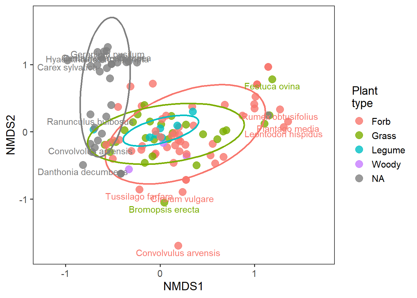
sessionInfo()R version 4.0.5 (2021-03-31)
Platform: x86_64-w64-mingw32/x64 (64-bit)
Running under: Windows 10 x64 (build 19042)
Matrix products: default
locale:
[1] LC_COLLATE=English_United Kingdom.1252
[2] LC_CTYPE=English_United Kingdom.1252
[3] LC_MONETARY=English_United Kingdom.1252
[4] LC_NUMERIC=C
[5] LC_TIME=English_United Kingdom.1252
attached base packages:
[1] stats graphics grDevices utils datasets methods base
other attached packages:
[1] vegan_2.5-7 lattice_0.20-41 permute_0.9-5 patchwork_1.1.1
[5] forcats_0.5.1 stringr_1.4.0 dplyr_1.0.5 purrr_0.3.4
[9] readr_1.4.0 tidyr_1.1.3 tibble_3.1.0 ggplot2_3.3.3
[13] tidyverse_1.3.0 workflowr_1.6.2
loaded via a namespace (and not attached):
[1] httr_1.4.2 sass_0.3.1 viridisLite_0.3.0 jsonlite_1.7.2
[5] splines_4.0.5 modelr_0.1.8 bslib_0.2.4 assertthat_0.2.1
[9] highr_0.8 cellranger_1.1.0 yaml_2.2.1 pillar_1.5.1
[13] backports_1.2.1 glue_1.4.2 digest_0.6.27 RColorBrewer_1.1-2
[17] promises_1.2.0.1 rvest_1.0.0 colorspace_2.0-0 htmltools_0.5.1.1
[21] httpuv_1.5.5 Matrix_1.3-2 pkgconfig_2.0.3 broom_0.7.5
[25] haven_2.3.1 scales_1.1.1 whisker_0.4 later_1.1.0.1
[29] git2r_0.28.0 mgcv_1.8-34 generics_0.1.0 farver_2.1.0
[33] ellipsis_0.3.1 withr_2.4.1 cli_2.3.1 magrittr_2.0.1
[37] crayon_1.4.1 readxl_1.3.1 evaluate_0.14 ps_1.6.0
[41] fs_1.5.0 fansi_0.4.2 nlme_3.1-152 MASS_7.3-53.1
[45] xml2_1.3.2 tools_4.0.5 hms_1.0.0 lifecycle_1.0.0
[49] munsell_0.5.0 reprex_2.0.0 cluster_2.1.1 compiler_4.0.5
[53] jquerylib_0.1.3 rlang_0.4.10 grid_4.0.5 rstudioapi_0.13
[57] labeling_0.4.2 rmarkdown_2.7 gtable_0.3.0 DBI_1.1.1
[61] R6_2.5.0 lubridate_1.7.10 knitr_1.31 utf8_1.2.1
[65] rprojroot_2.0.2 stringi_1.5.3 parallel_4.0.5 Rcpp_1.0.6
[69] vctrs_0.3.7 dbplyr_2.1.0 tidyselect_1.1.0 xfun_0.22