Estimating Differences in the Distribution of First-degree Relatives
Manqing Lin, Tina Lasisi
2024-12-03 14:53:59
Last updated: 2024-12-03
Checks: 6 1
Knit directory: PODFRIDGE/
This reproducible R Markdown analysis was created with workflowr (version 1.7.1). The Checks tab describes the reproducibility checks that were applied when the results were created. The Past versions tab lists the development history.
The R Markdown file has unstaged changes. To know which version of
the R Markdown file created these results, you’ll want to first commit
it to the Git repo. If you’re still working on the analysis, you can
ignore this warning. When you’re finished, you can run
wflow_publish to commit the R Markdown file and build the
HTML.
Great job! The global environment was empty. Objects defined in the global environment can affect the analysis in your R Markdown file in unknown ways. For reproduciblity it’s best to always run the code in an empty environment.
The command set.seed(20230302) was run prior to running
the code in the R Markdown file. Setting a seed ensures that any results
that rely on randomness, e.g. subsampling or permutations, are
reproducible.
Great job! Recording the operating system, R version, and package versions is critical for reproducibility.
Nice! There were no cached chunks for this analysis, so you can be confident that you successfully produced the results during this run.
Great job! Using relative paths to the files within your workflowr project makes it easier to run your code on other machines.
Great! You are using Git for version control. Tracking code development and connecting the code version to the results is critical for reproducibility.
The results in this page were generated with repository version 327d29d. See the Past versions tab to see a history of the changes made to the R Markdown and HTML files.
Note that you need to be careful to ensure that all relevant files for
the analysis have been committed to Git prior to generating the results
(you can use wflow_publish or
wflow_git_commit). workflowr only checks the R Markdown
file, but you know if there are other scripts or data files that it
depends on. Below is the status of the Git repository when the results
were generated:
Ignored files:
    Ignored:    .DS_Store
    Ignored:    .Rhistory
    Ignored:    .Rproj.user/
    Ignored:    analysis/.Rhistory
    Ignored:    data/.DS_Store

Unstaged changes:
    Modified:   analysis/relative-distribution.Rmd
Note that any generated files, e.g. HTML, png, CSS, etc., are not included in this status report because it is ok for generated content to have uncommitted changes.
These are the previous versions of the repository in which changes were
made to the R Markdown (analysis/relative-distribution.Rmd)
and HTML (docs/relative-distribution.html) files. If you’ve
configured a remote Git repository (see ?wflow_git_remote),
click on the hyperlinks in the table below to view the files as they
were in that past version.
| File | Version | Author | Date | Message |
|---|---|---|---|---|
| Rmd | e553adc | linmatch | 2024-11-21 | Update relative-distribution.Rmd |
| Rmd | e76576b | linmatch | 2024-11-21 | Update relative-distribution.Rmd |
| Rmd | 21f0f4f | linmatch | 2024-11-19 | Update relative-distribution.Rmd |
| Rmd | f583798 | linmatch | 2024-11-14 | Update relative-distribution.Rmd |
| Rmd | 900b2e4 | linmatch | 2024-11-14 | Update relative-distribution.Rmd |
| Rmd | 776920f | linmatch | 2024-11-12 | update the model fit analysis in children’s part |
| html | 776920f | linmatch | 2024-11-12 | update the model fit analysis in children’s part |
| Rmd | 06a8f96 | linmatch | 2024-11-05 | update sibling’s part |
| html | 06a8f96 | linmatch | 2024-11-05 | update sibling’s part |
| Rmd | 1741cb1 | linmatch | 2024-11-05 | fix test |
| Rmd | 4e68621 | linmatch | 2024-11-05 | fix chisq-test in cohort stability |
| html | 4e68621 | linmatch | 2024-11-05 | fix chisq-test in cohort stability |
| Rmd | 6fb5b40 | linmatch | 2024-10-29 | update sibling’s distribution plot |
| Rmd | 570abb0 | linmatch | 2024-10-22 | update sibling part |
| Rmd | 2e09e08 | linmatch | 2024-10-22 | workflow build |
| html | 2e09e08 | linmatch | 2024-10-22 | workflow build |
| Rmd | bb2c61b | linmatch | 2024-10-21 | complete fertility shift analysis |
| Rmd | 842d935 | linmatch | 2024-10-17 | update fertility shift |
| Rmd | 2ae8460 | linmatch | 2024-10-16 | fix the chisq-test |
| Rmd | 9632ae1 | linmatch | 2024-10-12 | update cohort stability |
| Rmd | 9852339 | linmatch | 2024-10-08 | update cohort stability |
| html | 9852339 | linmatch | 2024-10-08 | update cohort stability |
| Rmd | 7ec169f | linmatch | 2024-10-03 | update sibling distribution |
| Rmd | 27b986f | linmatch | 2024-10-01 | update stability cohort analysis |
| Rmd | 57a97db | linmatch | 2024-09-30 | Update relative-distribution.Rmd |
| Rmd | 52aa7f8 | linmatch | 2024-09-27 | improving code on Part1 |
| Rmd | c54a746 | linmatch | 2024-09-26 | update and fix step 2 |
| Rmd | 94d00b3 | linmatch | 2024-09-24 | fix step1 |
| Rmd | 1225480 | linmatch | 2024-09-23 | update on step1 |
| Rmd | 83174c0 | Tina Lasisi | 2024-09-22 | Instructions and layout for relative distribution |
| html | 83174c0 | Tina Lasisi | 2024-09-22 | Instructions and layout for relative distribution |
| Rmd | 78c1621 | Tina Lasisi | 2024-09-21 | Update relative-distribution.Rmd |
| Rmd | f4c2830 | Tina Lasisi | 2024-09-21 | Update relative-distribution.Rmd |
| Rmd | 2851385 | Tina Lasisi | 2024-09-21 | rename old analysis |
| html | 2851385 | Tina Lasisi | 2024-09-21 | rename old analysis |
Introduction
The relative genetic surveillance of a population is influenced by the number of genetically detectable relatives individuals have. First-degree relatives (parents, siblings, and children) are especially relevant in forensic analyses using short tandem repeat (STR) loci, where close familial searches are commonly employed. To explore potential disparities in genetic detectability between African American and European American populations, we examined U.S. Census data from four census years (1960, 1970, 1980, and 1990) focusing on the number of children born to women over the age of 40.
Data Sources
We used publicly available data from the Integrated Public Use Microdata Series (IPUMS) for the U.S. Census years 1960, 1970, 1980, and 1990. The datasets include information on:
- AGE: Age of the respondent.
- RACE: Self-identified race of the respondent.
- chborn_num: Number of children ever born to the respondent.
Data citation: Steven Ruggles, Sarah Flood, Matthew Sobek, Daniel Backman, Annie Chen, Grace Cooper, Stephanie Richards, Renae Rogers, and Megan Schouweiler. IPUMS USA: Version 14.0 [dataset]. Minneapolis, MN: IPUMS, 2023. https://doi.org/10.18128/D010.V14.0
Data Preparation
Filtering Criteria: We selected women aged 40 and above to ensure that most had completed childbearing.
Due to the terms of agreement for using this data, we cannot share the full dataset but our repo contains the subset that was used to calculate the mean number of offspring and variance.
Race Classification: We categorized individuals into two groups:
- African American: Those who identified as “Black” or “African American”.
- European American: Those who identified as “White”.
Calculating Number of Siblings: For each child of these women, the number of siblings (n_sib) is one less than the number of children born to the mother:
\[ n_{sib} = chborn_{num} - 1 \]
path <- file.path(".", "data")
savepath <- file.path(".", "output")

prop_race_year <- file.path(path, "proportions_table_by_race_year.csv")
data_filter <- file.path(path, "data_filtered_recoded.csv")

children_data = read.csv(prop_race_year)
mother_data = read.csv(data_filter)
df <- mother_data %>%
# Filter for women aged 40 and above
filter(AGE >= 40) %>%
mutate(
# Create new age ranges
AGE_RANGE = case_when(
AGE >= 70 ~ "70+",
AGE >= 60 ~ "60-69",
AGE >= 50 ~ "50-59",
AGE >= 40 ~ "40-49",
TRUE ~ as.character(AGE_RANGE) # This shouldn't occur due to the filter, but included for completeness
),
# Convert CHBORN to ordered factor
CHBORN = factor(case_when(
chborn_num == 0 ~ "No children",
chborn_num == 1 ~ "1 child",
chborn_num == 2 ~ "2 children",
chborn_num == 3 ~ "3 children",
chborn_num == 4 ~ "4 children",
chborn_num == 5 ~ "5 children",
chborn_num == 6 ~ "6 children",
chborn_num == 7 ~ "7 children",
chborn_num == 8 ~ "8 children",
chborn_num == 9 ~ "9 children",
chborn_num == 10 ~ "10 children",
chborn_num == 11 ~ "11 children",
chborn_num >= 12 ~ "12+ children"
), levels = c("No children", "1 child", "2 children", "3 children",
"4 children", "5 children", "6 children", "7 children",
"8 children", "9 children", "10 children", "11 children",
"12+ children"), ordered = TRUE),
# Ensure RACE variable is correctly formatted and filtered
RACE = factor(RACE, levels = c("White", "Black/African American"))
) %>%
# Filter for African American and European American women
filter(RACE %in% c("Black/African American", "White")) %>%
# Select and reorder columns
dplyr::select(YEAR, SEX, AGE, BIRTHYR, RACE, CHBORN, AGE_RANGE, chborn_num)
# Display the first few rows of the processed data
head(df) YEAR SEX AGE BIRTHYR RACE CHBORN AGE_RANGE chborn_num
1 1960 Female 65 1894 White No children 60-69 0
2 1960 Female 49 1911 White 2 children 40-49 2
3 1960 Female 54 1905 White No children 50-59 0
4 1960 Female 56 1903 White 1 child 50-59 1
5 1960 Female 54 1905 White 1 child 50-59 1
6 1960 Female 50 1910 White No children 50-59 0# Summary of the processed data
summary(df) YEAR SEX AGE BIRTHYR
Min. :1960 Length:1917477 Min. : 41.00 Min. :1859
1st Qu.:1970 Class :character 1st Qu.: 49.00 1st Qu.:1905
Median :1970 Mode :character Median : 58.00 Median :1916
Mean :1976 Mean : 59.24 Mean :1916
3rd Qu.:1980 3rd Qu.: 68.00 3rd Qu.:1926
Max. :1990 Max. :100.00 Max. :1949
RACE CHBORN AGE_RANGE
White :1740755 2 children :452594 Length:1917477
Black/African American: 176722 No children:343319 Class :character
3 children :335119 Mode :character
1 child :292001
4 children :204983
5 children :113593
(Other) :175868
chborn_num
Min. : 0.00
1st Qu.: 1.00
Median : 2.00
Mean : 2.57
3rd Qu.: 4.00
Max. :12.00
# Check the levels of the RACE factor
levels(df$RACE)
[1] "White" "Black/African American"# Count of observations by RACE
table(df$RACE)
                 White Black/African American
               1740755                 176722
# Count of observations by AGE_RANGE
table(df$AGE_RANGE)
 40-49  50-59  60-69    70+
529160 517620 436829 433868
Distribution of Number of Children Across Census Years
First we visualize the general trends in the frequency of the number of children for African American and European American mothers across the Census years by age group.
# Calculate proportions within each group, ensuring proper normalization
df_proportions <- df %>%
  group_by(YEAR, RACE, AGE_RANGE, chborn_num) %>%
  summarise(count = n(), .groups = "drop") %>%
  group_by(YEAR, RACE, AGE_RANGE) %>%
  mutate(proportion = count / sum(count)) %>%
  ungroup()

# Reshape data for the mirror plot
df_mirror <- df_proportions %>%
  mutate(proportion = if_else(RACE == "White", -proportion, proportion))

# Create color palette
my_colors <- colorRampPalette(c("#FFB000", "#F77A2E", "#DE3A8A", "#7253FF", "#5E8BFF"))(13)

# Create the plot
child_plot <- ggplot(df_mirror, aes(x = chborn_num, y = proportion, fill = as.factor(chborn_num))) +
  geom_col(aes(alpha = RACE)) +
  geom_hline(yintercept = 0, color = "black", size = 0.5) +
  facet_grid(AGE_RANGE ~ YEAR, scales = "free_y") +
  coord_flip() +
  scale_y_continuous(
    labels = function(x) abs(x),
    limits = function(x) c(-max(abs(x)), max(abs(x)))
  ) +
  scale_x_continuous(breaks = 0:12, labels = c(0:11, "12+")) +
  scale_fill_manual(values = my_colors) +
  scale_alpha_manual(values = c("White" = 0.7, "Black/African American" = 1), guide = "none") +
  labs(
    title = "Distribution of Number of Children by Census Year, Race, and Age Range",
    x = "Number of Children",
    y = "Proportion",
    fill = "Number of Children",
    caption = "White population shown on left (negative values), Black/African American on right (positive values)\nProportions normalized within each age range, race, and census year\nFootnote: The category '12+' includes families with 12 or more children."
  ) +
  theme_minimal() +
  theme(
    plot.title = element_text(size = 14, hjust = 0.5),
    axis.text.y = element_text(size = 8),
    strip.text = element_text(size = 10),
    legend.position = "none",
    panel.grid.major.y = element_blank(),
    panel.grid.minor.y = element_blank()
  )

print(child_plot)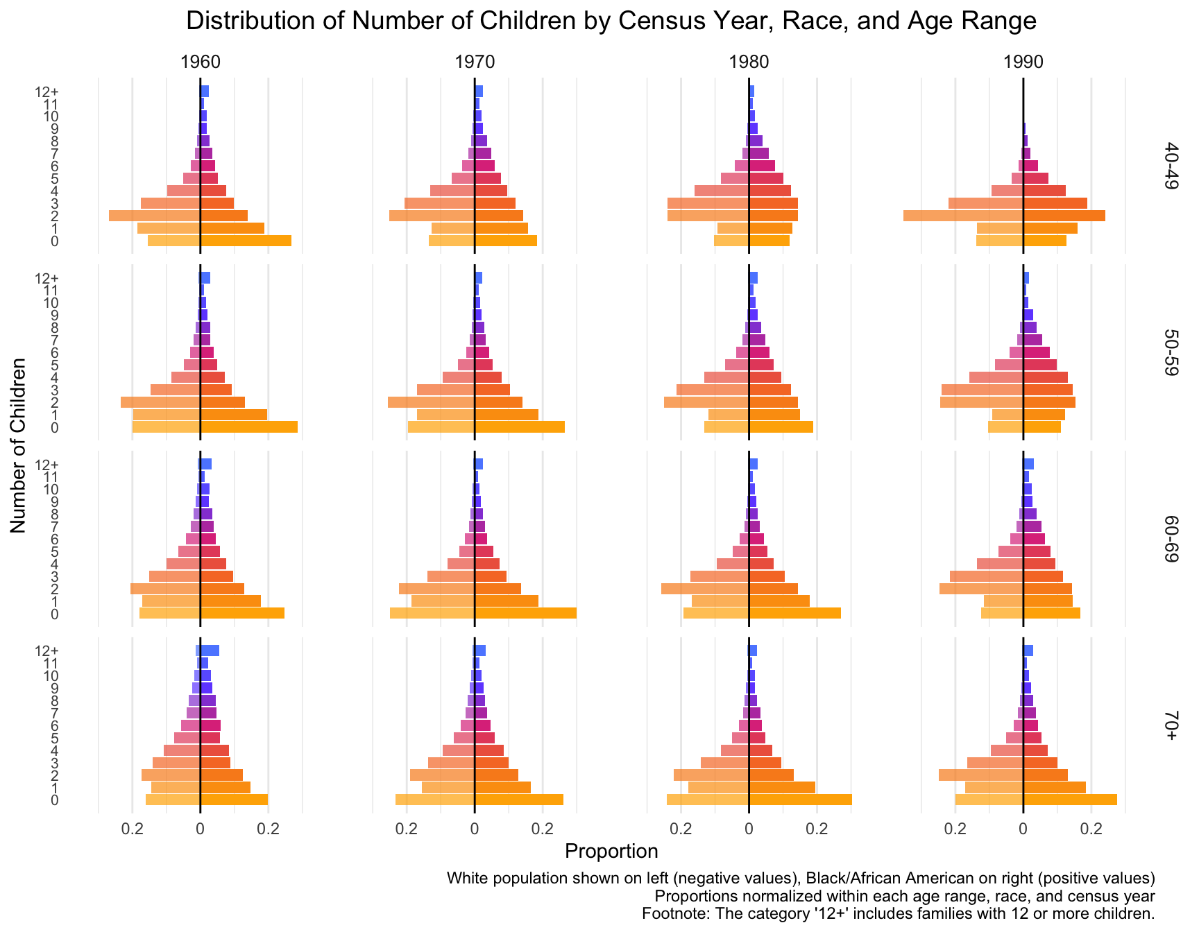
# Print summary to check age ranges and normalization
print(df_proportions %>%
  group_by(YEAR, RACE, AGE_RANGE) %>%
  summarise(total_proportion = sum(proportion), .groups = "drop") %>%
  arrange(YEAR, RACE, AGE_RANGE))
# A tibble: 32 × 4
YEAR RACE AGE_RANGE total_proportion
<int> <fct> <chr> <dbl>
1 1960 White 40-49 1
2 1960 White 50-59 1
3 1960 White 60-69 1
4 1960 White 70+ 1
5 1960 Black/African American 40-49 1
6 1960 Black/African American 50-59 1
7 1960 Black/African American 60-69 1
8 1960 Black/African American 70+ 1
9 1970 White 40-49 1
10 1970 White 50-59 1
# ℹ 22 more rowsWith this visualization of the distribution of the data, we can see that there are differences between White and Black Americans.
We will now test for differences in 1) the mean and variance, and 2) zero-inflation.
[instructions for Manqing] Model Fit Across Census Years
Question 1) What is the best model for the distribution of the data in each of these subsets of data (by race, by census year, by age range combined)?
Step 1: Fit Models Across All Subsets
For each combination of race, census year, and age range, fit your candidate models:
- Poisson Model
- Negative Binomial (NB) Model
- Zero-Inflated Poisson (ZIP) Model
- Zero-Inflated Negative Binomial (ZINB) Model
This should be done for each subset of the data (race × census year × age range).
Understanding the Data:
- Data Type: Count data representing the number of children per woman.
- Characteristics:
- Potential overdispersion (variance greater than the mean).
- Possible zero-inflation (excess zeros) in some subsets.
- Different distributions across races, census years, and age ranges.
Candidate Models for Count Data:
- Poisson Distribution:
- Assumes mean equals variance.
- Not suitable if overdispersion is present.
- Negative Binomial Distribution:
- Handles overdispersion by introducing a dispersion parameter.
- Suitable when variance exceeds the mean.
- Zero-Inflated Models:
- Zero-Inflated Poisson (ZIP):
- Combines a Poisson distribution with a point mass at zero.
- Suitable if there’s an excess of zeros.
- Zero-Inflated Negative Binomial (ZINB):
- Combines a negative binomial distribution with a point mass at zero.
- Handles both overdispersion and excess zeros.
- Zero-Inflated Poisson (ZIP):
- Hurdle Models: (optional)
- Similar to zero-inflated models but model zeros and positive counts separately.
Recommended Approach:
1: Exploratory Data Analysis (EDA)
- Compute Mean and Variance:
- For each subset (race, census year, age range), calculate the mean and variance of the number of children.
- Check for overdispersion: If variance > mean, overdispersion is present.
- Check for Zero-Inflation:
- Calculate the proportion of zeros in each subset.
- If the proportion of zeros is significantly higher than expected under a standard Poisson or negative binomial model, consider zero-inflated models.
2: Model Selection
Scenario 1: Overdispersion Without Excess Zeros
- Model: Negative Binomial Distribution
- Justification: Handles overdispersion effectively.
Scenario 2: Overdispersion With Excess Zeros
- Model: Zero-Inflated Negative Binomial (ZINB) Distribution
- Justification: Accounts for both overdispersion and excess zeros.
Scenario 3: No Overdispersion, No Excess Zeros
- Model: Poisson Distribution
- Justification: Appropriate if mean equals variance and no excess zeros.
3: Fit Models to Each Subset
- For Each Subset:
- Fit a Poisson model.
- Fit a Negative Binomial model.
- If necessary, fit a Zero-Inflated Poisson (ZIP) and Zero-Inflated Negative Binomial (ZINB) model.
- Compare Models:
- Use goodness-of-fit measures such as Akaike Information Criterion (AIC) or Bayesian Information Criterion (BIC).
- Lower AIC/BIC indicates a better-fitting model.
- Perform likelihood ratio tests where appropriate.
Step 2: Model Comparison Using AIC or BIC
Once the models are fitted, compare them using goodness-of-fit criteria like AIC or BIC for each subset. The model with the lowest AIC/BIC is the best fit for that subset.
- Assess Model Fit:
- Check residuals for patterns.
- Use diagnostic plots.
- Check Dispersion Parameter:
- For negative binomial models, examine the estimated dispersion parameter.
- Vuong Test:
- Compare zero-inflated models to standard models to assess if zero-inflation significantly improves the fit.
## Approach 1:
combinations <- df %>%
  group_by(YEAR, RACE, AGE_RANGE) %>%
  group_split()

# Initialize the data frame for storing results
EDA_df <- data.frame(
  Race = character(),
  Census_Year = numeric(),
  Age_Range = character(),
  Overdispersion = logical(),
  Zero_Inflation = logical(),
  stringsAsFactors = FALSE
)

# Initialize vectors for overdispersion and zero-inflation
overdispersion <- logical(length(combinations))
zero_inflation <- logical(length(combinations))

for (i in seq_along(combinations)) {
  subset_data <- combinations[[i]]
  mean_chborn <- mean(subset_data$chborn_num)
  var_chborn <- var(subset_data$chborn_num)

  # Check for overdispersion (variance > mean)
  overdispersion[i] <- var_chborn > mean_chborn

  # Check for zero-inflation
  prop_zero <- sum(subset_data$chborn_num == 0) / nrow(subset_data)

  # Compare prop_zero to expected under Poisson
  exp_poisson <- exp(-mean_chborn)

  # Compare prop_zero to expected under Negative Binomial
  standard_nb <- glm.nb(chborn_num ~ 1, data = subset_data)
  theta_nb <- standard_nb$theta
  exp_zero_nb <- (theta_nb / (theta_nb + mean_chborn))^theta_nb

  zero_inflation[i] <- prop_zero > exp_poisson | prop_zero > exp_zero_nb

  # Store the results in the EDA_df
  EDA_df <- rbind(
    EDA_df,
    data.frame(
      Race = unique(subset_data$RACE),
      Census_Year = unique(subset_data$YEAR),
      Age_Range = unique(subset_data$AGE_RANGE),
      Overdispersion = overdispersion[i],
      Zero_Inflation = zero_inflation[i],
      stringsAsFactors = FALSE
    )
  )
}
EDA_df$model <- NA # Create an empty column for the model
for(i in 1:nrow(EDA_df)) {
if(EDA_df$Overdispersion[i] & EDA_df$Zero_Inflation[i]) {
EDA_df$model[i] <- "Zero-Inflated Negative Binomial"
} else if(EDA_df$Overdispersion[i] & !EDA_df$Zero_Inflation[i]) {
EDA_df$model[i] <- "Negative Binomial"
} else if(!EDA_df$Overdispersion[i] & !EDA_df$Zero_Inflation[i]) {
EDA_df$model[i] <- "Poisson"
} else if(!EDA_df$Overdispersion[i] & EDA_df$Zero_Inflation[i]){
EDA_df$model[i] <- "Zero-Inflated Poisson"
}
}
# View the final EDA_df
print(EDA_df) Race Census_Year Age_Range Overdispersion Zero_Inflation
1 White 1960 40-49 TRUE TRUE
2 White 1960 50-59 TRUE TRUE
3 White 1960 60-69 TRUE TRUE
4 White 1960 70+ TRUE TRUE
5 Black/African American 1960 40-49 TRUE TRUE
6 Black/African American 1960 50-59 TRUE TRUE
7 Black/African American 1960 60-69 TRUE TRUE
8 Black/African American 1960 70+ TRUE TRUE
9 White 1970 40-49 TRUE TRUE
10 White 1970 50-59 TRUE TRUE
11 White 1970 60-69 TRUE TRUE
12 White 1970 70+ TRUE TRUE
13 Black/African American 1970 40-49 TRUE TRUE
14 Black/African American 1970 50-59 TRUE TRUE
15 Black/African American 1970 60-69 TRUE TRUE
16 Black/African American 1970 70+ TRUE TRUE
17 White 1980 40-49 TRUE TRUE
18 White 1980 50-59 TRUE TRUE
19 White 1980 60-69 TRUE TRUE
20 White 1980 70+ TRUE TRUE
21 Black/African American 1980 40-49 TRUE TRUE
22 Black/African American 1980 50-59 TRUE TRUE
23 Black/African American 1980 60-69 TRUE TRUE
24 Black/African American 1980 70+ TRUE TRUE
25 White 1990 40-49 FALSE TRUE
26 White 1990 50-59 TRUE TRUE
27 White 1990 60-69 TRUE TRUE
28 White 1990 70+ TRUE TRUE
29 Black/African American 1990 40-49 TRUE TRUE
30 Black/African American 1990 50-59 TRUE TRUE
31 Black/African American 1990 60-69 TRUE TRUE
32 Black/African American 1990 70+ TRUE TRUE
model
1 Zero-Inflated Negative Binomial
2 Zero-Inflated Negative Binomial
3 Zero-Inflated Negative Binomial
4 Zero-Inflated Negative Binomial
5 Zero-Inflated Negative Binomial
6 Zero-Inflated Negative Binomial
7 Zero-Inflated Negative Binomial
8 Zero-Inflated Negative Binomial
9 Zero-Inflated Negative Binomial
10 Zero-Inflated Negative Binomial
11 Zero-Inflated Negative Binomial
12 Zero-Inflated Negative Binomial
13 Zero-Inflated Negative Binomial
14 Zero-Inflated Negative Binomial
15 Zero-Inflated Negative Binomial
16 Zero-Inflated Negative Binomial
17 Zero-Inflated Negative Binomial
18 Zero-Inflated Negative Binomial
19 Zero-Inflated Negative Binomial
20 Zero-Inflated Negative Binomial
21 Zero-Inflated Negative Binomial
22 Zero-Inflated Negative Binomial
23 Zero-Inflated Negative Binomial
24 Zero-Inflated Negative Binomial
25 Zero-Inflated Poisson
26 Zero-Inflated Negative Binomial
27 Zero-Inflated Negative Binomial
28 Zero-Inflated Negative Binomial
29 Zero-Inflated Negative Binomial
30 Zero-Inflated Negative Binomial
31 Zero-Inflated Negative Binomial
32 Zero-Inflated Negative Binomial## Approach 2
# Initialize the data frame to store results
best_models <- data.frame(
Race = character(),
Census_Year = numeric(),
Age_Range = character(),
AIC_poisson = numeric(),
AIC_nb = numeric(),
AIC_zip = numeric(),
AIC_zinb = numeric(),
stringsAsFactors = FALSE
)
# Loop through each subset of data
for (i in seq_along(combinations)) {
subset_data <- combinations[[i]]
# Fit Poisson model
poisson_model <- glm(chborn_num ~ 1, family = poisson, data = subset_data)
# Fit Negative Binomial model
nb_model <- glm.nb(chborn_num ~ 1, data = subset_data)
# Fit Zero-Inflated Poisson model
zip_model <- zeroinfl(chborn_num ~ 1 | 1, data = subset_data, dist = "poisson")
# Fit Zero-Inflated Negative Binomial model
zinb_model <- zeroinfl(chborn_num ~ 1 | 1, data = subset_data, dist = "negbin")
# Append the result to the best_models data frame
best_models <- rbind(
best_models,
data.frame(
Race = unique(subset_data$RACE),
Census_Year = unique(subset_data$YEAR),
Age_Range = unique(subset_data$AGE_RANGE),
AIC_poisson = AIC(poisson_model),
AIC_nb = AIC(nb_model),
AIC_zip = AIC(zip_model),
AIC_zinb = AIC(zinb_model),
stringsAsFactors = FALSE
)
)
}# Add a Best_Model column to store the best model based on minimum AIC
best_models$Best_Model <- apply(best_models, 1, function(row) {
# Get AIC values for Poisson, NB, ZIP, and ZINB models
aic_values <- c(Poisson = as.numeric(row['AIC_poisson']),
Negative_Binomial = as.numeric(row['AIC_nb']),
Zero_Inflated_Poisson = as.numeric(row['AIC_zip']),
Zero_Inflated_NB= as.numeric(row['AIC_zinb']))
# Find the name of the model with the minimum AIC value
best_model <- names(which.min(aic_values))
return(best_model)
})
best_models <- best_models %>% dplyr::select(Race, Census_Year, Age_Range, Best_Model)
# View the updated table with the Best_Model column
print(best_models) Race Census_Year Age_Range Best_Model
1 White 1960 40-49 Zero_Inflated_NB
2 White 1960 50-59 Zero_Inflated_NB
3 White 1960 60-69 Zero_Inflated_NB
4 White 1960 70+ Zero_Inflated_NB
5 Black/African American 1960 40-49 Zero_Inflated_NB
6 Black/African American 1960 50-59 Zero_Inflated_NB
7 Black/African American 1960 60-69 Zero_Inflated_NB
8 Black/African American 1960 70+ Zero_Inflated_NB
9 White 1970 40-49 Zero_Inflated_NB
10 White 1970 50-59 Zero_Inflated_NB
11 White 1970 60-69 Zero_Inflated_NB
12 White 1970 70+ Zero_Inflated_NB
13 Black/African American 1970 40-49 Zero_Inflated_NB
14 Black/African American 1970 50-59 Zero_Inflated_NB
15 Black/African American 1970 60-69 Zero_Inflated_NB
16 Black/African American 1970 70+ Zero_Inflated_NB
17 White 1980 40-49 Zero_Inflated_Poisson
18 White 1980 50-59 Zero_Inflated_NB
19 White 1980 60-69 Zero_Inflated_NB
20 White 1980 70+ Zero_Inflated_NB
21 Black/African American 1980 40-49 Zero_Inflated_NB
22 Black/African American 1980 50-59 Zero_Inflated_NB
23 Black/African American 1980 60-69 Zero_Inflated_NB
24 Black/African American 1980 70+ Zero_Inflated_NB
25 White 1990 40-49 Zero_Inflated_Poisson
26 White 1990 50-59 Zero_Inflated_Poisson
27 White 1990 60-69 Zero_Inflated_NB
28 White 1990 70+ Zero_Inflated_NB
29 Black/African American 1990 40-49 Zero_Inflated_NB
30 Black/African American 1990 50-59 Zero_Inflated_NB
31 Black/African American 1990 60-69 Zero_Inflated_NB
32 Black/African American 1990 70+ Zero_Inflated_NBStep 3: Record the Best Model for Each Subset
Create a table or data frame where you store the best model for each combination of race, census year, and age range based on AIC/BIC. For example:
| Race | Census Year | Age Range | Best Model |
|---|---|---|---|
| Black/African Am. | 1990 | 40-49 | Negative Binomial |
| White | 1990 | 40-49 | Zero-Inflated NB |
| White | 1980 | 50-59 | Poisson |
| … | … | … | … |
(but obviously do this as a dataframe so we can analyze it)
Step 4: Analyze the Effect of Race, Census Year, and Age Range
Once you’ve gathered the best model for each subset, you can analyze which factor (race, census year, or age range) is most influential in determining the best-fitting model.
Options for statistical analysis:
- Chi-Square Test of Independence: You can use a chi-square test to determine whether there is a significant association between race and the best-fitting model, or census year/age group and the best-fitting model. This test will help you see if certain races or age ranges are more likely to have a particular model as the best fit.
#example
# Need large sample size, warning message "Chi-squared approximation may be incorrect," usually occurs when some of the expected counts in the contingency table are too small (typically less than 5)
## Create a contingency table
#table_model_race <- table(best_models$Race, best_models$Best_Model)

# Perform chi-square test
#chisq.test(table_model_race)
Logistic Regression: You could fit a logistic regression model where the response variable is the best-fitting model (binary or multinomial) and the predictor variables are race, census year, and age range. This will allow you to quantify the effect of each variable on the model choice.
Example in R (assuming binary outcome: Poisson vs. NB):
# Recode Best_Model to a binary variable (e.g., "Zero_Inflated_NB" vs. "Other")
best_models$Best_Model_Binary <- ifelse(best_models$Best_Model == "Zero_Inflated_NB", 1, 0)

# Fit binary logistic regression
model_logistic <- glm(Best_Model_Binary ~ Race + Census_Year + Age_Range, family = binomial(), data = best_models)

# Summary of the logistic regression model
summary(model_logistic)
Call:
glm(formula = Best_Model_Binary ~ Race + Census_Year + Age_Range,
    family = binomial(), data = best_models)

Coefficients:
                             Estimate Std. Error z value Pr(>|z|)
(Intercept)                 8.741e+03  7.710e+06   0.001    0.999
RaceBlack/African American  8.903e+01  8.227e+04   0.001    0.999
Census_Year                -4.426e+00  3.902e+03  -0.001    0.999
Age_Range50-59              4.390e+01  5.002e+04   0.001    0.999
Age_Range60-69              8.990e+01  1.045e+05   0.001    0.999
Age_Range70+                8.990e+01  1.045e+05   0.001    0.999

(Dispersion parameter for binomial family taken to be 1)

    Null deviance: 1.9912e+01  on 31  degrees of freedom
Residual deviance: 2.4509e-09  on 26  degrees of freedom
AIC: 12

Number of Fisher Scoring iterations: 25RESULT:The p-value for each variable is larger than 0.05, indicating non-significant effects on best_model fitting.
Multinomial Logistic Regression (if more than two models): If you have multiple possible best-fitting models (Poisson, NB, ZIP, ZINB), you can use multinomial logistic regression to assess the impact of race, census year, and age range on model selection.
Example in R using the
nnetpackage:
## Not appropriate since only 2 levels in best_model
# Fit multinomial logistic regression
#model_multinom <- multinom(Best_Model ~ Race + Census_Year + Age_Range, data = best_model_data)

# Summary of results
#summary(model_multinom)
Step 5: Summarize the Results
- Significance of Each Variable: From the regression analysis (or chi-square tests), you can determine which variable (race, census year, or age range) has the most significant impact on the model choice.
- Effect Sizes: Logistic regression will provide coefficients that describe how much each variable influences the probability of choosing a particular model.
- Best Model by Race: You can summarize which model tends to fit best for each race across years and age groups. For example, you might find that the Negative Binomial model consistently fits the best for a specific race or age group, indicating more overdispersion in that subset.
Visualize the Results
Finally, visualize the distribution of the best-fitting models across races, census years, and age groups.
- Bar Plots: Show the proportion of each model for different races or age groups.
- Heatmap: Use a heatmap to visualize how the best model varies across race, census year, and age range.
Example of a simple bar plot in R:
model_proportions <- best_models %>%
  group_by(Race, Age_Range, Best_Model) %>%
  summarise(Count = n(), .groups = "drop") %>%
  group_by(Race, Age_Range) %>%
  mutate(Proportion = Count / sum(Count))

                                                                    ggplot(model_proportions, aes(x = Age_Range, y = Proportion, fill = Best_Model)) +
  geom_bar(stat = "identity", position = "fill") +
  facet_wrap(~ Race) +
  labs(
    title = "Proportion of Models by Race and Age Group",
    x = "Age Range",
    y = "Proportion",
    fill = "Model"
  ) +
  theme_minimal()
ggplot(best_models, aes(x = Census_Year, y = Age_Range, fill = Best_Model)) +
geom_tile(color = "white", lwd = 0.5, linetype = 1) +
facet_wrap(~Race, nrow = 2) +
scale_fill_manual(values = c("Zero_Inflated_Poisson" = "#0072B2", "Zero_Inflated_NB" = "#F0E442")) +
labs(
title = "Best Model by Race, Census Year, and Age Range",
x = "Census Year",
y = "Age Range",
fill = "Best Model"
) +
theme_minimal() +
theme(
plot.title = element_text(size = 14, face = "bold"),
legend.position = "bottom"
)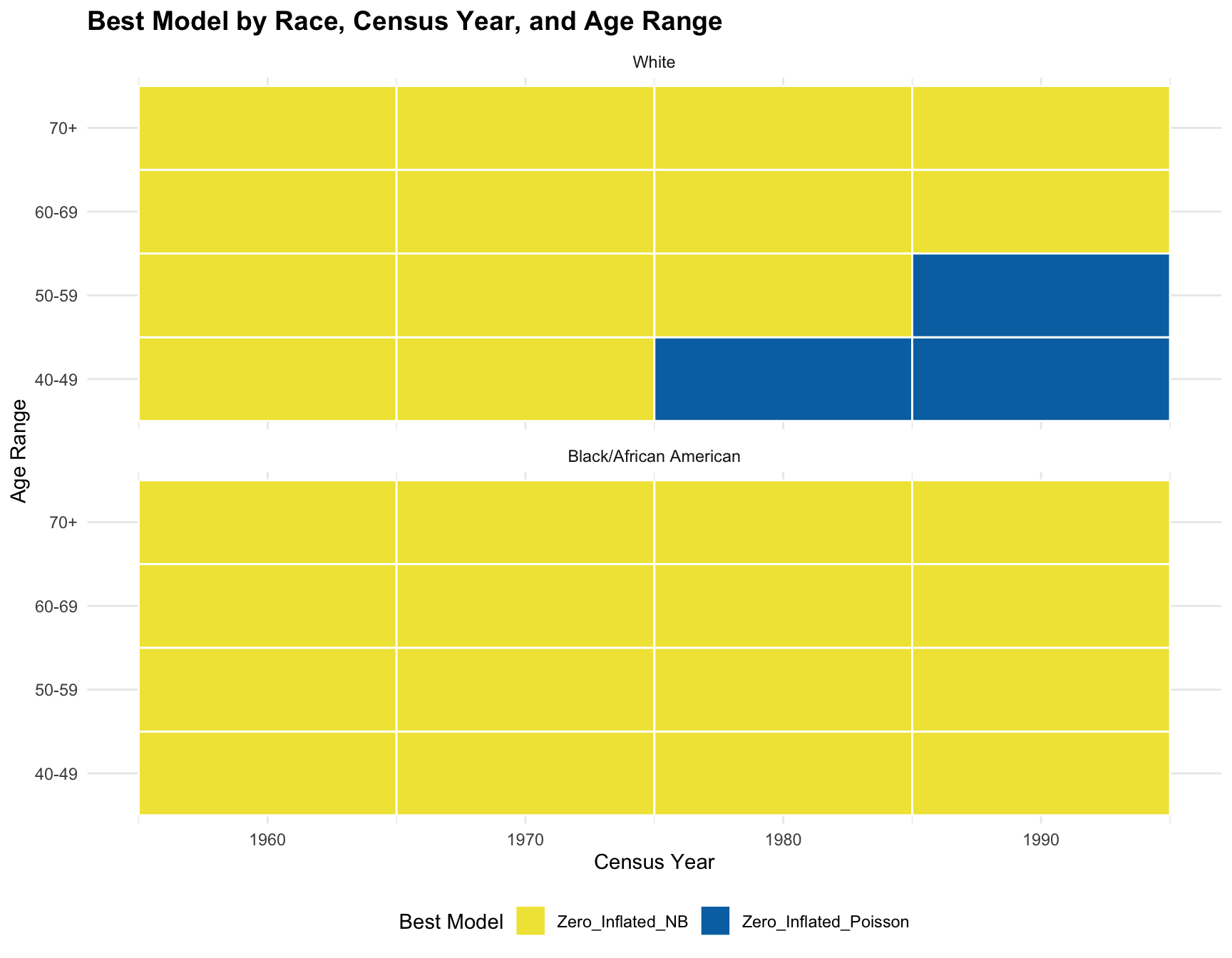
Conclusion:
- Best Model Analysis: The best-fitting model can be assessed across different races, census years, and age ranges by comparing models using AIC/BIC.
- Significance Testing: Use chi-square or logistic regression to assess which variable most influences the model selection.
- Summarizing Across Years: After analyzing the data, you’ll be able to conclude which model fits each race best across different years, and whether race, census year, or age group is the dominant factor.
CONCLUSION: The logistics regression shows that there isn’t a significant association between the predictors(races, age ranges, and census year) and the best-fitting model. According to the resulting visualization, the ZINB model is the best fit for the black population across census year and age group. However, the ZINB model perform the best among the white population only across year 1960 and 1970, and age group 60-69 and 70+.
[Instructions for Manqing] Cohort Stability Analysis
For Question 2: Cohort Stability Analysis, the goal is to determine if there is a significant change in zero inflation, family size, or model fit for the same cohort across different census years, given race.
Step 1: Add a Birth-Year “Cohort” Variable
Using the existing table of model summaries, calculate the birth-year cohort based on the Census Year and Age Range. For example, if a woman is in the 40-49 age range in the 1990 Census, her birth cohort would be 1941-1950.
- Formula to Calculate Cohort: For each row in the
table, subtract the age range from the census year to get the cohort.
For example:
- Census Year: 1990
- Age Range: 40-49
- Cohort: 1990 - (40 to 49) → Cohort: 1941-1950
- Add a new column to the summary table called
Cohort.
Example Table:
| Race | Census Year | Age Range | Best Model | Cohort |
|---|---|---|---|---|
| Black/African Am. | 1990 | 40-49 | Negative Binomial | 1941-1950 |
| White | 1990 | 40-49 | Zero-Inflated NB | 1941-1950 |
| White | 1980 | 50-59 | Poisson | 1921-1930 |
| … | … | … | … | … |
calculate_cohort <- function(census_year, age_range) {
  age_limits <- as.numeric(unlist(strsplit(age_range, "-|\\+")))

  if (length(age_limits) == 1) {
    lower_age <- age_limits
    upper_age <- Inf
  } else {
    lower_age <- age_limits[1]
    upper_age <- age_limits[2]
  }

  lower_cohort <- census_year - upper_age
  upper_cohort <- census_year - lower_age


  if (upper_age == Inf) {
    upper_cohort <- census_year - 70
  }

  return(paste(lower_cohort, upper_cohort, sep = "-"))
}

best_models <- best_models %>%
  mutate(Cohort = mapply(calculate_cohort, Census_Year, Age_Range)) %>%
  dplyr::select(Race, Census_Year, Age_Range, Best_Model, Cohort)

print(best_models)
Race Census_Year Age_Range Best_Model Cohort
1 White 1960 40-49 Zero_Inflated_NB 1911-1920
2 White 1960 50-59 Zero_Inflated_NB 1901-1910
3 White 1960 60-69 Zero_Inflated_NB 1891-1900
4 White 1960 70+ Zero_Inflated_NB -Inf-1890
5 Black/African American 1960 40-49 Zero_Inflated_NB 1911-1920
6 Black/African American 1960 50-59 Zero_Inflated_NB 1901-1910
7 Black/African American 1960 60-69 Zero_Inflated_NB 1891-1900
8 Black/African American 1960 70+ Zero_Inflated_NB -Inf-1890
9 White 1970 40-49 Zero_Inflated_NB 1921-1930
10 White 1970 50-59 Zero_Inflated_NB 1911-1920
11 White 1970 60-69 Zero_Inflated_NB 1901-1910
12 White 1970 70+ Zero_Inflated_NB -Inf-1900
13 Black/African American 1970 40-49 Zero_Inflated_NB 1921-1930
14 Black/African American 1970 50-59 Zero_Inflated_NB 1911-1920
15 Black/African American 1970 60-69 Zero_Inflated_NB 1901-1910
16 Black/African American 1970 70+ Zero_Inflated_NB -Inf-1900
17 White 1980 40-49 Zero_Inflated_Poisson 1931-1940
18 White 1980 50-59 Zero_Inflated_NB 1921-1930
19 White 1980 60-69 Zero_Inflated_NB 1911-1920
20 White 1980 70+ Zero_Inflated_NB -Inf-1910
21 Black/African American 1980 40-49 Zero_Inflated_NB 1931-1940
22 Black/African American 1980 50-59 Zero_Inflated_NB 1921-1930
23 Black/African American 1980 60-69 Zero_Inflated_NB 1911-1920
24 Black/African American 1980 70+ Zero_Inflated_NB -Inf-1910
25 White 1990 40-49 Zero_Inflated_Poisson 1941-1950
26 White 1990 50-59 Zero_Inflated_Poisson 1931-1940
27 White 1990 60-69 Zero_Inflated_NB 1921-1930
28 White 1990 70+ Zero_Inflated_NB -Inf-1920
29 Black/African American 1990 40-49 Zero_Inflated_NB 1941-1950
30 Black/African American 1990 50-59 Zero_Inflated_NB 1931-1940
31 Black/African American 1990 60-69 Zero_Inflated_NB 1921-1930
32 Black/African American 1990 70+ Zero_Inflated_NB -Inf-1920Step 2: Compute Summary Statistics for Each Subset
For each combination of Race, Cohort, and Census Year, compute additional summary statistics for family size distributions: - Mean, Variance, Mode of the number of children. - Probability of having 0, 1, 2, …, 12+ children (empirical or from the best-fitting model).
These statistics will help quantify family size changes over time.
Example Summary Table:
| Race | Cohort | Census Year | Best Model | Mean | Variance | Mode | Prob(0) | Prob(1) | Prob(2) | … | Prob(12+) |
|---|---|---|---|---|---|---|---|---|---|---|---|
| Black/African Am. | 1941-1950 | 1990 | Negative Binomial | 2.5 | 1.2 | 2 | 0.20 | 0.30 | 0.25 | … | 0.01 |
| White | 1941-1950 | 1990 | Zero-Inflated NB | 2.1 | 1.0 | 2 | 0.35 | 0.28 | 0.20 | … | 0.01 |
| White | 1921-1930 | 1980 | Poisson | 3.0 | 1.5 | 3 | 0.15 | 0.25 | 0.30 | … | 0.05 |
| … | … | … | … | … | … | … | … | … | … | … | … |
df_merg <- df %>%
  rename(Census_Year = YEAR, Race = RACE, Age_Range = AGE_RANGE)

# Perform a left join to merge the data frames
merged_data <- left_join(df_merg, best_models, by = c("Race", "Census_Year", "Age_Range"))
calculate_mode <- function(x) {
ux <- unique(x)
ux[which.max(tabulate(match(x, ux)))]
}
summary_table <- merged_data %>% group_by(Race, Cohort, Census_Year) %>%
summarise(
Mean = mean(chborn_num),
Variance = var(chborn_num),
Mode = calculate_mode(chborn_num),
Prob_0 = mean(chborn_num == 0),
Prob_1 = mean(chborn_num == 1),
Prob_2 = mean(chborn_num == 2),
Prob_3 = mean(chborn_num == 3),
Prob_4 = mean(chborn_num == 4),
Prob_5 = mean(chborn_num == 5),
Prob_6 = mean(chborn_num == 6),
Prob_7 = mean(chborn_num == 7),
Prob_8 = mean(chborn_num == 8),
Prob_9 = mean(chborn_num == 9),
Prob_10 = mean(chborn_num == 10),
Prob_11 = mean(chborn_num == 11),
Prob_12plus = mean(chborn_num >= 12)
#Total_Prob = Prob_0 + Prob_1 + Prob_2 + Prob_3 + Prob_4 + Prob_5 + Prob_6 +
# Prob_7 + Prob_8 + Prob_9 + Prob_10 + Prob_11 + Prob_12plus
) %>%
ungroup() %>% as.data.frame()`summarise()` has grouped output by 'Race', 'Cohort'. You can override using
the `.groups` argument.# View the summary table
print(summary_table) Race Cohort Census_Year Mean Variance Mode
1 White -Inf-1890 1960 3.295149 8.035775 2
2 White -Inf-1900 1970 2.619220 6.411794 0
3 White -Inf-1910 1980 2.259255 4.905316 0
4 White -Inf-1920 1990 2.310209 4.125397 2
5 White 1891-1900 1960 2.749532 6.109824 2
6 White 1901-1910 1960 2.357718 4.870047 2
7 White 1901-1910 1970 2.198574 4.786569 0
8 White 1911-1920 1960 2.383745 3.784971 2
9 White 1911-1920 1970 2.290355 3.947823 2
10 White 1911-1920 1980 2.299697 3.885418 2
11 White 1921-1930 1970 2.697188 3.906783 2
12 White 1921-1930 1980 2.728259 3.886124 2
13 White 1921-1930 1990 2.796851 3.950610 2
14 White 1931-1940 1980 2.901081 3.393930 2
15 White 1931-1940 1990 2.894691 3.351678 2
16 White 1941-1950 1990 2.204755 2.090623 2
17 Black/African American -Inf-1890 1960 3.902162 13.245048 0
18 Black/African American -Inf-1900 1970 3.087770 10.564482 0
19 Black/African American -Inf-1910 1980 2.613889 9.158011 0
20 Black/African American -Inf-1920 1990 2.856028 9.809749 0
21 Black/African American 1891-1900 1960 3.166572 10.973569 0
22 Black/African American 1901-1910 1960 2.741205 9.730068 0
23 Black/African American 1901-1910 1970 2.618036 9.023970 0
24 Black/African American 1911-1920 1960 2.820761 9.475099 0
25 Black/African American 1911-1920 1970 2.795064 9.124200 0
26 Black/African American 1911-1920 1980 2.817014 9.453284 0
27 Black/African American 1921-1930 1970 3.411675 9.564633 0
28 Black/African American 1921-1930 1980 3.400445 9.646242 0
29 Black/African American 1921-1930 1990 3.643816 10.234543 0
30 Black/African American 1931-1940 1980 3.721409 7.972764 3
31 Black/African American 1931-1940 1990 3.723892 7.741557 2
32 Black/African American 1941-1950 1990 2.690402 3.955388 2
Prob_0 Prob_1 Prob_2 Prob_3 Prob_4 Prob_5 Prob_6
1 0.1601171 0.14383842 0.1735320 0.14095304 0.10820180 0.07719472 0.05585582
2 0.2337344 0.15563563 0.1907270 0.13766146 0.09400089 0.06100962 0.04147614
3 0.2425410 0.17905944 0.2217025 0.14213617 0.08185637 0.04957835 0.03016161
4 0.2003224 0.17086054 0.2495743 0.16517318 0.09503183 0.05020253 0.02764322
5 0.1790942 0.17183505 0.2064320 0.14997168 0.10013557 0.06473203 0.04249112
6 0.2000759 0.19774610 0.2351671 0.14591432 0.08571877 0.04872973 0.03009123
7 0.2484123 0.18579166 0.2226615 0.13859746 0.08031093 0.04560480 0.02848213
8 0.1548323 0.18555184 0.2691760 0.17613893 0.09801059 0.05041189 0.02763336
9 0.1967171 0.16973904 0.2562944 0.16982255 0.09505741 0.04905532 0.02524530
10 0.1926550 0.16842906 0.2583952 0.17291618 0.09513579 0.04901138 0.02691150
11 0.1351880 0.12673286 0.2507330 0.20721415 0.13102862 0.06863779 0.03679984
12 0.1318459 0.12042477 0.2503092 0.21324354 0.13229042 0.07044023 0.03706567
13 0.1234195 0.11569770 0.2477657 0.21626065 0.13752802 0.07369103 0.03953569
14 0.1037357 0.09351712 0.2399871 0.23964134 0.16043259 0.08265468 0.04216199
15 0.1031027 0.09122701 0.2441949 0.24135347 0.15966028 0.08278604 0.04035221
16 0.1389518 0.13595406 0.3532313 0.22043189 0.09474345 0.03452663 0.01315010
17 0.1979522 0.14761092 0.1242890 0.08902162 0.08447099 0.05830489 0.06058020
18 0.2601452 0.16502234 0.1285369 0.09959047 0.08460536 0.05835815 0.04579300
19 0.3019568 0.19414247 0.1310909 0.09464126 0.06778360 0.04744852 0.03824018
20 0.2758865 0.18308004 0.1298886 0.09979737 0.07163121 0.05420466 0.04346505
21 0.2480664 0.17732503 0.1284663 0.09677419 0.07508017 0.05715903 0.04584041
22 0.2864718 0.19580962 0.1319193 0.09169684 0.07281428 0.04837041 0.03879979
23 0.2998207 0.18659938 0.1367953 0.09436218 0.07231556 0.05491733 0.03625739
24 0.2685870 0.18750000 0.1383696 0.09891304 0.07510870 0.05206522 0.04413043
25 0.2644968 0.18741749 0.1396872 0.10373718 0.07936427 0.05255408 0.04305880
26 0.2708013 0.17914380 0.1436883 0.10406147 0.07178924 0.05433589 0.04368825
27 0.1825328 0.15683751 0.1417145 0.12075385 0.09643760 0.07621236 0.05796369
28 0.1890040 0.15089492 0.1437869 0.12280552 0.09454483 0.07185065 0.05917616
29 0.1674815 0.14605222 0.1425153 0.11640487 0.09497555 0.07968376 0.06407989
30 0.1190148 0.12667930 0.1436445 0.14424733 0.12435412 0.10032725 0.07543920
31 0.1110096 0.12261307 0.1537688 0.14536318 0.13001370 0.09821836 0.07747830
32 0.1258126 0.15923518 0.2409178 0.18860421 0.12466539 0.07319312 0.04221797
Prob_7 Prob_8 Prob_9 Prob_10 Prob_11 Prob_12plus
1 0.041084387 0.034021662 0.0232983786 0.0170538963 0.0107017506 0.0141469822
2 0.027730366 0.021085755 0.0136685140 0.0098475111 0.0061248428 0.0072978345
3 0.018016649 0.012731042 0.0087478429 0.0054809686 0.0032668743 0.0047212303
4 0.015665041 0.009936348 0.0059849549 0.0041084566 0.0023807556 0.0031164752
5 0.028642035 0.019752536 0.0133514098 0.0101079439 0.0054400988 0.0080142781
6 0.019685606 0.013481499 0.0084292090 0.0063219068 0.0035732517 0.0050653787
7 0.016949039 0.011846964 0.0078935242 0.0056162892 0.0031186767 0.0047147446
8 0.015027420 0.008985590 0.0057688199 0.0033710799 0.0022909100 0.0028013199
9 0.014739040 0.009003132 0.0055114823 0.0034551148 0.0020929019 0.0032672234
10 0.013830609 0.009086128 0.0053711101 0.0032338559 0.0018127497 0.0032114763
11 0.018971640 0.010663352 0.0060738619 0.0036086503 0.0017938349 0.0025543789
12 0.019924245 0.010812430 0.0055849728 0.0036524562 0.0019035288 0.0025026089
13 0.019747920 0.011179196 0.0063567977 0.0038260350 0.0019827629 0.0030090171
14 0.019447458 0.009181204 0.0046502200 0.0023370336 0.0011565932 0.0010969750
15 0.019026010 0.009492189 0.0043714027 0.0021336608 0.0010720345 0.0012281560
16 0.005115379 0.002117610 0.0008191578 0.0004008645 0.0002875767 0.0002701478
17 0.047781570 0.044368601 0.0346985210 0.0315699659 0.0236063709 0.0557451650
18 0.037043931 0.029318690 0.0252233805 0.0209419211 0.0134028295 0.0320178704
19 0.034531270 0.023404527 0.0170098478 0.0170098478 0.0092083387 0.0235324210
20 0.037082067 0.029078014 0.0217831814 0.0163120567 0.0094224924 0.0283687943
21 0.039615167 0.034899076 0.0239577438 0.0260328240 0.0130164120 0.0337672137
22 0.029487843 0.028711847 0.0210812209 0.0165545784 0.0102172788 0.0280651837
23 0.029749651 0.023109104 0.0184607212 0.0138787436 0.0094959825 0.0242379972
24 0.035434783 0.026847826 0.0191304348 0.0186956522 0.0103260870 0.0248913043
25 0.031938662 0.028688941 0.0201076470 0.0160454961 0.0108662537 0.0220371687
26 0.031503842 0.025795829 0.0222832053 0.0171240395 0.0107574094 0.0250274424
27 0.049046196 0.036037692 0.0242702827 0.0204091014 0.0130085038 0.0247759136
28 0.047529331 0.036139419 0.0262053610 0.0196968399 0.0139590648 0.0244069538
29 0.052637054 0.039633829 0.0263185270 0.0241339852 0.0160199730 0.0300634557
30 0.057698932 0.040475370 0.0259214606 0.0170513262 0.0102480193 0.0148983810
31 0.055824577 0.039013248 0.0278666058 0.0152581087 0.0074920055 0.0160804020
32 0.020573614 0.012848948 0.0061185468 0.0022944551 0.0014531549 0.0020650096Step 3: Test for Significant Changes Over Time Within Each Cohort
Once the cohort information and summary statistics are available, the goal is to determine if there is a significant change in any of the following across census years for the same cohort:
- Zero Inflation: Check if the proportion of women with zero children changes significantly over time for the same cohort.
- Family Size: Test if the mean or variance in the number of children changes for the same cohort over time.
- Model Fit: Analyze if the best-fitting model for the cohort changes over time.
a. Zero-Inflation Analysis
Use a logistic regression model to assess if the probability of having zero children changes significantly over time for the same cohort.
Example Code:
## divided the corhort by race
merged_df_black <- merged_data %>% filter(Race == "Black/African American")
merged_df_white <- merged_data %>% filter(Race == "White")
# Filter cohorts with more than one census year
cohort_counts <- merged_df_black %>%
group_by(Cohort) %>%
summarise(Unique_Census_Years = n_distinct(Census_Year)) %>%
filter(Unique_Census_Years > 1)
# Get the list of cohorts for testing
cohorts_for_test <- cohort_counts$Cohort
# Initialize results data frame
results_black <- data.frame(RACE = character(), Cohort = character(), Chi_Square = numeric(), p_value = numeric(), stringsAsFactors = FALSE)
# Loop through each cohort and run the chi-square test
for (cohort in cohorts_for_test) {
cohort_data <- merged_df_black %>% filter(Cohort == cohort)
# Create contingency table
contingency_table <- table(cohort_data$Census_Year, cohort_data$chborn_num == "0")
# Perform the chi-square test only if more than one row is in the table
if (nrow(contingency_table) > 1) {
test_result <- chisq.test(contingency_table)
# Append results to the results data frame
results_black <- rbind(results_black, data.frame(
RACE = "Black/African American",
Cohort = cohort,
Chi_Square = test_result$statistic,
p_value = test_result$p.value
))
}
}
results_black <- results_black %>%
mutate(Significance = ifelse(p_value > 0.05, "No", "Yes"))
print(results_black) RACE Cohort Chi_Square p_value
X-squared Black/African American 1901-1910 4.310851 0.0378700083
X-squared1 Black/African American 1911-1920 1.421550 0.4912633533
X-squared2 Black/African American 1921-1930 17.245995 0.0001799202
X-squared3 Black/African American 1931-1940 3.466056 0.0626405054
Significance
X-squared Yes
X-squared1 No
X-squared2 Yes
X-squared3 No# Filter cohorts with more than one census year
cohort_counts2 <- merged_df_white %>%
group_by(Cohort) %>%
summarise(Unique_Census_Years = n_distinct(Census_Year)) %>%
filter(Unique_Census_Years > 1)
# Get the list of cohorts for testing
cohorts_for_test2 <- cohort_counts2$Cohort
# Initialize results data frame
results_white <- data.frame(RACE = character(), Cohort = character(), Chi_Square = numeric(), p_value = numeric(), stringsAsFactors = FALSE)
# Loop through each cohort and run the chi-square test
for (cohort in cohorts_for_test2) {
cohort_data <- merged_df_white %>% filter(Cohort == cohort)
# Create contingency table
contingency_table <- table(cohort_data$Census_Year, cohort_data$chborn_num == "0")
# Perform the chi-square test only if more than one row is in the table
if (nrow(contingency_table) > 1) {
test_result <- chisq.test(contingency_table)
# Append results to the results data frame
results_white <- rbind(results_white, data.frame(
RACE = "White",
Cohort = cohort,
Chi_Square = test_result$statistic,
p_value = test_result$p.value
))
}
}
results_white <- results_white %>%
mutate(Significance = ifelse(p_value > 0.05, "No", "Yes"))
print(results_white) RACE Cohort Chi_Square p_value Significance
X-squared White 1901-1910 662.9400598 3.427247e-146 Yes
X-squared1 White 1911-1920 711.8344845 2.673657e-155 Yes
X-squared2 White 1921-1930 80.1733778 3.895581e-18 Yes
X-squared3 White 1931-1940 0.1867867 6.656046e-01 No# Combine the two data frames
combined_result <- rbind(results_black, results_white)
# Create the plot
ggplot(combined_result, aes(x = Cohort, y = p_value, color = RACE, shape = Significance)) +
geom_point(size = 2) +
geom_line(aes(group = RACE)) +
annotate("text", x = Inf, y = 0.05, label = "p = 0.05", hjust = 1.1, vjust = -0.5, color = "red", size = 3) +
geom_hline(yintercept = 0.05, linetype = "dashed", color = "red", size = 0.5) +
scale_y_log10() + # Use log scale for better visualization if p-values vary widely
labs(
title = "Change of p-values by Cohort",
x = "Cohort",
y = "p-value (log scale)",
color = "Race",
shape = "Significance"
) +
theme_minimal() +
theme(axis.text.x = element_text(angle = 45, hjust = 1))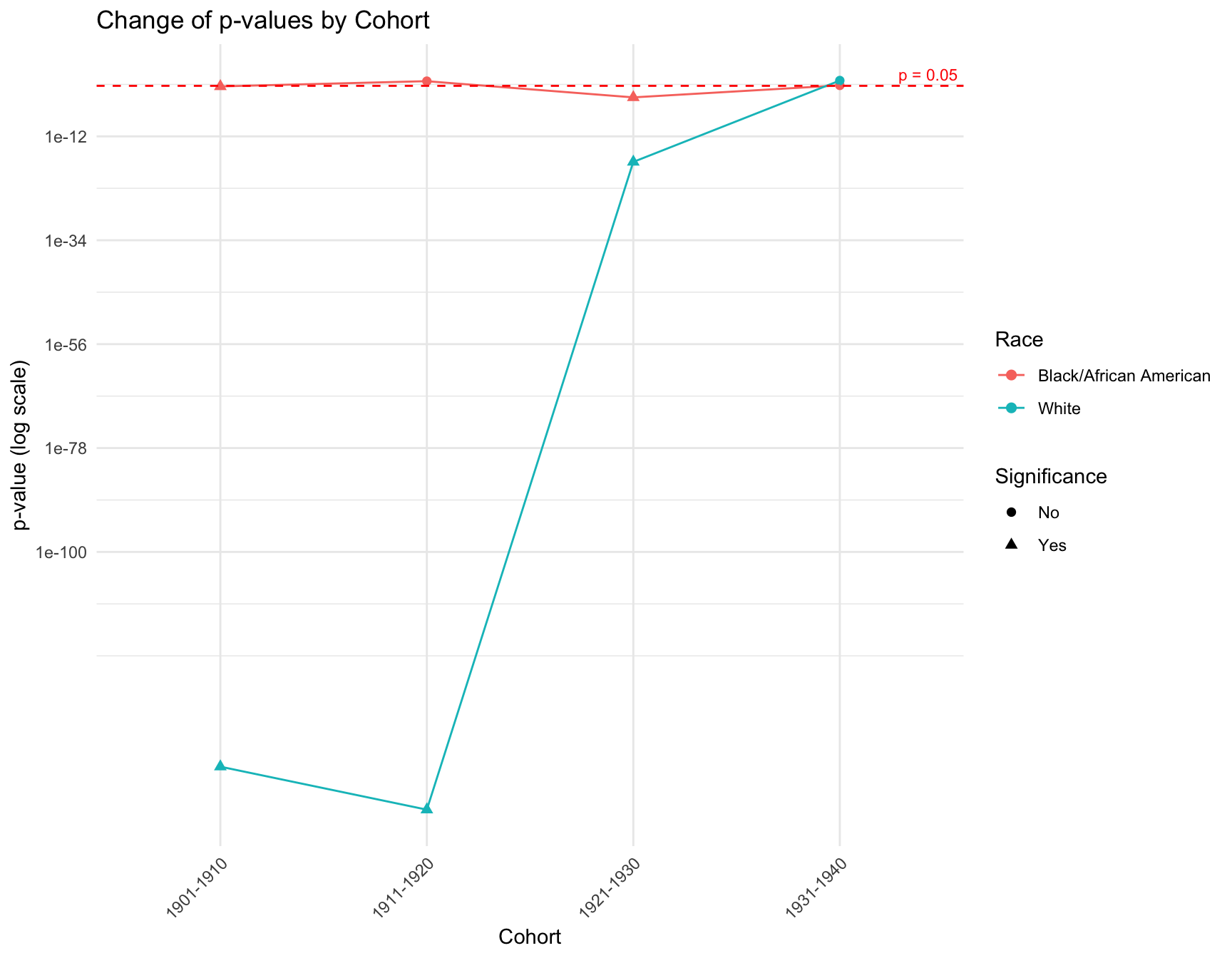
| Version | Author | Date |
|---|---|---|
| 2851385 | Tina Lasisi | 2024-09-21 |
RESULT: The graph shows that there is a discrepancy in the p-value within the cohorts like 1901-1910, 1911-1920 and 1921-1930 by race. However, in cohort 1931-1941, the p-value of each race is pretty close to each other. The overall trend of the p-value for black population is stable across cohort, while the trend for white population fluctuate a lot.
ggplot(combined_result, aes(x = Cohort, y = Chi_Square, color = RACE)) +
  geom_point(size = 3) +
  geom_line(aes(group = RACE)) +
  labs(
    title = "Change of Test Statistics by Cohort",
    x = "Cohort",
    y = "Chi-Square",
    color = "Race"
  ) +
  theme_minimal() +
  theme(axis.text.x = element_text(angle = 45, hjust = 1))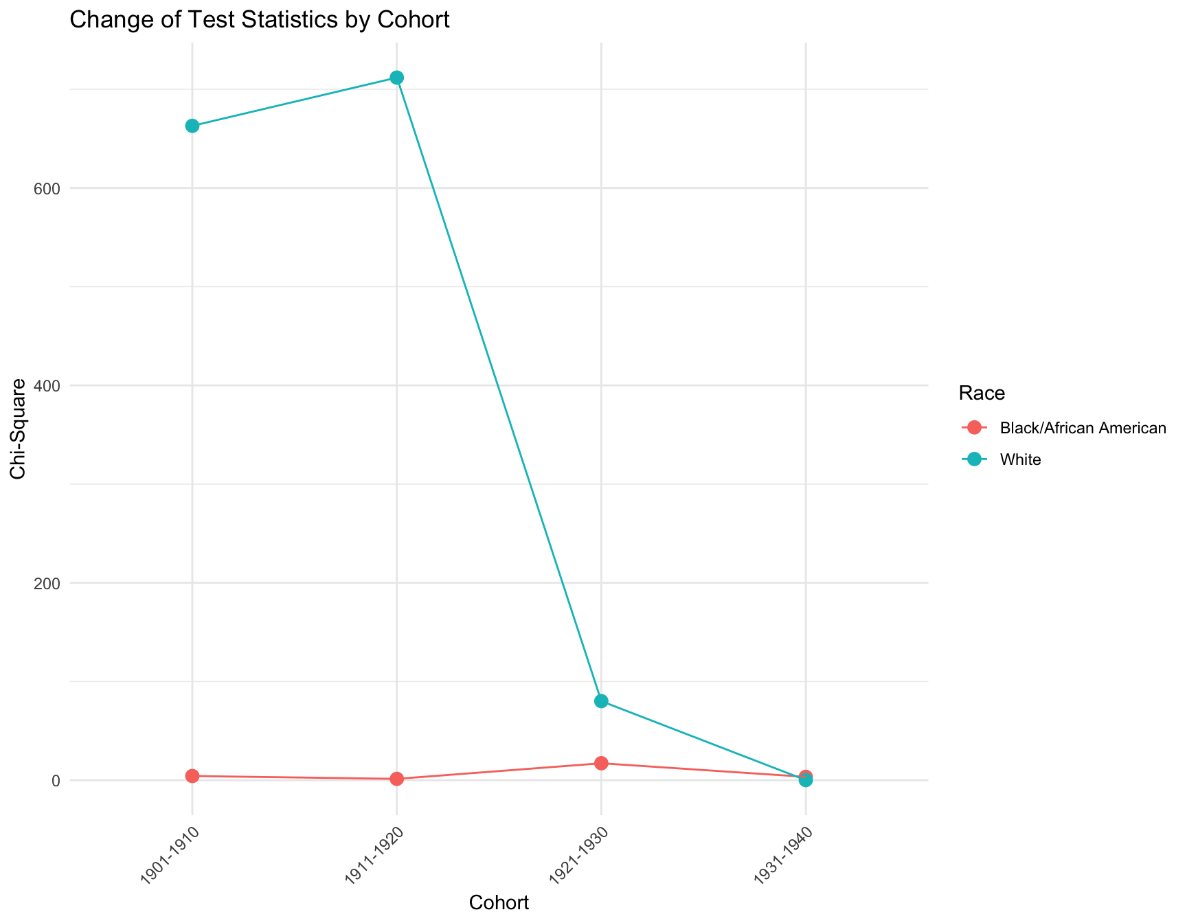
| Version | Author | Date |
|---|---|---|
| 2851385 | Tina Lasisi | 2024-09-21 |
CONCLUSION: We observe that the proportion of women with zero children change significantly across census year in the following cohort by race: -black population:1901-1910, 1921-1930 -white population:1901-1910, 1911-1920, 1921-1930
b. Family Size Analysis
Use an ANOVA or linear regression to test if the mean or variance in family size changes over census years for the same cohort.
Example Code:
  # Fit linear model to check for changes in family size over time
  #family_size_model <- lm(Mean ~ Census_Year, data = summary_table)

  # ANOVA to check for significant differences in mean
  #anova(family_size_model)
merged_data2 <- left_join(merged_data, summary_table, by = c("Race","Cohort","Census_Year")) %>% dplyr::select(Race, Cohort, Census_Year, Mean, Variance)
merged_black = merged_data2 %>% filter(Race == "Black/African American")
merged_white = merged_data2 %>% filter(Race == "White")cohorts1 <- unique(merged_black$Cohort)
# Loop through each cohort and apply ANOVA for Mean and Variance
for (cohort in cohorts1) {
# Filter data for the specific cohort
cohort_data_b <- merged_black[merged_black$Cohort == cohort, ]
# Check if there are at least two unique Census_Year values
if (length(unique(cohort_data_b$Census_Year)) < 2) {
cat("\nCohort:", cohort, "has only one Census Year. Skipping ANOVA.\n")
next
}
# Perform ANOVA for Mean
anova_mean_result <- aov(Mean ~ factor(Census_Year), data = cohort_data_b)
# Perform ANOVA for Variance
anova_variance_result <- aov(Variance ~ factor(Census_Year), data = cohort_data_b)
# Output the results
cat("\nCohort:", cohort)
cat("\nANOVA for Mean Family Size:\n")
print(summary(anova_mean_result))
cat("\nANOVA for Variance in Family Size:\n")
print(summary(anova_variance_result))
}
Cohort: 1891-1900 has only one Census Year. Skipping ANOVA.

Cohort: 1911-1920
ANOVA for Mean Family Size:
                       Df Sum Sq Mean Sq   F value Pr(>F)
factor(Census_Year)     2  5.453   2.727 8.507e+23 <2e-16 ***
Residuals           38001  0.000   0.000
---
Signif. codes:  0 '***' 0.001 '**' 0.01 '*' 0.05 '.' 0.1 ' ' 1

ANOVA for Variance in Family Size:
                       Df Sum Sq Mean Sq   F value Pr(>F)
factor(Census_Year)     2   1099   549.7 7.821e+25 <2e-16 ***
Residuals           38001      0     0.0
---
Signif. codes:  0 '***' 0.001 '**' 0.01 '*' 0.05 '.' 0.1 ' ' 1

Cohort: 1901-1910
ANOVA for Mean Family Size:
                       Df Sum Sq Mean Sq   F value Pr(>F)
factor(Census_Year)     1  77.51   77.51 7.094e+25 <2e-16 ***
Residuals           22789   0.00    0.00
---
Signif. codes:  0 '***' 0.001 '**' 0.01 '*' 0.05 '.' 0.1 ' ' 1

ANOVA for Variance in Family Size:
                       Df Sum Sq Mean Sq   F value Pr(>F)
factor(Census_Year)     1   2547    2547 8.424e+26 <2e-16 ***
Residuals           22789      0       0
---
Signif. codes:  0 '***' 0.001 '**' 0.01 '*' 0.05 '.' 0.1 ' ' 1

Cohort: -Inf-1890 has only one Census Year. Skipping ANOVA.

Cohort: 1921-1930
ANOVA for Mean Family Size:
                       Df Sum Sq Mean Sq   F value Pr(>F)
factor(Census_Year)     2    417   208.5 4.477e+26 <2e-16 ***
Residuals           43042      0     0.0
---
Signif. codes:  0 '***' 0.001 '**' 0.01 '*' 0.05 '.' 0.1 ' ' 1

ANOVA for Variance in Family Size:
                       Df Sum Sq Mean Sq   F value Pr(>F)
factor(Census_Year)     2   3122    1561 4.647e+25 <2e-16 ***
Residuals           43042      0       0
---
Signif. codes:  0 '***' 0.001 '**' 0.01 '*' 0.05 '.' 0.1 ' ' 1

Cohort: -Inf-1900 has only one Census Year. Skipping ANOVA.

Cohort: 1931-1940
ANOVA for Mean Family Size:
                       Df  Sum Sq Mean Sq   F value Pr(>F)
factor(Census_Year)     1 0.03475 0.03475 1.223e+22 <2e-16 ***
Residuals           22555 0.00000 0.00000
---
Signif. codes:  0 '***' 0.001 '**' 0.01 '*' 0.05 '.' 0.1 ' ' 1

ANOVA for Variance in Family Size:
                       Df Sum Sq Mean Sq  F value Pr(>F)
factor(Census_Year)     1  301.2   301.2 6.73e+25 <2e-16 ***
Residuals           22555    0.0     0.0
---
Signif. codes:  0 '***' 0.001 '**' 0.01 '*' 0.05 '.' 0.1 ' ' 1

Cohort: -Inf-1910 has only one Census Year. Skipping ANOVA.

Cohort: 1941-1950 has only one Census Year. Skipping ANOVA.

Cohort: -Inf-1920 has only one Census Year. Skipping ANOVA.
cohorts2 <- unique(merged_white$Cohort)
# Loop through each cohort and apply ANOVA for Mean and Variance
for (cohort in cohorts2) {
# Filter data for the specific cohort
cohort_data_w <- merged_white[merged_white$Cohort == cohort, ]
# Check if there are at least two unique Census_Year values
if (length(unique(cohort_data_w$Census_Year)) < 2) {
cat("\nCohort:", cohort, "has only one Census Year. Skipping ANOVA.\n")
next
}
# Perform ANOVA for Mean
anova_mean_result <- aov(Mean ~ factor(Census_Year), data = cohort_data_w)
# Perform ANOVA for Variance
anova_variance_result <- aov(Variance ~ factor(Census_Year), data = cohort_data_w)
# Output the results
cat("\nCohort:", cohort)
cat("\nANOVA for Mean Family Size:\n")
print(summary(anova_mean_result))
cat("\nANOVA for Variance in Family Size:\n")
print(summary(anova_variance_result))
}
Cohort: 1891-1900 has only one Census Year. Skipping ANOVA.

Cohort: 1911-1920
ANOVA for Mean Family Size:
                        Df Sum Sq Mean Sq   F value Pr(>F)
factor(Census_Year)      2  535.2   267.6 4.546e+24 <2e-16 ***
Residuals           365210    0.0     0.0
---
Signif. codes:  0 '***' 0.001 '**' 0.01 '*' 0.05 '.' 0.1 ' ' 1

ANOVA for Variance in Family Size:
                        Df Sum Sq Mean Sq   F value Pr(>F)
factor(Census_Year)      2   1563   781.4 4.723e+25 <2e-16 ***
Residuals           365210      0     0.0
---
Signif. codes:  0 '***' 0.001 '**' 0.01 '*' 0.05 '.' 0.1 ' ' 1

Cohort: 1901-1910
ANOVA for Mean Family Size:
                        Df Sum Sq Mean Sq   F value Pr(>F)
factor(Census_Year)      1   1281    1281 9.604e+25 <2e-16 ***
Residuals           226142      0       0
---
Signif. codes:  0 '***' 0.001 '**' 0.01 '*' 0.05 '.' 0.1 ' ' 1

ANOVA for Variance in Family Size:
                        Df Sum Sq Mean Sq   F value Pr(>F)
factor(Census_Year)      1  352.5   352.5 6.248e+23 <2e-16 ***
Residuals           226142    0.0     0.0
---
Signif. codes:  0 '***' 0.001 '**' 0.01 '*' 0.05 '.' 0.1 ' ' 1

Cohort: -Inf-1890 has only one Census Year. Skipping ANOVA.

Cohort: -Inf-1900 has only one Census Year. Skipping ANOVA.

Cohort: 1921-1930
ANOVA for Mean Family Size:
                        Df Sum Sq Mean Sq   F value Pr(>F)
factor(Census_Year)      2  653.9     327 8.029e+23 <2e-16 ***
Residuals           394507    0.0       0
---
Signif. codes:  0 '***' 0.001 '**' 0.01 '*' 0.05 '.' 0.1 ' ' 1

ANOVA for Variance in Family Size:
                        Df Sum Sq Mean Sq   F value Pr(>F)
factor(Census_Year)      2    224     112 2.455e+24 <2e-16 ***
Residuals           394507      0       0
---
Signif. codes:  0 '***' 0.001 '**' 0.01 '*' 0.05 '.' 0.1 ' ' 1

Cohort: 1931-1940
ANOVA for Mean Family Size:
                        Df Sum Sq Mean Sq   F value Pr(>F)
factor(Census_Year)      1  1.829   1.829 8.533e+22 <2e-16 ***
Residuals           179944  0.000   0.000
---
Signif. codes:  0 '***' 0.001 '**' 0.01 '*' 0.05 '.' 0.1 ' ' 1

ANOVA for Variance in Family Size:
                        Df Sum Sq Mean Sq   F value Pr(>F)
factor(Census_Year)      1  79.94   79.94 1.017e+24 <2e-16 ***
Residuals           179944   0.00    0.00
---
Signif. codes:  0 '***' 0.001 '**' 0.01 '*' 0.05 '.' 0.1 ' ' 1

Cohort: -Inf-1910 has only one Census Year. Skipping ANOVA.

Cohort: -Inf-1920 has only one Census Year. Skipping ANOVA.

Cohort: 1941-1950 has only one Census Year. Skipping ANOVA.
RESULT: 1.In both racial group, the ANOVA is not applicable for the following cohort since there is only one census year available in the data for those cohorts:-Inf-1910, 1941-1950, -Inf-1920, -Inf-1890, -Inf-1900, and 1891-1900 2.By looking at the ANOVA for mean and variance family size in both racial group, the p-value of the rest cohorts (1901-1910, 1911-1920, 1921-1930, 1931-1940) are smaller than 0.05, indicating mean and variance family size for these cohort has significantly changed over different census years in both population.
c. Model Fit Analysis
- If the best-fitting model changes for the same cohort over time, this suggests that the distribution of family sizes has shifted. Use multinomial logistic regression to test if the model fit differs across census years for the same cohort.
Example Code:
# Test for white population
test_df_w <- merged_data %>%
  mutate(Best_Model_Binary = ifelse(Best_Model == "Zero_Inflated_NB", 1, 0)) %>%
  select(Race, Cohort, Census_Year, Best_Model, Best_Model_Binary) %>%
  filter(Race == "White")

unique_cohorts <- unique(test_df_w$Cohort)

for (cohort in unique_cohorts) {
  cohort_data <- test_df_w %>% filter(Cohort == cohort)

  if (n_distinct(cohort_data$Census_Year) > 1) {
    if (n_distinct(cohort_data$Best_Model_Binary) > 1) {
      logistic_model <- glm(Best_Model_Binary ~ as.factor(Census_Year), data = cohort_data, family = binomial)

      print(paste("Cohort:", cohort))
      print(summary(logistic_model))
    } else {
      print(paste("Warning for Cohort", cohort, ": Best_Model_Binary contains only a single category. Model convergence issues likely due to lack of variability."))
    }
  } else {
    print(paste("Cohort:", cohort, "- Not enough data variability across census years for logistic regression."))
  }
}
[1] "Cohort: 1891-1900 - Not enough data variability across census years for logistic regression."
[1] "Warning for Cohort 1911-1920 : Best_Model_Binary contains only a single category. Model convergence issues likely due to lack of variability."
[1] "Warning for Cohort 1901-1910 : Best_Model_Binary contains only a single category. Model convergence issues likely due to lack of variability."
[1] "Cohort: -Inf-1890 - Not enough data variability across census years for logistic regression."
[1] "Cohort: -Inf-1900 - Not enough data variability across census years for logistic regression."
[1] "Warning for Cohort 1921-1930 : Best_Model_Binary contains only a single category. Model convergence issues likely due to lack of variability."
[1] "Warning for Cohort 1931-1940 : Best_Model_Binary contains only a single category. Model convergence issues likely due to lack of variability."
[1] "Cohort: -Inf-1910 - Not enough data variability across census years for logistic regression."
[1] "Cohort: -Inf-1920 - Not enough data variability across census years for logistic regression."
[1] "Cohort: 1941-1950 - Not enough data variability across census years for logistic regression."# Test for black population
test_df_b <- merged_data %>%
mutate(Best_Model_Binary = ifelse(Best_Model == "Zero_Inflated_NB", 1, 0)) %>%
select(Race, Cohort, Census_Year, Best_Model, Best_Model_Binary) %>%
filter(Race == "Black/African American")
unique_cohorts <- unique(test_df_b$Cohort)
for (cohort in unique_cohorts) {
cohort_data <- test_df_b %>% filter(Cohort == cohort)
if (n_distinct(cohort_data$Census_Year) > 1) {
if (n_distinct(cohort_data$Best_Model_Binary) > 1) {
logistic_model <- glm(Best_Model_Binary ~ as.factor(Census_Year), data = cohort_data, family = binomial)
print(paste("Cohort:", cohort))
print(summary(logistic_model))
} else {
print(paste("Warning for Cohort", cohort, ": Best_Model_Binary contains only a single category. Model convergence issues likely due to lack of variability."))
}
} else {
print(paste("Cohort:", cohort, "- Not enough data variability across census years for logistic regression."))
}
}[1] "Cohort: 1891-1900 - Not enough data variability across census years for logistic regression."
[1] "Warning for Cohort 1911-1920 : Best_Model_Binary contains only a single category. Model convergence issues likely due to lack of variability."
[1] "Warning for Cohort 1901-1910 : Best_Model_Binary contains only a single category. Model convergence issues likely due to lack of variability."
[1] "Cohort: -Inf-1890 - Not enough data variability across census years for logistic regression."
[1] "Warning for Cohort 1921-1930 : Best_Model_Binary contains only a single category. Model convergence issues likely due to lack of variability."
[1] "Cohort: -Inf-1900 - Not enough data variability across census years for logistic regression."
[1] "Warning for Cohort 1931-1940 : Best_Model_Binary contains only a single category. Model convergence issues likely due to lack of variability."
[1] "Cohort: -Inf-1910 - Not enough data variability across census years for logistic regression."
[1] "Cohort: 1941-1950 - Not enough data variability across census years for logistic regression."
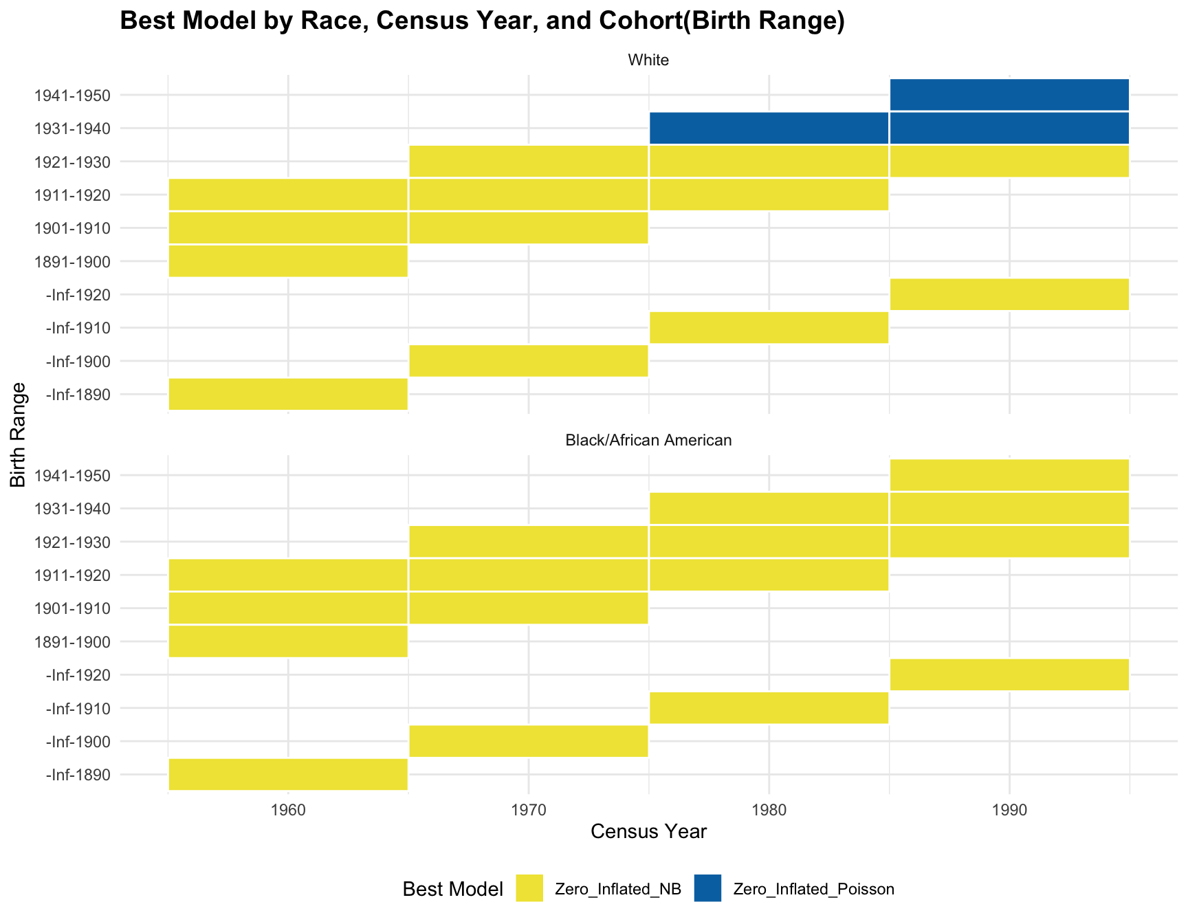
[1] "Cohort: -Inf-1920 - Not enough data variability across census years for logistic regression."# Due to the problem indicated above, I use an alternative method:visualization
ggplot(best_models, aes(x = Census_Year, y = Cohort, fill = Best_Model)) +
geom_tile(color = "white", lwd = 0.5, linetype = 1) + # Create the tiles
facet_wrap(~Race, nrow = 2) + # Facet by Race
scale_fill_manual(values = c("Zero_Inflated_Poisson" = "#0072B2", "Zero_Inflated_NB" = "#F0E442")) +
labs(
title = "Best Model by Race, Census Year, and Cohort(Birth Range)",
x = "Census Year",
y = "Birth Range",
fill = "Best Model"
) +
theme_minimal() +
theme(
plot.title = element_text(size = 14, face = "bold"),
legend.position = "bottom"
)
| Version | Author | Date |
|---|---|---|
| 2851385 | Tina Lasisi | 2024-09-21 |
RESULT: Based on the heatmap created, we can see that the model fit for each cohort across year does not change.
Step 4: Interpret the Results
For each cohort, you will assess whether: - Zero-inflation changes significantly over time (i.e., whether the probability of having no children decreases or increases across census years). - Family size (mean, variance, mode) changes significantly over time. - The best-fitting model changes over time, indicating a shift in family size distributions.
If significant changes are detected for a cohort (e.g., the same cohort switches from a zero-inflated model to a non-zero-inflated model, or family sizes decrease), this indicates a shift in the demographic pattern for that group.
Conclusion
This analysis will allow you to evaluate cohort stability by testing whether demographic patterns (e.g., zero-inflation, family size) are consistent over time for the same cohort or if there are notable shifts. If the patterns change significantly, you will be able to identify when and how the demographic trends for each cohort begin to deviate from their earlier distribution.
[Instructions for Manqing] Question 3: Analyzing and Visualizing Significant Fertility Shifts
For Question 3: Significant Fertility shifts, the goal is to summarize the information in the top 2 questions and create a comprehensive analysis and visualization that illustrates significant fertility shifts in cohorts, compares fertility patterns of 40-49 year-olds to 50-59 year-olds in the 1990 census so we can pick the set of fertility distributions we want to use to visualize the sibling distribution and do the math on the genetic surveillance.
Objective
Create a comprehensive analysis and visualization that:
- Illustrates significant fertility shifts in cohorts based on the stability analysis from Question 2.
- Compares fertility patterns of 40-49 year-olds to 50-59 year-olds in the 1990 census, highlighting any significant differences.
- Synthesizes the findings to discuss overall trends and their implications.
The steps below are suggestions: use critical thinking and your judgement to complete this task and answer the question
Step 1: Prepare the Data
1.1 Use Results from Stability Analysis (Question 2)
- Identify Cohorts with Significant Shifts:
- Review the results from your stability analysis in Question 2.
- List the cohorts where significant shifts in fertility distributions were observed for 40-49 year-olds.
- Note the nature of these shifts for each cohort, such as changes in mean number of children, variance, or zero inflation (proportion of women with zero children).
1.2 Extract Data for Age Groups in 1990 Census
- Filter Data for 1990 Census:
- Use your existing dataset to extract data specifically from the 1990 census year.
- Select Age Groups:
- Focus on women in the age ranges of 40-49 and 50-59.
- Ensure the data includes necessary variables:
- Number of children (
chborn_num) - Age range (
AGE_RANGE) - Race (
RACE) - Any other relevant variables used in previous analyses
- Number of children (
Step 2: Create Visualizations
Design visualizations that effectively communicate your findings.
2.1 Panel A: Fertility Distribution Shifts Across Cohorts
- Use Existing Fertility Distribution Plots:
- Leverage the fertility distribution plots you created in Question 1.
- Highlight Significant Cohorts:
- Emphasize the cohorts identified in Step 1.1 where significant
shifts occurred.
- This could be done by using distinct colors, markers, or annotations.
- Emphasize the cohorts identified in Step 1.1 where significant
shifts occurred.
- Annotate the Plots:
- Include text or labels that describe the nature of the significant
shifts for each highlighted cohort.
- For example, indicate if there was a decrease in mean number of children or an increase in childlessness.
- Include text or labels that describe the nature of the significant
shifts for each highlighted cohort.
part1<- child_plot +
  geom_rect(data = df_mirror %>% filter((YEAR == 1960 & AGE_RANGE == "50-59")|
                                        (YEAR == 1970 & AGE_RANGE == "40-49")|
                                        (YEAR == 1970 & AGE_RANGE == "60-69")|
                                        (YEAR == 1980 & AGE_RANGE == "50-59")|
                                        (YEAR == 1990 & AGE_RANGE == "60-69")),
            aes(xmin = -0.45, xmax = 0.45, ymin = -0.3, ymax = 0.3),
            fill = "blue", alpha = 0.03)
part2<- part1 +
geom_rect(data = df_mirror %>% filter((YEAR == 1960 & AGE_RANGE == "40-49")|
(YEAR == 1970 & AGE_RANGE == "50-59")|
(YEAR == 1980 & AGE_RANGE == "60-69")),
aes(xmin = -0.45, xmax = 0.45, ymin = -0.3, ymax = 0),
fill = "blue", alpha = 0.03) +
labs(title = "Fertility Distribution Shifts",
subtitle = "Highlighted significant shifts in Number of zero Children",
caption = "Annotations indicate key shifts in number of zero children across census years. White population shown on left (negative values), Black/African American on right (positive values)\nProportions normalized within each age range, race, and census year\nFootnote: The category '12+' includes families with 12 or more children.") +
theme_minimal()+
theme(
plot.title = element_text(size = 14, hjust = 0.5),
plot.subtitle = element_text(size = 12, hjust = 0.5),
plot.caption = element_text(size = 9, hjust = 0.5),
axis.text.y = element_text(size = 8),
strip.text = element_text(size = 10)
)
part2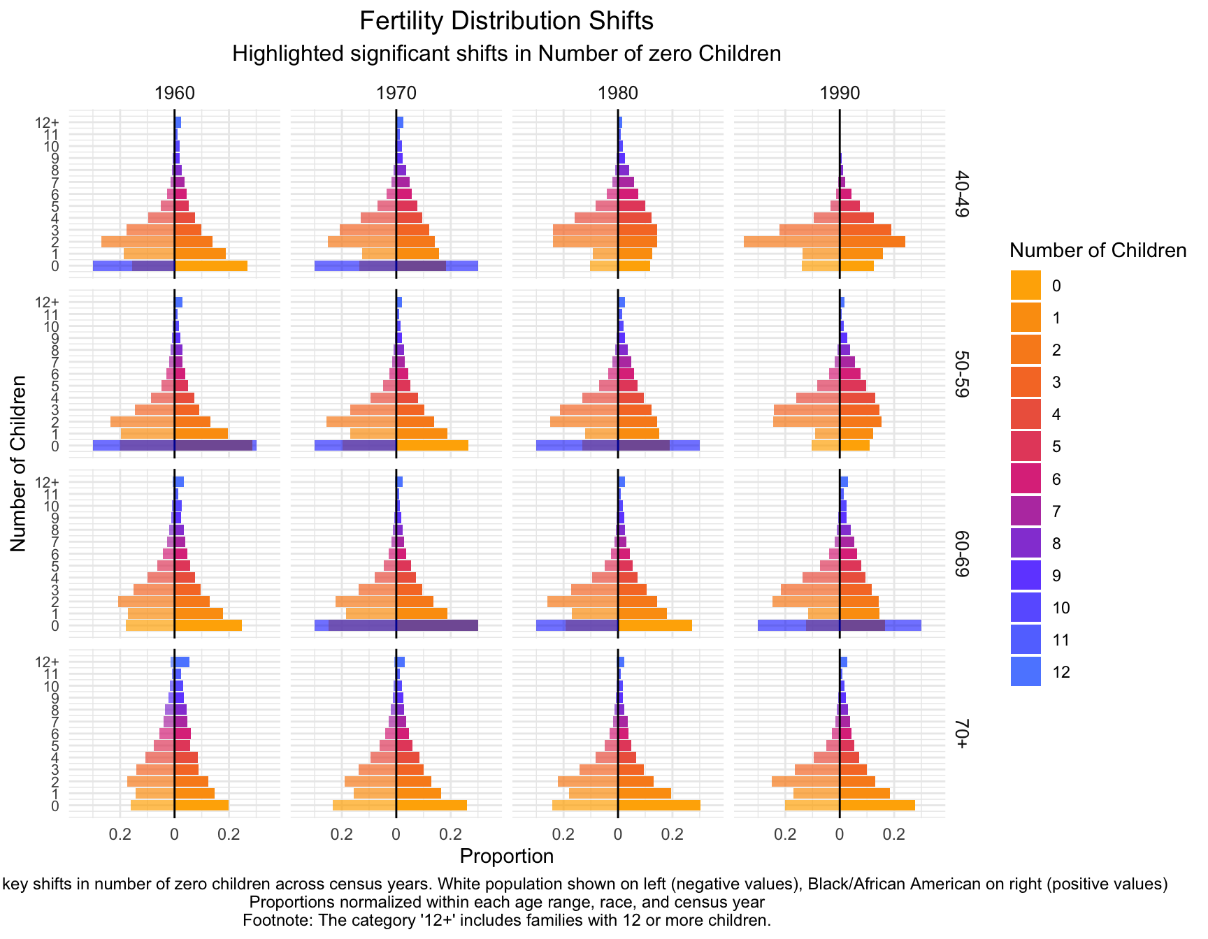
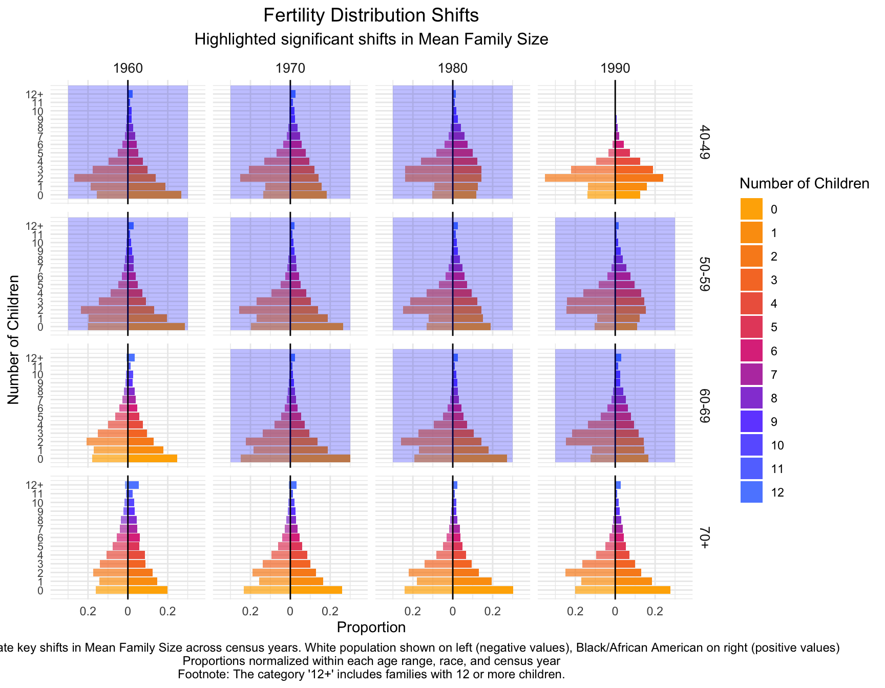
child_plot +
  geom_rect(data = df_mirror %>% filter((YEAR == 1960 & AGE_RANGE == "40-49")|
                                        (YEAR == 1960 & AGE_RANGE == "50-59")|
                                        (YEAR == 1970 & AGE_RANGE == "40-49")|
                                        (YEAR == 1970 & AGE_RANGE == "50-59")|
                                        (YEAR == 1970 & AGE_RANGE == "60-69")|
                                        (YEAR == 1980 & AGE_RANGE == "40-49")|
                                        (YEAR == 1980 & AGE_RANGE == "50-59")|
                                        (YEAR == 1980 & AGE_RANGE == "60-69")|
                                        (YEAR == 1990 & AGE_RANGE == "50-59")|
                                        (YEAR == 1990 & AGE_RANGE == "60-69")),
            aes(xmin = -0.45, xmax = 13, ymin = -0.3, ymax = 0.3),
            fill = "blue", alpha = 0.01) +
  labs(title = "Fertility Distribution Shifts",
       subtitle = "Highlighted significant shifts in Mean Family Size",
       caption = "Annotations indicate key shifts in Mean Family Size across census years. White population shown on left (negative values), Black/African American on right (positive values)\nProportions normalized within each age range, race, and census year\nFootnote: The category '12+' includes families with 12 or more children.") +
  theme_minimal()+
  theme(
    plot.title = element_text(size = 14, hjust = 0.5),
    plot.subtitle = element_text(size = 12, hjust = 0.5),
    plot.caption = element_text(size = 9, hjust = 0.5),
    axis.text.y = element_text(size = 8),
    strip.text = element_text(size = 10)
  )
2.2 Panel B: Comparison of 40-49 and 50-59 Age Groups in 1990
- Create Comparative Distribution Plots:
- Generate side-by-side or overlaid histograms or density plots for the 40-49 and 50-59 age groups within each racial group.
- Include Summary Statistics:
- On each plot or in accompanying tables, provide:
- Mean number of children
- Variance
- Proportion of women with zero children (zero inflation)
- On each plot or in accompanying tables, provide:
- Ensure Clarity in Visuals:
- Properly label axes, legends, and titles.
- Use consistent color schemes for easy comparison between groups.
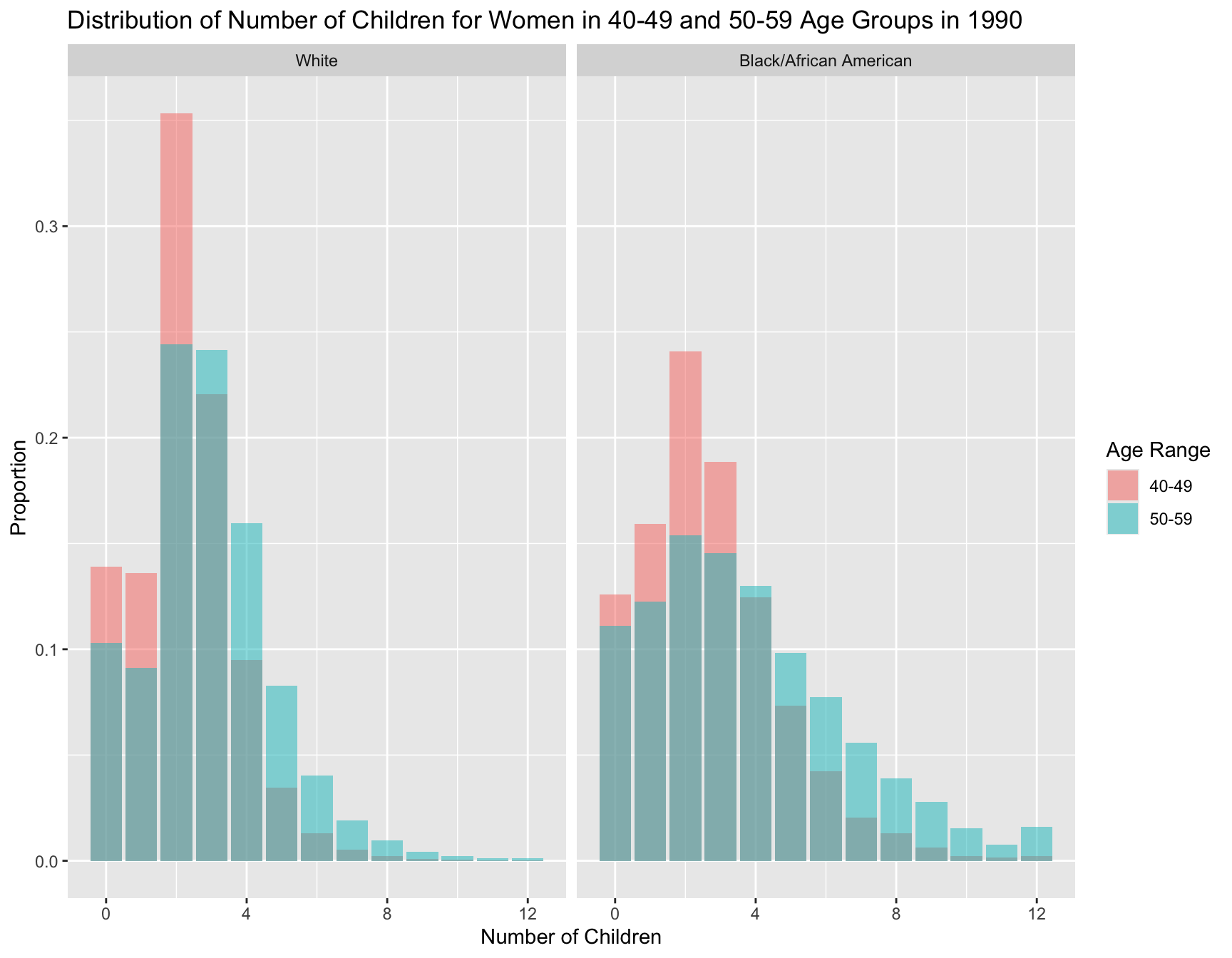
filter_df <- df_proportions %>%
  filter(YEAR == "1990", AGE_RANGE %in% c("40-49", "50-59"))
ggplot(filter_df, aes(x = chborn_num, y = proportion, fill = AGE_RANGE)) +
geom_col(position = "identity", alpha = 0.5) +
facet_wrap(~ RACE) +
labs(
title = "Distribution of Number of Children for Women in 40-49 and 50-59 Age Groups in 1990",
x = "Number of Children",
y = "Proportion",
fill = "Age Range"
) 
| Version | Author | Date |
|---|---|---|
| 776920f | linmatch | 2024-11-12 |
summary_stats <- filter_df %>%
  group_by(AGE_RANGE, RACE) %>%
  summarise(
    mean_children = weighted.mean(chborn_num, count),  # Mean number of children
    variance_children = sum(count * (chborn_num - weighted.mean(chborn_num, count))^2) / sum(count),  # Variance
    zero_inflation = sum(count[chborn_num == 0]) / sum(count)  # Proportion of women with 0 children
  )
`summarise()` has grouped output by 'AGE_RANGE'. You can override using the
`.groups` argument.# Print summary statistics table
summary_stats# A tibble: 4 × 5
# Groups: AGE_RANGE [2]
AGE_RANGE RACE mean_children variance_children zero_inflation
<chr> <fct> <dbl> <dbl> <dbl>
1 40-49 White 2.20 2.09 0.139
2 40-49 Black/African Americ… 2.69 3.96 0.126
3 50-59 White 2.89 3.35 0.103
4 50-59 Black/African Americ… 3.72 7.74 0.111Step 3: Perform Statistical Comparisons
Conduct statistical tests to determine if observed differences are significant.
3.1 T-Test for Difference in Means
- Compare Means Between Age Groups:
- For each racial group, perform a t-test to compare the mean number of children between the 40-49 and 50-59 age groups.
- Check Assumptions:
- Ensure that the data meets the assumptions of the t-test (normality, equal variances).
- If assumptions are violated, consider using a non-parametric test like the Mann-Whitney U test.
## Check the normality assumption for black population
# Subset data for the 40-49 and 50-59 age groups
data_40_49_b <- df %>% filter(AGE_RANGE == "40-49", RACE == "Black/African American")
data_50_59_b <- df %>% filter(AGE_RANGE == "50-59", RACE == "Black/African American")

qqnorm(data_40_49_b$chborn_num, main = "QQ Plot: 40-49 Age Group (Black/African American)")
qqline(data_40_49_b$chborn_num)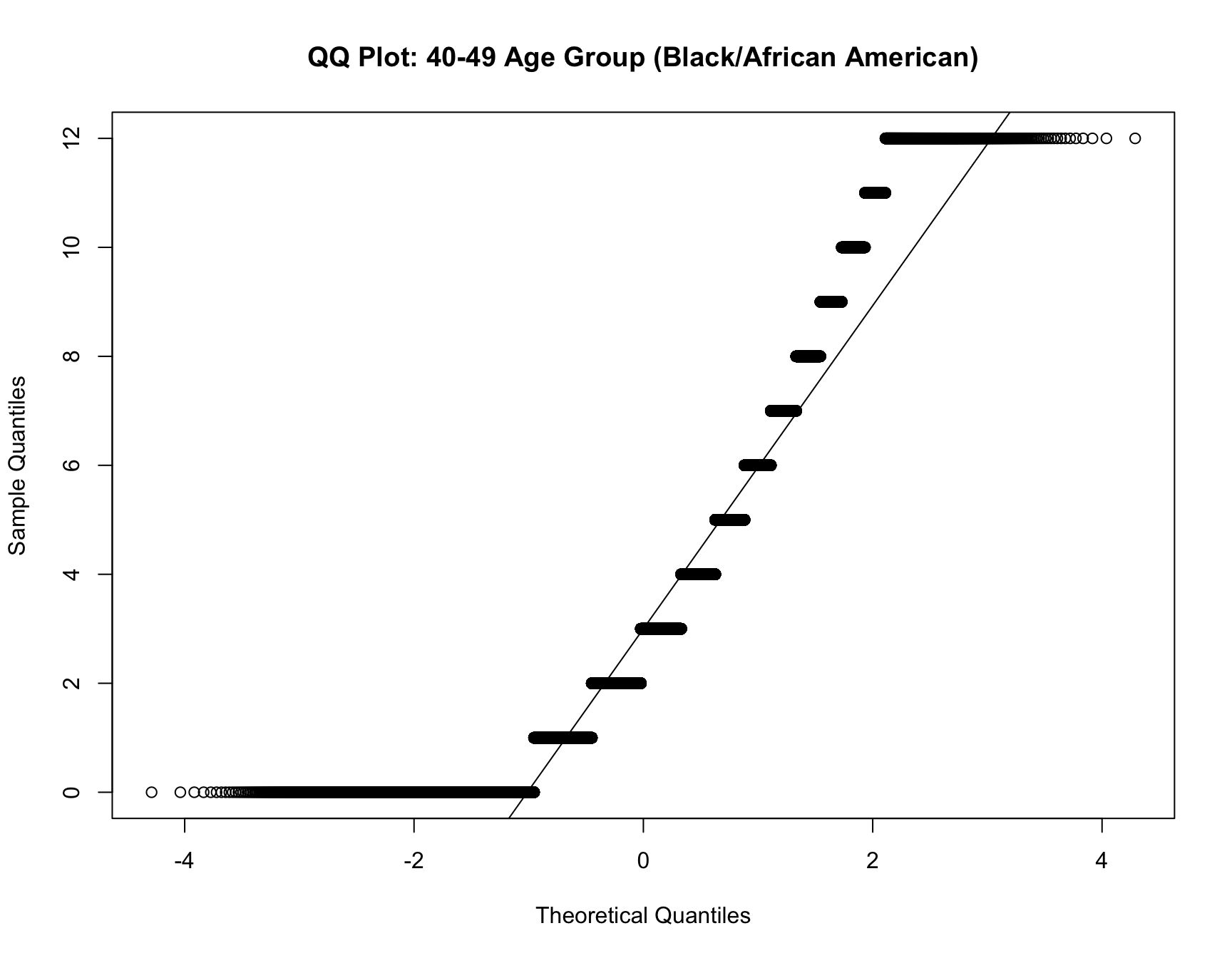
| Version | Author | Date |
|---|---|---|
| 776920f | linmatch | 2024-11-12 |
# QQ plot for the 50-59 age group
qqnorm(data_50_59_b$chborn_num, main = "QQ Plot: 50-59 Age Group (Black/African American)")
qqline(data_50_59_b$chborn_num)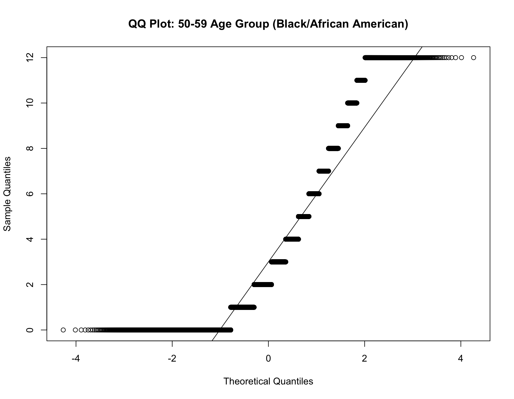
## Check equal variance for black population
df_b <- df %>% filter(RACE == "Black/African American")

# Levene's test for equal variances
levene_test_result <- leveneTest(chborn_num ~ as.factor(AGE_RANGE), data = df_b)

levene_test_result
Levene's Test for Homogeneity of Variance (center = median)
Df F value Pr(>F)
group 3 93.887 < 2.2e-16 ***
176718
---
Signif. codes: 0 '***' 0.001 '**' 0.01 '*' 0.05 '.' 0.1 ' ' 1## Check the normality assumption for white population
data_40_49_w <- df %>% filter(AGE_RANGE == "40-49", RACE == "White")
data_50_59_w <- df %>% filter(AGE_RANGE == "50-59", RACE == "White")
qqnorm(data_40_49_w$chborn_num, main = "QQ Plot: 40-49 Age Group (White)")
qqline(data_40_49_w$chborn_num)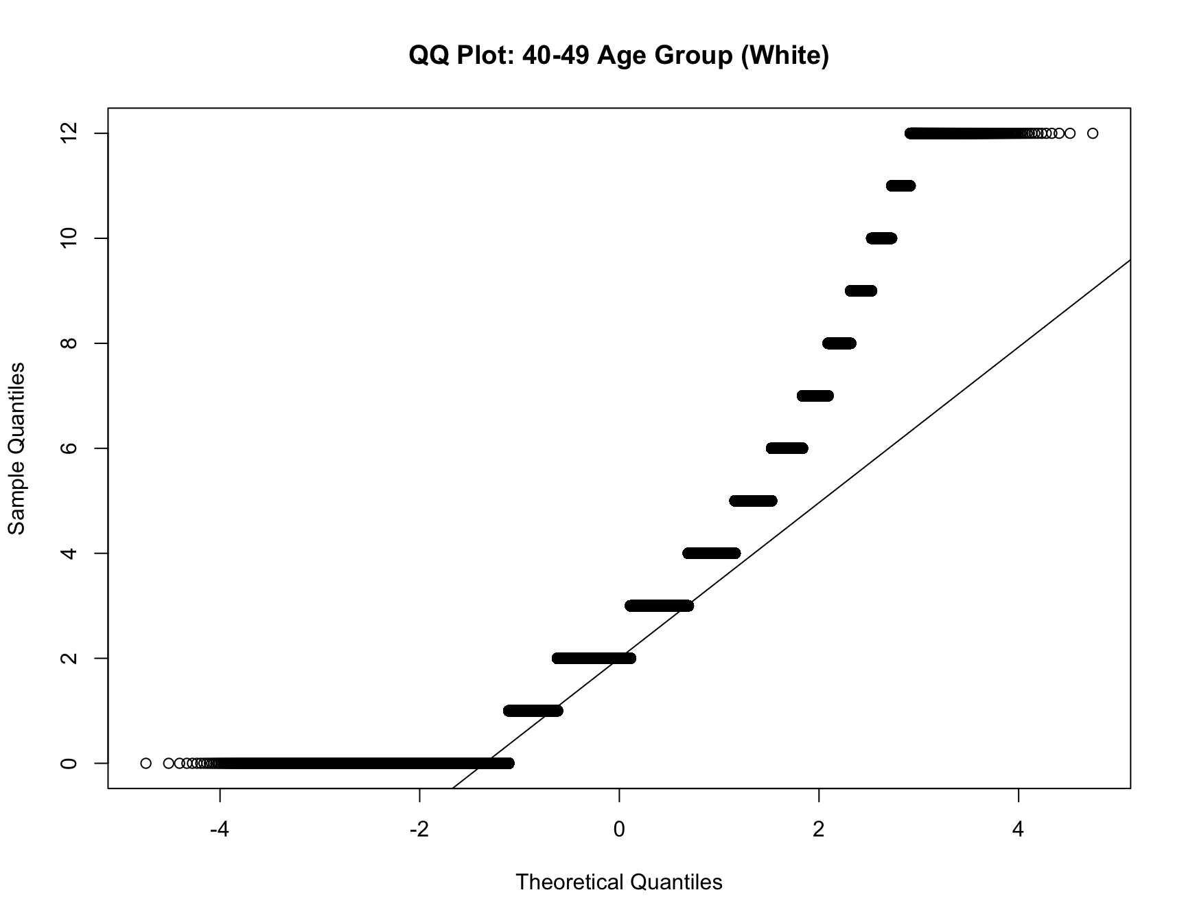
# QQ plot for the 50-59 age group
qqnorm(data_50_59_w$chborn_num, main = "QQ Plot: 50-59 Age Group (White)")
qqline(data_50_59_w$chborn_num)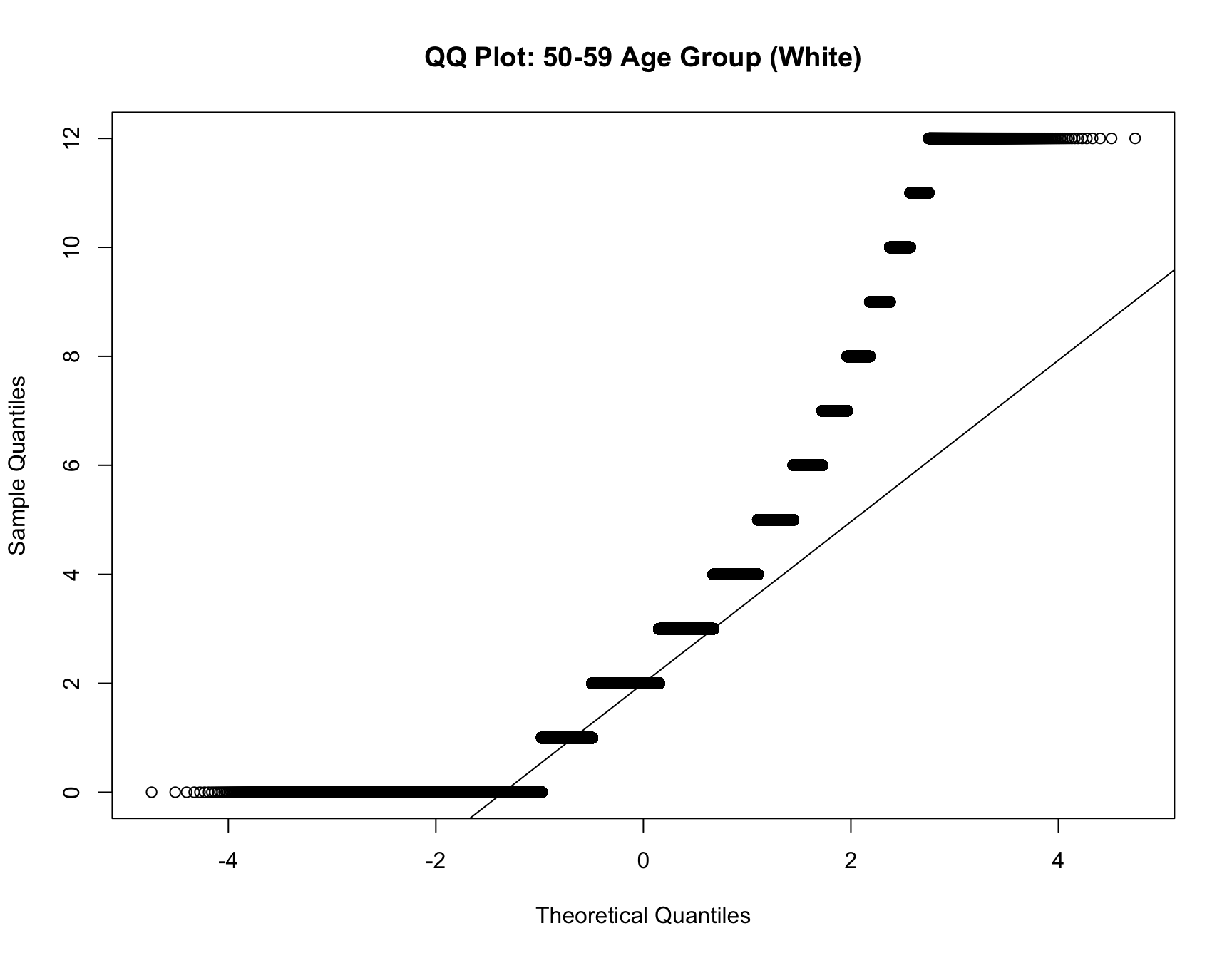
## Check equal variance for white population
df_w <- df %>% filter(RACE == "White")

# Levene's test for equal variances
levene_test_result2 <- leveneTest(chborn_num ~ as.factor(AGE_RANGE), data = df_w)

levene_test_result2
Levene's Test for Homogeneity of Variance (center = median)
Df F value Pr(>F)
group 3 4205.8 < 2.2e-16 ***
1740751
---
Signif. codes: 0 '***' 0.001 '**' 0.01 '*' 0.05 '.' 0.1 ' ' 1Since the data for black population and white population violate both assumption, we perform a Mann-Whitney U test for both racial groups in the follwoing:
wilcox_test_result <- wilcox.test(data_40_49_b$chborn_num, data_50_59_b$chborn_num)$p.value
wilcox_test_result2 <- wilcox.test(data_40_49_w$chborn_num, data_50_59_w$chborn_num)$p.value
print(c(wilcox_test_result, wilcox_test_result2))
[1] 1.012022e-31 3.463246e-126RESULT: These p-values are both extremely small (close to zero), meaning there is a very strong statistical difference between the two age groups (40-49 and 50-59) in terms of the number of children within each racial group.
3.2 F-Test for Difference in Variances
- Assess Variance Differences:
- Perform an F-test or Levene’s test to compare the variances of the number of children between the two age groups within each racial group.
## Apply Levene's test since non-normality

# Levene's test for Black group
levene_test_b <- leveneTest(chborn_num ~ as.factor(AGE_RANGE), data = df_b)

# Levene's test for White group
levene_test_w <- leveneTest(chborn_num ~ as.factor(AGE_RANGE), data = df_w)

# Print results
print(levene_test_b)
Levene's Test for Homogeneity of Variance (center = median)
Df F value Pr(>F)
group 3 93.887 < 2.2e-16 ***
176718
---
Signif. codes: 0 '***' 0.001 '**' 0.01 '*' 0.05 '.' 0.1 ' ' 1print(levene_test_w)Levene's Test for Homogeneity of Variance (center = median)
Df F value Pr(>F)
group 3 4205.8 < 2.2e-16 ***
1740751
---
Signif. codes: 0 '***' 0.001 '**' 0.01 '*' 0.05 '.' 0.1 ' ' 1RESULT: Since the p values are smaller than 0.05 for both racial group, we have enough evidence to reject the null hypothesis, indicating that the variances of the number of children between the two age groups within each racial group are significantly different.
3.3 Chi-Square Test for Difference in Zero Inflation
- Analyze Zero Inflation:
- Create contingency tables showing the counts of women with zero children and those with one or more children for each age group.
- Perform a chi-square test to determine if the proportion of childlessness differs significantly between the age groups within each racial group.
ZI_table <- df %>%
  mutate(childlessness = ifelse(chborn_num == 0, "0 Children", "1+ Children")) %>%       group_by(RACE, AGE_RANGE, childlessness) %>%
  summarise(count = n())
`summarise()` has grouped output by 'RACE', 'AGE_RANGE'. You can override using
the `.groups` argument.ZI_table# A tibble: 16 × 4
# Groups: RACE, AGE_RANGE [8]
RACE AGE_RANGE childlessness count
<fct> <chr> <chr> <int>
1 White 40-49 0 Children 63463
2 White 40-49 1+ Children 410055
3 White 50-59 0 Children 76528
4 White 50-59 1+ Children 391044
5 White 60-69 0 Children 77238
6 White 60-69 1+ Children 320508
7 White 70+ 0 Children 87293
8 White 70+ 1+ Children 314626
9 Black/African American 40-49 0 Children 9469
10 Black/African American 40-49 1+ Children 46173
11 Black/African American 50-59 0 Children 10846
12 Black/African American 50-59 1+ Children 39202
13 Black/African American 60-69 0 Children 9907
14 Black/African American 60-69 1+ Children 29176
15 Black/African American 70+ 0 Children 8575
16 Black/African American 70+ 1+ Children 23374ZI_table_b <- ZI_table %>%
filter(RACE == "Black/African American")
cont_table_b <- xtabs(count ~ AGE_RANGE + childlessness, data = ZI_table_b)
chi_test_b <- chisq.test(cont_table_b)
chi_test_b
    Pearson's Chi-squared test

data:  cont_table_b
X-squared = 1501.6, df = 3, p-value < 2.2e-16
ZI_table_w <- ZI_table %>%
filter(RACE == "White")
cont_table_w <- xtabs(count ~ AGE_RANGE + childlessness, data = ZI_table_w)
chi_test_w <- chisq.test(cont_table_w)
chi_test_w
    Pearson's Chi-squared test

data:  cont_table_w
X-squared = 11896, df = 3, p-value < 2.2e-16
RESULT: The p-values for both tests are extremely low, suggests that there is a significant difference in the proportion of women with 0 children across different age ranges for both the Black/African American and White racial groups. The results imply that childlessness is not uniformly distributed across age groups.
Step 4: Summarize Findings
Write a clear and concise summary addressing the following points.
4.1 Significant Fertility Shifts Across Cohorts
- Identify Timing of Shifts:
- Specify when significant fertility shifts occurred for each racial group based on your analysis in Question 2.
- Describe Nature of Shifts:
- Detail the characteristics of the shifts, such as:
- Decrease in mean number of children
- Increase in childlessness (zero inflation)
- Changes in variance or distribution shape
- Detail the characteristics of the shifts, such as:
- Highlight Differences Between Racial Groups:
- Compare the timing and nature of shifts between African American and European American women.
- Discuss any patterns or discrepancies observed.
4.2 Comparison of 40-49 and 50-59 Age Groups in 1990
- Summarize Key Differences:
- Present the differences in fertility patterns between the two age groups for each racial group.
- Include comparisons of:
- Distribution shapes
- Mean number of children
- Variance
- Zero inflation
- Report Statistical Test Results:
- Provide the results of the t-tests, F-tests, and chi-square tests.
- Interpret the significance of these results in the context of your analysis.
- Discuss Implications:
- Consider what these differences suggest about fertility trends and behaviors.
- Reflect on whether the older age group represents completed fertility patterns.
4.3 Synthesis and Implications
- Integrate Findings:
- Connect the insights from the cohort analysis with the age group comparison.
- Discuss how the patterns observed in the 1990 census relate to the shifts identified across cohorts.
- Consider Contributing Factors:
- Explore potential social, economic, or policy factors that may have
contributed to the observed fertility shifts.
- For example, changes in access to education, employment opportunities, or family planning resources.
- Explore potential social, economic, or policy factors that may have
contributed to the observed fertility shifts.
- Reflect on Broader Implications:
- Discuss how these fertility trends might impact your broader research topic, such as genetic surveillance disparities.
- Consider the implications for future demographic research or policy development.
Additional Considerations
- Visual Clarity:
- Ensure all visualizations are easy to interpret.
- Use clear labels, legends, and annotations.
- Contextualize Statistical Significance:
- Explain not just whether results are statistically significant, but also what they mean in practical terms.
- Acknowledge Data Limitations:
- Discuss any limitations or biases in the data that could affect your
findings.
- For instance, sample size constraints or missing data.
- Discuss any limitations or biases in the data that could affect your
findings.
- Ethical Considerations:
- Approach discussions of race and fertility sensitively and responsibly.
- Avoid drawing causal conclusions without robust evidence.
Integration with Previous Work
- Leverage Previous Analyses:
- Use the visualizations and statistical summaries from Questions 1 and 2 as foundations for this analysis.
- Create a Cohesive Narrative:
- Ensure that your findings from all questions are connected and build upon each other.
- Tell a comprehensive story about fertility trends across cohorts and racial groups.
Final Deliverables
- Multi-Panel Visualization:
- Panel A: Fertility distribution shifts across cohorts with highlighted significant shifts.
- Panel B: Comparative distribution plots for 40-49 and 50-59 age groups in 1990, including summary statistics.
- Written Summary:
- A concise report that addresses the points outlined in Step 4.
- Include interpretations of statistical analyses and discuss broader implications.
- Statistical Analysis Documentation:
- Provide details of the statistical tests conducted, including test assumptions, results, and interpretations.
- Annotated Code (if applicable):
- While not the focus, include any new code used for this analysis with appropriate comments.
Distribution of Number of Siblings Across Census Years
Having analyzed the distribution of the number of children, we now turn our attention to the distribution of the number of siblings. We will explore the trends in the frequency of the number of siblings for African American and European American mothers across the Census years by age group.
Frequency of siblings is calculated as follows.
\[ \text{freq}_{n_{\text{sib}}} = \text{freq}_{\text{mother}} \cdot \text{chborn}_{\text{num}} \]
For example, suppose 10 mothers (generation 0) have 7 children, then there will be 70 children (generation 1) in total who each have 6 siblings.
We take our original data and calculate the frequency of siblings for each mother based on the number of children they have. We then aggregate this data to get the frequency of siblings for each generation along with details on the birthyears of the relevant children to visualize the distribution of the number of siblings across generations.
[Instructions for Manqing] Plot Across Census Years for Children
Objective
Create a mirror plot for the distribution of siblings across census years, races, and birth ranges, similar to the one created for the number of children.
Step 1: Calculate Sibling Frequencies
- Start with your dataframe that includes the
AGE_RANGEcolumn.
df2 <- df %>%
dplyr::select(RACE, YEAR, AGE_RANGE, chborn_num)- Create a new column for the number of siblings:
df2 <- df2 %>%
mutate(n_siblings = chborn_num - 1)- Calculate the frequency of siblings:
df2 <- df2 %>%
mutate(sibling_freq = ifelse(chborn_num != 1, n_siblings * 1, 1))  # Assuming each mother represents 1 in frequency
Step 2: Aggregate Sibling Data
- Group the data and calculate sibling frequencies:
df_siblings <- df2 %>%
 group_by(YEAR, RACE, AGE_RANGE, n_siblings) %>%
 summarise(
   sibling_count = sum(sibling_freq),
   .groups = "drop"
)- Calculate proportions within each group:
df_sibling_proportions <- df_siblings %>%
 group_by(YEAR, RACE, AGE_RANGE) %>%
 mutate(proportion = sibling_count / sum(sibling_count)) %>%
 ungroup()
Step 3: Check Normalization
Before creating the plot, verify that the proportions are correctly normalized:
normalization_check <- df_sibling_proportions %>%
  group_by(YEAR, RACE, AGE_RANGE) %>%
  summarise(total_proportion = sum(proportion), .groups = "drop") %>%
  arrange(YEAR, RACE, AGE_RANGE)

print(normalization_check)
# A tibble: 32 × 4
YEAR RACE AGE_RANGE total_proportion
<int> <fct> <chr> <dbl>
1 1960 White 40-49 1
2 1960 White 50-59 1
3 1960 White 60-69 1
4 1960 White 70+ 1
5 1960 Black/African American 40-49 1
6 1960 Black/African American 50-59 1
7 1960 Black/African American 60-69 1
8 1960 Black/African American 70+ 1
9 1970 White 40-49 1
10 1970 White 50-59 1
# ℹ 22 more rowsEnsure that the total_proportion for each group is very
close to 1.0. If not, revisit your calculations in Step 2.
Step 4: Prepare Data for Mirror Plot
Reshape data for the mirror plot:
df_sibling_mirror <- df_sibling_proportions %>%
  mutate(proportion = if_else(RACE == "White", -proportion, proportion))
Step 5: Create the Mirror Plot
- Create the color palette:
my_colors <- colorRampPalette(c("#FFB000", "#F77A2E", "#DE3A8A", "#7253FF", "#5E8BFF"))(13)- Create the plot:
ggplot(data = df_sibling_mirror %>% filter(n_siblings != "-1"), aes(x = n_siblings, y = proportion, fill = as.factor(n_siblings))) +
 geom_col(aes(alpha = RACE)) +
 geom_hline(yintercept = 0, color = "black", size = 0.5) +
 facet_grid(AGE_RANGE ~ YEAR, scales = "free_y") +
 coord_flip() +
 scale_y_continuous(
   labels = function(x) abs(x),
   limits = function(x) c(-max(abs(x)), max(abs(x)))
 ) +
 scale_x_continuous(breaks = 0:11, labels = c(0:10, "11+")) +
 scale_fill_manual(values = my_colors) +
 scale_alpha_manual(values = c("White" = 0.7, "Black/African American" = 1)) +
 labs(
   title = "Distribution of Number of Siblings by Census Year, Race, and Age Range",
   x = "Number of Siblings",
   y = "Proportion",
   fill = "Number of Siblings",
   caption = "White population shown on left (negative values), Black/African American on right (positive values)\nProportions normalized within each age range, race, and census year\nFootnote: The category '11+' includes individuals with 11 or more siblings."
 ) +
 theme_minimal() +
 theme(
   plot.title = element_text(size = 14, hjust = 0.5),
   axis.text.y = element_text(size = 8),
   strip.text = element_text(size = 10),
   legend.position = "none",
   panel.grid.major.y = element_blank(),
   panel.grid.minor.y = element_blank()
 )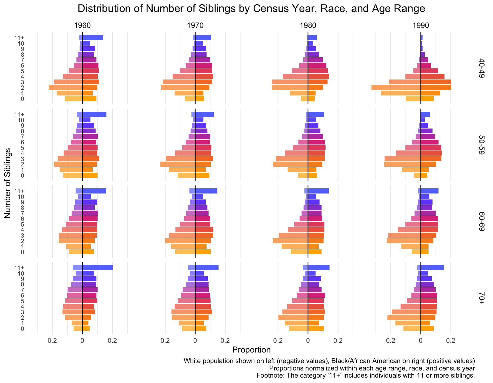
Step 6: Interpret the Plot
After creating the plot, examine it carefully:
- Look for patterns in sibling distribution across different census years and age ranges.
RESULT:
-By Census Year: In 1960 and 1970, individuals are more likely to have higher number of siblings, especially in the 5-10 range. This trend diminishes over time.
By 1980 and 1990, the distribution shifts toward smaller family sizes, with a growing proportion of individuals having fewer siblings.
-By age range:
40-49 Age Group: For this group, the number of individuals with 0-2 siblings increases across census years, especially in 1980 and 1990, while the proportion of individuals with larger sibling counts decreases.
50-59 and 60-69 Age Groups: These groups show a similar shift toward smaller family sizes, but the trend is slightly more gradual compared to the younger age group.
70+ Age Group: The shift to fewer siblings is noticeable, although the trend is less pronounced. The distribution remains relatively stable across the census years, with a significant portion of individuals still coming from large families in 1960 and 1970.
- Compare the distributions between White and Black/African American populations.
RESULT: -Black/African American Populations (right side of each pair) consistently show a higher proportion of individuals with larger sibling counts (5-10 siblings) compared to White populations. However, similar to the White population, the number of individuals with fewer siblings increases over time.
- Note any significant changes or trends in the number of siblings over time.
RESULT: -White Populations: (left side of each pair) have a more marked shift toward smaller families by 1990, with a larger proportion of individuals having 0-2 siblings compared to the Black/African American population. The decline in larger family sizes (5+ siblings) is more pronounced among Whites, particularly by 1980 and 1990.
- Consider how these sibling distributions might differ from the children distributions you analyzed earlier, and think about potential reasons for these differences.
RESULT: While both distributions show a trend toward smaller families, the sibling distribution is more spread out across different sibling counts, suggesting potential difference in the distribution.
[Instructions for Manqing] Model Fit Across Census Years
Objective
Repeat the model fitting process we performed for the children distribution, this time using the sibling distribution data.
Steps
Prepare the Sibling Data Use the sibling distribution data you calculated earlier (
df_sibling_proportions).Fit Models For each combination of RACE, YEAR, and AGE_RANGE, fit the following distributions:
- Poisson
- Negative Binomial
- Zero-Inflated Poisson
- Zero-Inflated Negative Binomial
Use the same R functions and packages as in the children distribution analysis.
Compare Model Fits Use AIC (Akaike Information Criterion) to compare the fits of different models for each group.
combinations2 <- df2 %>%
  # treat number of sib = -1 as NA
  filter(n_siblings != -1) %>%
  group_by(YEAR, RACE, AGE_RANGE) %>%
  group_split()

# Initialize the data frame to store results
best_models_sib <- data.frame(
  Race = character(),
  Census_Year = numeric(),
  AGE_RANGE = character(),
  AIC_poisson = numeric(),
  AIC_nb = numeric(),
  AIC_zip = numeric(),
  AIC_zinb = numeric(),
  stringsAsFactors = FALSE
)

# Loop through each subset of data
for (i in seq_along(combinations2)) {
  subset_data <- combinations2[[i]]

  # Fit Poisson model
  poisson_model <- glm(n_siblings ~ 1, family = poisson, data = subset_data)
  # Fit Negative Binomial model
  nb_model <- glm.nb(n_siblings ~ 1, data = subset_data)

  # Fit Zero-Inflated Poisson model
  zip_model <- zeroinfl(n_siblings ~ 1 | 1, data = subset_data, dist = "poisson",control = zeroinfl.control(maxit = 100))

  # Fit Zero-Inflated Negative Binomial model with increased max iterations
  zinb_model <- zeroinfl(n_siblings ~ 1 | 1, data = subset_data, dist = "negbin",control = zeroinfl.control(maxit = 100))

  # Append the result to the best_models data frame
  best_models_sib <- rbind(
    best_models_sib,
    data.frame(
      Race = unique(subset_data$RACE),
      Census_Year = unique(subset_data$YEAR),
      AGE_RANGE = unique(subset_data$AGE_RANGE),
      AIC_poisson = AIC(poisson_model),
      AIC_nb = AIC(nb_model),
      AIC_zip = AIC(zip_model),
      AIC_zinb = AIC(zinb_model),
      stringsAsFactors = FALSE
    )
  )
}- Identify Best-Fitting Models Determine which model fits best for each combination of RACE, YEAR, and AGE_RANGE.
# Add a Best_Model column to store the best model based on minimum AIC
best_models_sib$Best_Model <- apply(best_models_sib, 1, function(row) {
  # Get AIC values for Poisson, NB, ZIP, and ZINB models
  aic_values <- c(Poisson = as.numeric(row['AIC_poisson']),
                  Negative_Binomial = as.numeric(row['AIC_nb']),
                  Zero_Inflated_Poisson = as.numeric(row['AIC_zip']),
                  Zero_Inflated_NB= as.numeric(row['AIC_zinb']))

  # Find the name of the model with the minimum AIC value
  best_models_sib <- names(which.min(aic_values))

  return(best_models_sib)
})

best_models_sib <- best_models_sib %>% dplyr::select(Race, Census_Year, AGE_RANGE, Best_Model)
# View the updated table with the Best_Model column
print(best_models_sib)
Race Census_Year AGE_RANGE Best_Model
1 White 1960 40-49 Negative_Binomial
2 White 1960 50-59 Negative_Binomial
3 White 1960 60-69 Negative_Binomial
4 White 1960 70+ Negative_Binomial
5 Black/African American 1960 40-49 Zero_Inflated_NB
6 Black/African American 1960 50-59 Zero_Inflated_NB
7 Black/African American 1960 60-69 Zero_Inflated_NB
8 Black/African American 1960 70+ Zero_Inflated_NB
9 White 1970 40-49 Negative_Binomial
10 White 1970 50-59 Negative_Binomial
11 White 1970 60-69 Negative_Binomial
12 White 1970 70+ Negative_Binomial
13 Black/African American 1970 40-49 Zero_Inflated_NB
14 Black/African American 1970 50-59 Zero_Inflated_NB
15 Black/African American 1970 60-69 Zero_Inflated_NB
16 Black/African American 1970 70+ Zero_Inflated_NB
17 White 1980 40-49 Negative_Binomial
18 White 1980 50-59 Negative_Binomial
19 White 1980 60-69 Negative_Binomial
20 White 1980 70+ Negative_Binomial
21 Black/African American 1980 40-49 Zero_Inflated_NB
22 Black/African American 1980 50-59 Zero_Inflated_NB
23 Black/African American 1980 60-69 Zero_Inflated_NB
24 Black/African American 1980 70+ Zero_Inflated_NB
25 White 1990 40-49 Poisson
26 White 1990 50-59 Negative_Binomial
27 White 1990 60-69 Negative_Binomial
28 White 1990 70+ Negative_Binomial
29 Black/African American 1990 40-49 Negative_Binomial
30 Black/African American 1990 50-59 Zero_Inflated_NB
31 Black/African American 1990 60-69 Zero_Inflated_NB
32 Black/African American 1990 70+ Zero_Inflated_NB- Analyze Patterns
- Examine how the best-fitting model changes across years and birth ranges for each race.
- Compare these patterns to those observed in the children distribution analysis.
- Visualize Results Create a summary plot showing the best-fitting models across years and birth ranges for each race, similar to the one created for the children distribution.
# Bar plot showing the distribution of best models across races
ggplot(best_models_sib, aes(x = Race, fill = Best_Model)) +
  geom_bar(position = "stack") +
  labs(title = "Best-Fitting Models (siblings) by Race", x = "Race", y = "Count", fill = "Best Model")
# Bar plot showing the distribution of best models across races
ggplot(best_models_sib, aes(x = Census_Year, fill = Best_Model)) +
geom_bar(position = "stack") +
labs(title = "Best-Fitting Models (siblings) by Census Year", x = "Census Year", y = "Count", fill = "Best Model")# Bar plot showing the distribution of best models across races
ggplot(best_models_sib, aes(x = AGE_RANGE, fill = Best_Model)) +
geom_bar(position = "stack") +
labs(title = "Best-Fitting Models (siblings) by Birth Range)", x = "Age Range", y = "Count", fill = "Best Model")ggplot(best_models_sib, aes(x = Census_Year, y = AGE_RANGE, fill = Best_Model)) +
geom_tile(color = "white", lwd = 0.5, linetype = 1) + # Create the tiles
facet_wrap(~Race, nrow = 2) + # Facet by Race
scale_fill_manual(values = c("Poisson" = "#0072B2", "Zero_Inflated_NB" = "#F0E442", "Negative_Binomial" = "grey")) +
labs(
title = "Best Model(siblings) by Race, Census Year, and Birth Range",
x = "Census Year",
y = "Age Range",
fill = "Best Model"
) +
theme_minimal() +
theme(
axis.text.x = element_text(angle = 45, hjust = 1), # Rotate x-axis labels for readability
plot.title = element_text(size = 14, face = "bold"),
legend.position = "bottom"
)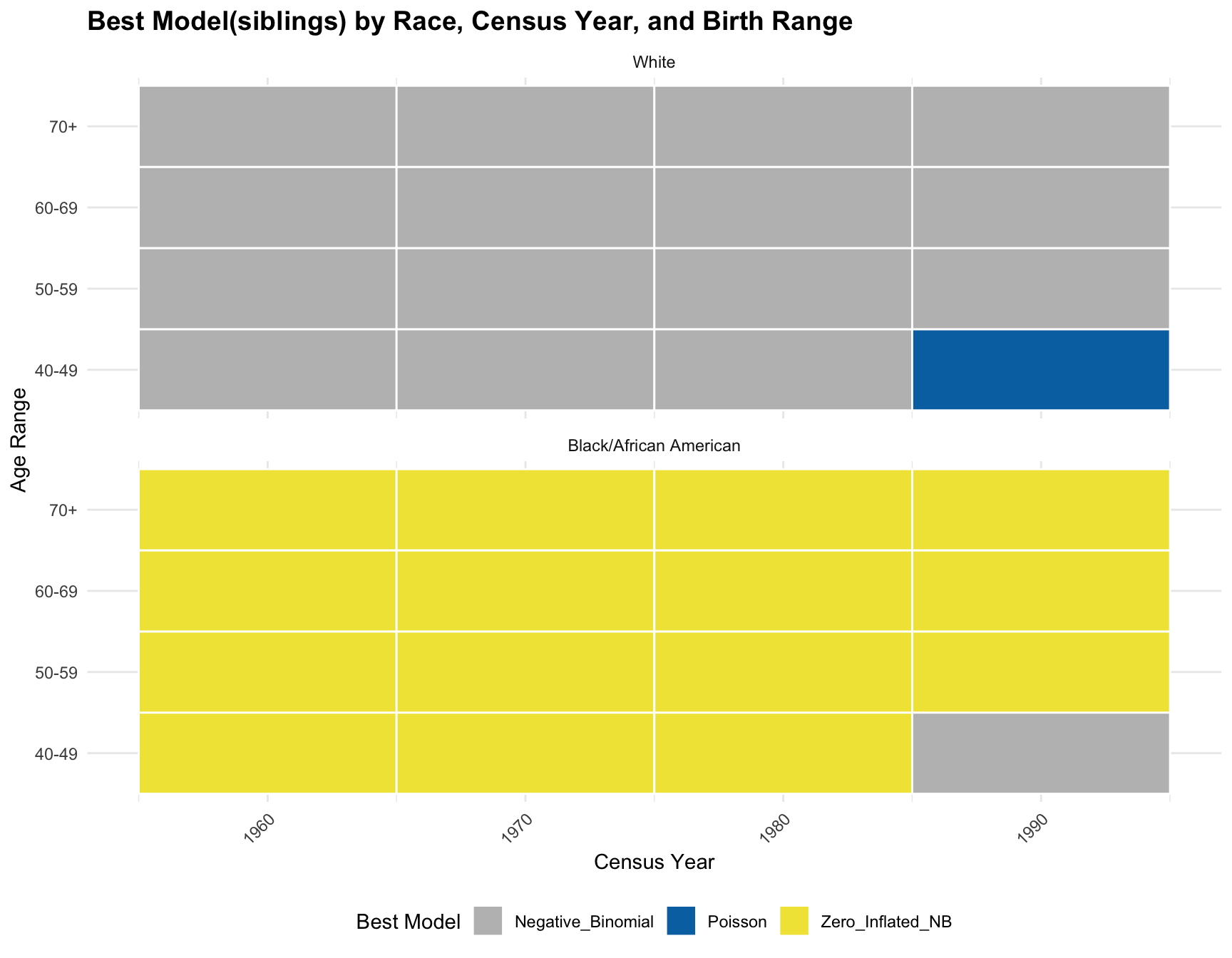
- Interpret Findings
- Discuss any differences in the best-fitting models between the sibling and children distributions.
RESULT: By comparing the pattern of best-fitting models between the sibling and children distributions, we observe that the best model for black population has the same best model(zero-inlfated NB) across year and age range except on one subset(age 40-49 in 1990) in siblings distribution. However, there is a large difference in best model for white population. A large portion of best model in children distribution for white population is zero-inlfated NB, while negative-binomial is the best model fitted for siblings distribution except for one subset(age 40-49 in 1990).
- Consider the implications of these differences for understanding family structures and fertility patterns.
[Instructions for Manqing] Cohort Stability Analysis Siblings
Objective
Analyze the stability of sibling distributions across cohorts, similar to the analysis performed for children.
Steps
Use the sibling distribution data (
df_sibling_proportions).For each combination of RACE and birth_range:
- Compare the sibling distributions across different census years.
- Use statistical tests (e.g., Kolmogorov-Smirnov test) to assess if distributions are significantly different.
 df_sibling_proportions <- df_sibling_proportions %>%
  mutate(Cohort = mapply(calculate_cohort, YEAR, AGE_RANGE))
df_sibling_proportions %>%
filter(n_siblings >= 0, sibling_count >= 0, proportion >= 0) %>% group_by(RACE, Cohort) %>%
ggplot(aes(x = n_siblings, y = proportion, color = as.factor(YEAR))) +
geom_line() +
labs(
title = "Sibling Distribution by Census Year",
x = "Number of Siblings",
y = "Proportion",
color = "Census Year"
) +
facet_grid(RACE ~ Cohort) +
theme_minimal()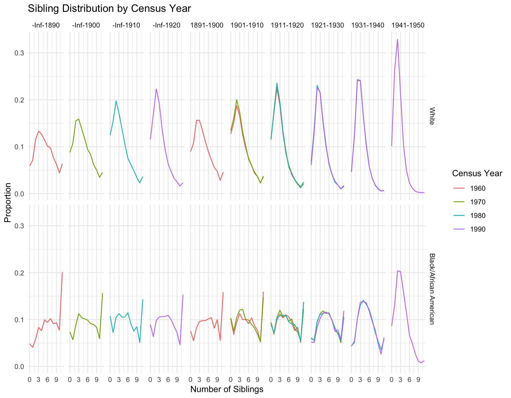
df_sibling_b <- df_sibling_proportions %>% filter(RACE == "Black/African American", n_siblings >= 0, sibling_count >= 0, proportion >= 0)

results_sib_b <- list()

cohort_counts2 <- df_sibling_b %>%
  group_by(Cohort) %>%
  summarise(Unique_Census_Years = n_distinct(YEAR)) %>%
  filter(Unique_Census_Years > 1)

for (cohort in cohort_counts2$Cohort) {
  cohort_data <- df_sibling_b %>% filter(Cohort == cohort)

  test_result <- kruskal.test(sibling_count ~ YEAR, data = cohort_data)

  results_sib_b[[cohort]] <- test_result
}
results_sib_b
$`1901-1910`
Kruskal-Wallis rank sum test
data: sibling_count by YEAR
Kruskal-Wallis chi-squared = 13.23, df = 1, p-value = 0.0002755
$`1911-1920`
Kruskal-Wallis rank sum test
data: sibling_count by YEAR
Kruskal-Wallis chi-squared = 22.761, df = 2, p-value = 1.141e-05
$`1921-1930`
Kruskal-Wallis rank sum test
data: sibling_count by YEAR
Kruskal-Wallis chi-squared = 18.893, df = 2, p-value = 7.895e-05
$`1931-1940`
Kruskal-Wallis rank sum test
data: sibling_count by YEAR
Kruskal-Wallis chi-squared = 0.21333, df = 1, p-value = 0.6442df_sibling_w <- df_sibling_proportions %>% filter(RACE == "White", n_siblings >= 0, sibling_count >= 0, proportion >= 0)
results_sib_w <- list()
cohort_counts2 <- df_sibling_w %>%
group_by(Cohort) %>%
summarise(Unique_Census_Years = n_distinct(YEAR)) %>%
filter(Unique_Census_Years > 1)
for (cohort in cohort_counts2$Cohort) {
cohort_data <- df_sibling_w %>% filter(Cohort == cohort)
test_result <- kruskal.test(sibling_count ~ YEAR, data = cohort_data)
results_sib_w[[cohort]] <- test_result
}
results_sib_w$`1901-1910`
Kruskal-Wallis rank sum test
data: sibling_count by YEAR
Kruskal-Wallis chi-squared = 3.8533, df = 1, p-value = 0.04965
$`1911-1920`
Kruskal-Wallis rank sum test
data: sibling_count by YEAR
Kruskal-Wallis chi-squared = 4.9189, df = 2, p-value = 0.08548
$`1921-1930`
Kruskal-Wallis rank sum test
data: sibling_count by YEAR
Kruskal-Wallis chi-squared = 2.7072, df = 2, p-value = 0.2583
$`1931-1940`
Kruskal-Wallis rank sum test
data: sibling_count by YEAR
Kruskal-Wallis chi-squared = 0.21333, df = 1, p-value = 0.6442- Create a summary table showing:
- RACE
- birth_range
- Whether the distribution is stable across census years
- Any significant changes observed
results_summary <- data.frame(
  RACE = character(),
  Cohort = character(),
  Stable_Distribution = character(),
  Significant_Changes = character(),
  stringsAsFactors = FALSE
)

summarize_results <- function(test_results, race) {
  summary_list <- list()

  for (birth_range in names(test_results)) {
    test_result <- test_results[[birth_range]]

    stable <- ifelse(test_result$p.value >= 0.05, "Yes", "No")
    significant_changes <- ifelse(test_result$p.value < 0.05, "Yes", "No")

    summary_list[[birth_range]] <- data.frame(
      RACE = race,
      Cohort = birth_range,
      Stable_Distribution = stable,
      Significant_Changes = significant_changes
    )
  }

  do.call(rbind, summary_list)
}

results_summary_black <- summarize_results(results_sib_b, "Black/African American")

results_summary_white <- summarize_results(results_sib_w, "White")

results_summary <- rbind(results_summary, results_summary_black, results_summary_white)

rownames(results_summary) <- NULL

results_summary
RACE Cohort Stable_Distribution Significant_Changes
1 Black/African American 1901-1910 No Yes
2 Black/African American 1911-1920 No Yes
3 Black/African American 1921-1930 No Yes
4 Black/African American 1931-1940 Yes No
5 White 1901-1910 No Yes
6 White 1911-1920 Yes No
7 White 1921-1930 Yes No
8 White 1931-1940 Yes No- Visualize stability:
- Create a heatmap or similar plot showing stability/changes across cohorts and races.
ggplot(results_summary, aes(x = Cohort, y = RACE, fill = Significant_Changes)) +
  geom_tile(color = "white") +
  scale_fill_manual(values = c("Yes" = "#e93e3a", "No" = "#fdc70c")) +
  labs(title = "Significant Changes in Sibling Count Distribution Across Years by Race and Birth Range",
       x = "Birth Range",
       y = "Race",
       fill = "Significant Changes") +
  theme_minimal() +
  theme(axis.text.x = element_text(angle = 45, hjust = 1))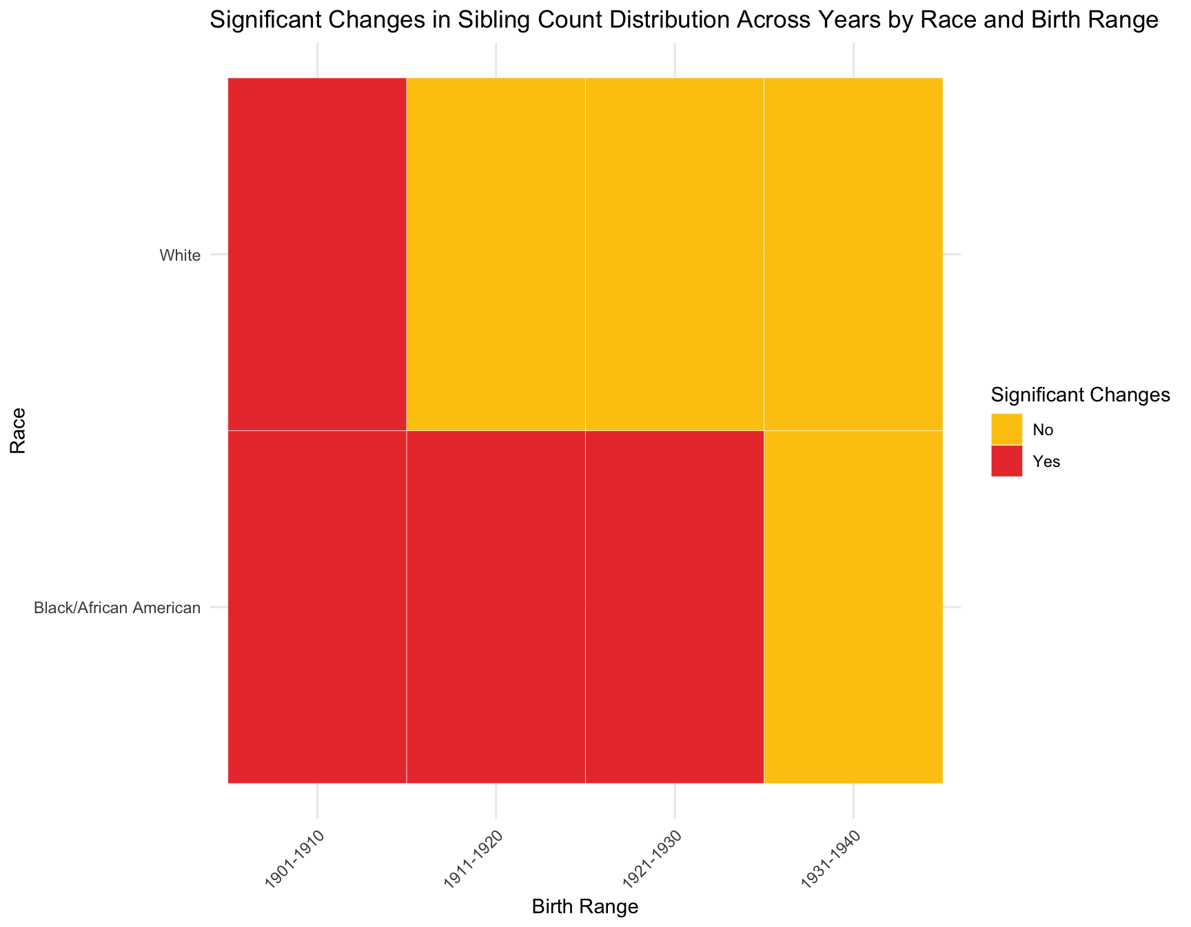
- Interpret results:
- Identify which cohorts show stable sibling distributions.
- Compare stability patterns to those observed in the children distribution analysis.
- Discuss implications of stability or lack thereof for understanding family structure changes over time.
Apply similar analysis performed in the children’s part:
- Zero Inflation: Check if the proportion of individuals with zero siblings changes significantly over time for the same cohort.
best_models_sib <- best_models_sib %>%
  mutate(Cohort = mapply(calculate_cohort, Census_Year, AGE_RANGE)) %>%
  dplyr::select(Race, Census_Year, AGE_RANGE, Best_Model, Cohort)

df_merg2 <- df2 %>%
  rename(Census_Year = YEAR, Race = RACE)

# Perform a left join to merge the data frames
merged_data_sib <- left_join(df_merg2, best_models_sib, by = c("Race", "Census_Year", "AGE_RANGE"))
## divided the corhort by race
merged_df_black2 <- merged_data_sib %>% filter(Race == "Black/African American")
merged_df_white2 <- merged_data_sib %>% filter(Race == "White")# Filter cohorts with more than one census year
cohort_counts <- merged_df_black2 %>%
group_by(Cohort) %>%
summarise(Unique_Census_Years = n_distinct(Census_Year)) %>%
filter(Unique_Census_Years > 1)
# Get the list of cohorts for testing
cohorts_for_test <- cohort_counts$Cohort
# Initialize results data frame
results_black2 <- data.frame(RACE = character(), Cohort = character(), Chi_Square = numeric(), p_value = numeric(), stringsAsFactors = FALSE)
# Loop through each cohort and run the chi-square test
for (cohort in cohorts_for_test) {
cohort_data <- merged_df_black2 %>% filter(Cohort == cohort)
# Create contingency table
contingency_table <- table(cohort_data$Census_Year, cohort_data$n_siblings == "0")
# Perform the chi-square test only if more than one row is in the table
if (nrow(contingency_table) > 1) {
test_result <- chisq.test(contingency_table)
# Append results to the results data frame
results_black2 <- rbind(results_black2, data.frame(
RACE = "Black/African American",
Cohort = cohort,
Chi_Square = test_result$statistic,
p_value = test_result$p.value
))
}
}
results_black2 <- results_black2 %>%
mutate(Significance = ifelse(p_value > 0.05, "No", "Yes"))
print(results_black2) RACE Cohort Chi_Square p_value Significance
X-squared Black/African American 1901-1910 2.7595148 0.09667755 No
X-squared1 Black/African American 1911-1920 3.1588986 0.20608856 No
X-squared2 Black/African American 1921-1930 6.4474388 0.03980673 Yes
X-squared3 Black/African American 1931-1940 0.8166152 0.36617166 No# Filter cohorts with more than one census year
cohort_counts <- merged_df_white2 %>%
group_by(Cohort) %>%
summarise(Unique_Census_Years = n_distinct(Census_Year)) %>%
filter(Unique_Census_Years > 1)
# Get the list of cohorts for testing
cohorts_for_test <- cohort_counts$Cohort
# Initialize results data frame
results_white2 <- data.frame(RACE = character(), Cohort = character(), Chi_Square = numeric(), p_value = numeric(), stringsAsFactors = FALSE)
# Loop through each cohort and run the chi-square test
for (cohort in cohorts_for_test) {
cohort_data <- merged_df_white2 %>% filter(Cohort == cohort)
# Create contingency table
contingency_table <- table(cohort_data$Census_Year, cohort_data$n_siblings == "0")
# Perform the chi-square test only if more than one row is in the table
if (nrow(contingency_table) > 1) {
test_result <- chisq.test(contingency_table)
# Append results to the results data frame
results_white2 <- rbind(results_white2, data.frame(
RACE = "White",
Cohort = cohort,
Chi_Square = test_result$statistic,
p_value = test_result$p.value
))
}
}
results_white2 <- results_white2 %>%
mutate(Significance = ifelse(p_value > 0.05, "No", "Yes"))
print(results_white2) RACE Cohort Chi_Square p_value Significance
X-squared White 1901-1910 46.930953 7.353216e-12 Yes
X-squared1 White 1911-1920 120.015145 8.690450e-27 Yes
X-squared2 White 1921-1930 79.061388 6.792628e-18 Yes
X-squared3 White 1931-1940 2.776021 9.568561e-02 No- Family Size: Test if the mean or variance in the number of siblings changes for the same cohort over time.
sum_table_sib <- merged_data_sib %>% group_by(Race, Cohort, Census_Year) %>%
  summarise(
    Mean = mean(chborn_num),
    Variance = var(chborn_num))
`summarise()` has grouped output by 'Race', 'Cohort'. You can override using
the `.groups` argument.merged_sib <- left_join(merged_data_sib, sum_table_sib, by = c("Race","Cohort","Census_Year")) %>% dplyr::select(Race, Cohort, Census_Year, Mean, Variance)
sum_table_black = merged_sib %>% filter(Race == "Black/African American")
sum_table_white = merged_sib %>% filter(Race == "White")##Test for Black population
cohorts1 <- unique(sum_table_black$Cohort)
# Loop through each cohort and apply ANOVA for Mean and Variance
for (cohort in cohorts1) {
# Filter data for the specific cohort
cohort_data_b <- sum_table_black[sum_table_black$Cohort == cohort, ]
# Check if there are at least two unique Census_Year values
if (length(unique(cohort_data_b$Census_Year)) < 2) {
cat("\nCohort:", cohort, "has only one Census Year. Skipping ANOVA.\n")
next
}
# Perform ANOVA for Mean
anova_mean_result <- aov(Mean ~ factor(Census_Year), data = cohort_data_b)
# Perform ANOVA for Variance
anova_variance_result <- aov(Variance ~ factor(Census_Year), data = cohort_data_b)
# Output the results
cat("\nCohort:", cohort)
cat("\nANOVA for Mean Family Size:\n")
print(summary(anova_mean_result))
cat("\nANOVA for Variance in Family Size:\n")
print(summary(anova_variance_result))
}
Cohort: 1891-1900 has only one Census Year. Skipping ANOVA.

Cohort: 1911-1920
ANOVA for Mean Family Size:
                       Df Sum Sq Mean Sq   F value Pr(>F)
factor(Census_Year)     2  5.453   2.727 8.507e+23 <2e-16 ***
Residuals           38001  0.000   0.000
---
Signif. codes:  0 '***' 0.001 '**' 0.01 '*' 0.05 '.' 0.1 ' ' 1

ANOVA for Variance in Family Size:
                       Df Sum Sq Mean Sq   F value Pr(>F)
factor(Census_Year)     2   1099   549.7 7.821e+25 <2e-16 ***
Residuals           38001      0     0.0
---
Signif. codes:  0 '***' 0.001 '**' 0.01 '*' 0.05 '.' 0.1 ' ' 1

Cohort: 1901-1910
ANOVA for Mean Family Size:
                       Df Sum Sq Mean Sq   F value Pr(>F)
factor(Census_Year)     1  77.51   77.51 7.094e+25 <2e-16 ***
Residuals           22789   0.00    0.00
---
Signif. codes:  0 '***' 0.001 '**' 0.01 '*' 0.05 '.' 0.1 ' ' 1

ANOVA for Variance in Family Size:
                       Df Sum Sq Mean Sq   F value Pr(>F)
factor(Census_Year)     1   2547    2547 8.424e+26 <2e-16 ***
Residuals           22789      0       0
---
Signif. codes:  0 '***' 0.001 '**' 0.01 '*' 0.05 '.' 0.1 ' ' 1

Cohort: -Inf-1890 has only one Census Year. Skipping ANOVA.

Cohort: 1921-1930
ANOVA for Mean Family Size:
                       Df Sum Sq Mean Sq   F value Pr(>F)
factor(Census_Year)     2    417   208.5 4.477e+26 <2e-16 ***
Residuals           43042      0     0.0
---
Signif. codes:  0 '***' 0.001 '**' 0.01 '*' 0.05 '.' 0.1 ' ' 1

ANOVA for Variance in Family Size:
                       Df Sum Sq Mean Sq   F value Pr(>F)
factor(Census_Year)     2   3122    1561 4.647e+25 <2e-16 ***
Residuals           43042      0       0
---
Signif. codes:  0 '***' 0.001 '**' 0.01 '*' 0.05 '.' 0.1 ' ' 1

Cohort: -Inf-1900 has only one Census Year. Skipping ANOVA.

Cohort: 1931-1940
ANOVA for Mean Family Size:
                       Df  Sum Sq Mean Sq   F value Pr(>F)
factor(Census_Year)     1 0.03475 0.03475 1.223e+22 <2e-16 ***
Residuals           22555 0.00000 0.00000
---
Signif. codes:  0 '***' 0.001 '**' 0.01 '*' 0.05 '.' 0.1 ' ' 1

ANOVA for Variance in Family Size:
                       Df Sum Sq Mean Sq  F value Pr(>F)
factor(Census_Year)     1  301.2   301.2 6.73e+25 <2e-16 ***
Residuals           22555    0.0     0.0
---
Signif. codes:  0 '***' 0.001 '**' 0.01 '*' 0.05 '.' 0.1 ' ' 1

Cohort: -Inf-1910 has only one Census Year. Skipping ANOVA.

Cohort: 1941-1950 has only one Census Year. Skipping ANOVA.

Cohort: -Inf-1920 has only one Census Year. Skipping ANOVA.
##Test for White population
cohorts2 <- unique(sum_table_white$Cohort)
# Loop through each cohort and apply ANOVA for Mean and Variance
for (cohort in cohorts2) {
# Filter data for the specific cohort
cohort_data_w <- sum_table_white[sum_table_white$Cohort == cohort, ]
# Check if there are at least two unique Census_Year values
if (length(unique(cohort_data_w$Census_Year)) < 2) {
cat("\nCohort:", cohort, "has only one Census Year. Skipping ANOVA.\n")
next
}
# Perform ANOVA for Mean
anova_mean_result <- aov(Mean ~ factor(Census_Year), data = cohort_data_w)
# Perform ANOVA for Variance
anova_variance_result <- aov(Variance ~ factor(Census_Year), data = cohort_data_w)
# Output the results
cat("\nCohort:", cohort)
cat("\nANOVA for Mean Family Size:\n")
print(summary(anova_mean_result))
cat("\nANOVA for Variance in Family Size:\n")
print(summary(anova_variance_result))
}
Cohort: 1891-1900 has only one Census Year. Skipping ANOVA.

Cohort: 1911-1920
ANOVA for Mean Family Size:
                        Df Sum Sq Mean Sq   F value Pr(>F)
factor(Census_Year)      2  535.2   267.6 4.546e+24 <2e-16 ***
Residuals           365210    0.0     0.0
---
Signif. codes:  0 '***' 0.001 '**' 0.01 '*' 0.05 '.' 0.1 ' ' 1

ANOVA for Variance in Family Size:
                        Df Sum Sq Mean Sq   F value Pr(>F)
factor(Census_Year)      2   1563   781.4 4.723e+25 <2e-16 ***
Residuals           365210      0     0.0
---
Signif. codes:  0 '***' 0.001 '**' 0.01 '*' 0.05 '.' 0.1 ' ' 1

Cohort: 1901-1910
ANOVA for Mean Family Size:
                        Df Sum Sq Mean Sq   F value Pr(>F)
factor(Census_Year)      1   1281    1281 9.604e+25 <2e-16 ***
Residuals           226142      0       0
---
Signif. codes:  0 '***' 0.001 '**' 0.01 '*' 0.05 '.' 0.1 ' ' 1

ANOVA for Variance in Family Size:
                        Df Sum Sq Mean Sq   F value Pr(>F)
factor(Census_Year)      1  352.5   352.5 6.248e+23 <2e-16 ***
Residuals           226142    0.0     0.0
---
Signif. codes:  0 '***' 0.001 '**' 0.01 '*' 0.05 '.' 0.1 ' ' 1

Cohort: -Inf-1890 has only one Census Year. Skipping ANOVA.

Cohort: -Inf-1900 has only one Census Year. Skipping ANOVA.

Cohort: 1921-1930
ANOVA for Mean Family Size:
                        Df Sum Sq Mean Sq   F value Pr(>F)
factor(Census_Year)      2  653.9     327 8.029e+23 <2e-16 ***
Residuals           394507    0.0       0
---
Signif. codes:  0 '***' 0.001 '**' 0.01 '*' 0.05 '.' 0.1 ' ' 1

ANOVA for Variance in Family Size:
                        Df Sum Sq Mean Sq   F value Pr(>F)
factor(Census_Year)      2    224     112 2.455e+24 <2e-16 ***
Residuals           394507      0       0
---
Signif. codes:  0 '***' 0.001 '**' 0.01 '*' 0.05 '.' 0.1 ' ' 1

Cohort: 1931-1940
ANOVA for Mean Family Size:
                        Df Sum Sq Mean Sq   F value Pr(>F)
factor(Census_Year)      1  1.829   1.829 8.533e+22 <2e-16 ***
Residuals           179944  0.000   0.000
---
Signif. codes:  0 '***' 0.001 '**' 0.01 '*' 0.05 '.' 0.1 ' ' 1

ANOVA for Variance in Family Size:
                        Df Sum Sq Mean Sq   F value Pr(>F)
factor(Census_Year)      1  79.94   79.94 1.017e+24 <2e-16 ***
Residuals           179944   0.00    0.00
---
Signif. codes:  0 '***' 0.001 '**' 0.01 '*' 0.05 '.' 0.1 ' ' 1

Cohort: -Inf-1910 has only one Census Year. Skipping ANOVA.

Cohort: -Inf-1920 has only one Census Year. Skipping ANOVA.

Cohort: 1941-1950 has only one Census Year. Skipping ANOVA.- Model Fit: Analyze if the best-fitting model for the cohort changes over time.
ggplot(best_models_sib, aes(x = Census_Year, y = Cohort, fill = Best_Model)) +
  geom_tile(color = "white", lwd = 0.5, linetype = 1) + # Create the tiles
  facet_wrap(~Race, nrow = 2) + # Facet by Race
  scale_fill_manual(values = c("Poisson" = "#0072B2", "Zero_Inflated_NB" = "#F0E442", "Negative_Binomial" = "grey")) +
  labs(
    title = "Best Model(siblings) by Race, Census Year, and Cohort(Birth Range)",
    x = "Census Year",
    y = "Birth Range",
    fill = "Best Model"
  ) +
  theme_minimal() +
  theme(
    plot.title = element_text(size = 14, face = "bold"),
    legend.position = "bottom"
  )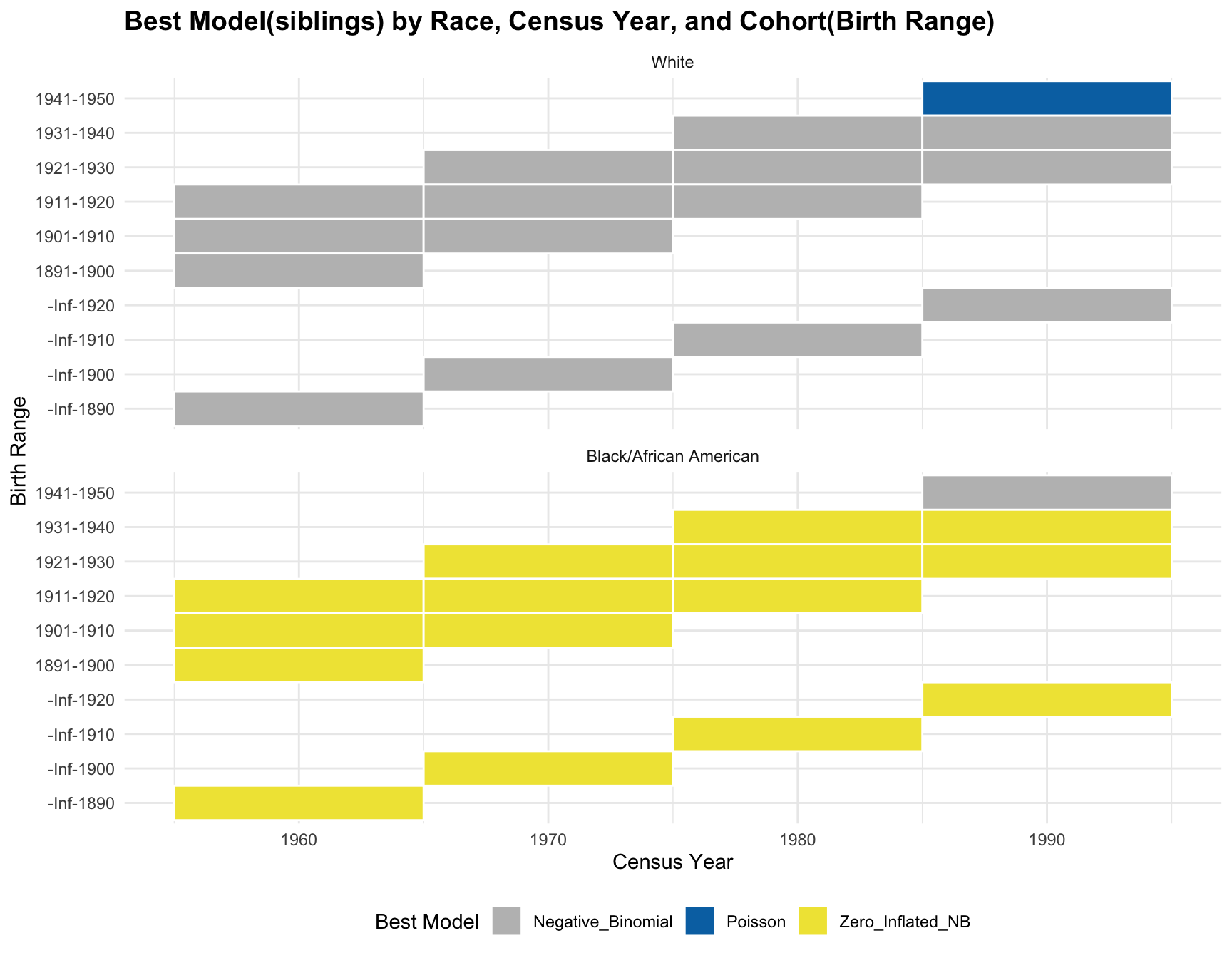
[Instructions for Manqing] Plot Across Census Years Siblings
Objective
Create a visualization showing how sibling distributions change across census years for different races and birth ranges.
Steps
Use the sibling distribution data (
df_sibling_proportions).Create a multi-panel plot:
- X-axis: Number of siblings (0 to 12+)
- Y-axis: Proportion
- Color: Census Year
- Facet by: RACE and AGE_RANGE
Use
ggplot2to create the plot:
df_sibling_proportions %>%
  filter(n_siblings >= 0, sibling_count >= 0, proportion >= 0) %>% ggplot(aes(x = n_siblings, y = proportion, color = factor(YEAR))) +
 geom_line() +
 facet_grid(RACE ~ AGE_RANGE) +
 labs(title = "Sibling Distribution Across Census Years",
      x = "Number of Siblings", y = "Proportion", color = "Census Year") +
 theme_minimal() +
 theme(axis.text.x = element_text(hjust = 1))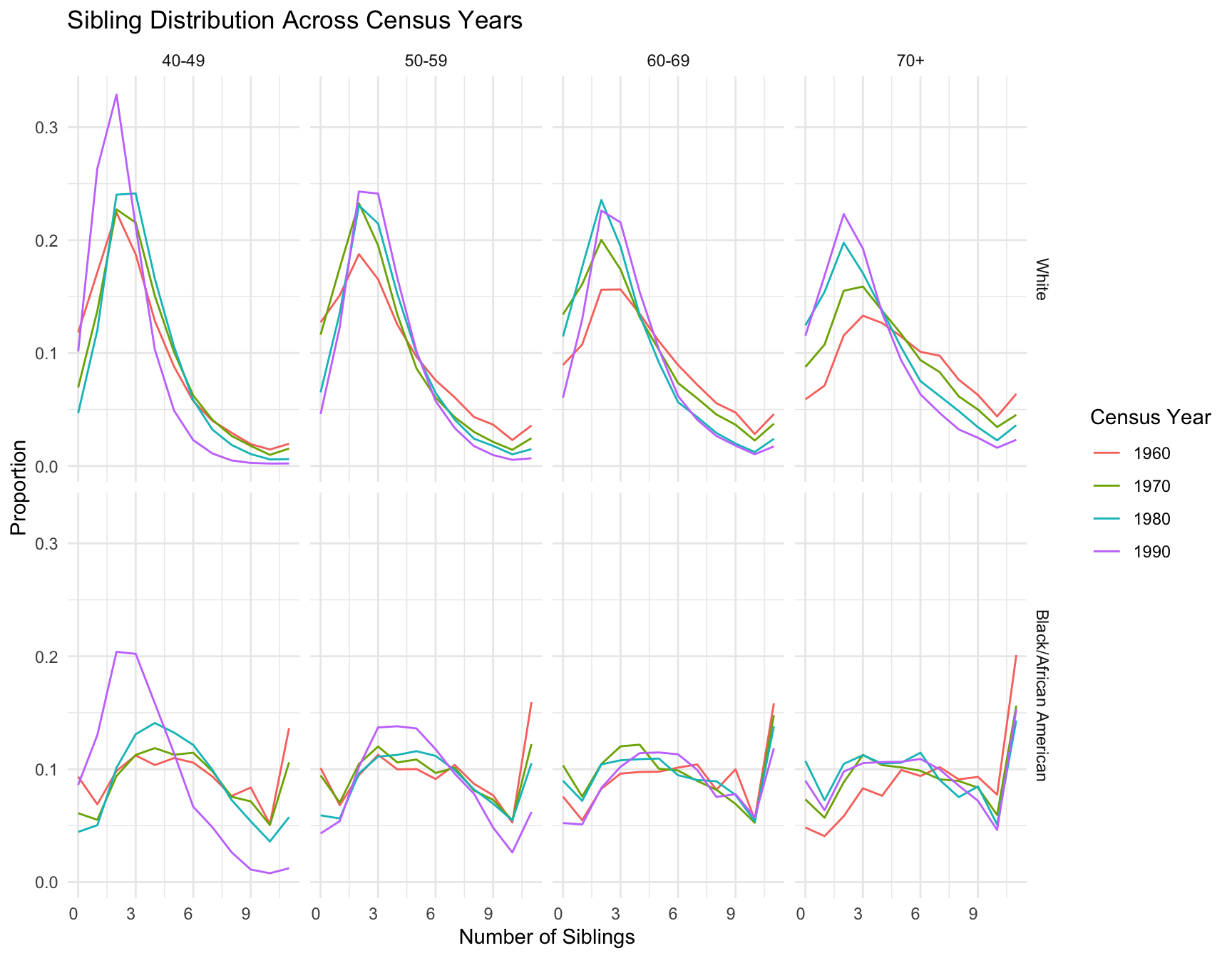
- Analyze the plot:
- Identify trends in sibling distribution changes over time.
- Compare patterns between races and across birth ranges.
- Note any significant shifts or stable periods.
- Compare with children distribution plot:
- Highlight similarities and differences in trends.
- Discuss what these comparisons reveal about changing family structures.
Remember to reference your findings from the children distribution analysis when discussing the results, highlighting any notable similarities or differences between the two analyses.
sessionInfo()